[

Magnetooptical sum rules close to the Mott transition

Abstract

We derive new sum rules for the real and imaginary parts of the frequency-dependent Hall constant and Hall conductivity. As an example, we discuss their relevance to the doped Mott insulator that we describe within the dynamical mean-field theory of strongly correlated electron systems.

]

The ac Hall effect can provide valuable insights into the dynamics of an electronic medium. This has recently been demonstrated in the case of high-$T_{c}$ superconductors [1, 2]: Various theoretical models based on different scattering mechanisms agree that the anomalous frequency and temperature dependences of the Hall effect are closely intertwined, but they differ in their predictions about these dependences [3]. So far, experiments cannot discriminate between these models, but they will possibly be able to do so in the future [3].

The magnetooptical response of charge carriers can be probed by the frequency-dependent Hall conductivity, Hall constant, or Hall angle. Recently, a sum rule for the Hall angle has been derived [4] that is similar to the well-known $f$-sum rule for the optical conductivity [5]. In this paper, we derive new sum rules for the real and imaginary parts of the two other magnetotransport probes. Such sum rules are useful: First, they help elucidating how the corresponding spectral weight is redistributed upon changing the temperature or the doping level. Second, they provide exact constraints on the interdependence of Hall effect-related quantities and thus help interpreting experimental data. For example, the sum rules for the ac Hall constant relate its low-frequency behavior to its infinite-frequency limit. This can be useful because experimentally, only the microwave domain and the far infrared are attainable sufficiently reliably [2, 3], whereas the calculation of the Hall constant simplifies considerably in the high-frequency limit [6].

We shall first derive the sum rules for the Hall conductivity and Hall constant quite generally. Then, to illustrate their application, we shall discuss some aspects of the magnetooptical response of correlated electrons close to the density-driven Mott transition.

We start by considering the ac conductivities. In terms of the dissipative part of the current-current correlation function,

$$\chi_{\nu\mu}^{\prime\prime}(\omega)=\int_{-\infty}^{\infty}dt\,{1\over 2}\langle[\hat{J}_{\nu}(t),\hat{J}_{\mu}(0)]\rangle e^{i\omega t},$$ (1)

the conductivity tensor reads

$$\sigma_{\nu\mu}(\omega)=ie^{2}{\cal P}\int_{-\infty}^{\infty}{d\tilde{\omega}\over\pi}\frac{\chi_{\nu\mu}^{\prime\prime}(\tilde{\omega})}{\tilde{\omega}(\omega-\tilde{\omega})}+e^{2}\frac{\chi_{\nu\mu}^{\prime\prime}(\omega)}{\omega}.$$ (2)

Here, ${\cal P}$ indicates principal-value integration. From time reversal invariance, homogeneity of time, and the Hermiticity of the current operators, we may deduce the following symmetry properties [7]:

$$\chi_{xx}^{\prime\prime}(\omega) =$$ odd & real (3)

$$\chi_{xy}^{\prime\prime}(\omega) = \mbox{even \& wholly imaginary},$$ (4)

where Eq. (4) holds to first order in the magnetic field. Eqs. (3) and (4) imply that the real parts of $\sigma_{xx}(\omega)$ and $\sigma_{xy}(\omega)$ are even while their imaginary ones are odd. We also see that the dc Hall conductivity is finite only if

$$\chi_{xy}^{\prime\prime}(0)=0,$$ (5)

and derive the first couple of sum rules:

$$\int_{0}^{\infty}d\omega\,\Re\sigma_{xy}(\omega) = 0,$$ (6)

$$\int_{-\infty}^{\infty}d\omega\,\frac{\omega\Im\sigma_{xy}(\omega)}{\pi e^{2}} = -i\langle[\hat{J}_{x},\hat{J}_{y}]\rangle.$$ (7)

To prove Eq. (6), we close the path of integration along a semicircle at infinity in the upper-half complex-frequency ($z$) plane and apply Cauchy’s theorem. The integral on the semicircle does not contribute since the leading high-frequency behavior of $\sigma_{xy}(z)$ is $1/z^{2}$. The sum rule (7) is similar to the $f$-sum rule of the optical conductivity,

$$\int_{-\infty}^{\infty}d\omega\,\frac{\Re\sigma_{xx}(\omega)}{\pi e^{2}}=i\langle[\hat{J}_{x},\hat{P}_{x}]\rangle=\chi^{0},$$ (8)

where $\hat{P}_{x}$ is the polarization operator satisfying $\hat{J}_{x}(t)=\partial\hat{P}_{x}(t)/\partial t$, and $\chi^{0}=\int d\omega\,\chi_{xx}^{\prime\prime}(\omega)/\pi\omega$ is the static current-current correlation function, which is positive definite. To interprete the right-hand sides of Eqs. (7) and (8), we first note that the Hall frequency $\omega_{H}\equiv-i\langle[\hat{J}_{x},\hat{J}_{y}]\rangle/\chi^{0}$ is the generalization of the cyclotron frequency to the lattice [7, 4]. Its sign determines that of the infinite-frequency Hall constant,

$$R_{H}^{*}=\lim_{H\rightarrow 0}\frac{N\omega_{H}}{e^{2}\chi^{0}H},$$ (9)

which was considered by Shastry et al. [6]. Here, $N$ denotes the total number of lattice sites. Second, the Drude-theory expression $\sigma_{xx}(\omega)=\frac{\omega_{p}^{2}/4\pi}{1/\tau-i\omega}$ yields $\chi^{0}=\omega_{p}^{2}/4\pi e^{2}$, where $e$ is the charge of an electron and $\omega_{p}$ the plasma frequency. In general, however, $\chi^{0}$ and $\omega_{H}$ depend on all external and model parameters such as temperature, band filling, and correlation strength.

Before proceeding, we compare the sum rules (7) and (8). In both cases, the contribution of a band $\epsilon(\vec{k})$ to the right-hand side can be represented as a weighted average of the momentum-distribution function, $n_{\vec{k}\sigma}$, over the Brillouin zone (BZ), where the weight function is determined by the inverse mass tensor [6]: $-i\langle[\hat{J}_{x},\hat{J}_{y}]\rangle=He\sum_{\vec{k}\sigma}\det(\epsilon^{\nu\mu}_{\vec{k}})n_{\vec{k}\sigma}$ and $\chi^{0}=\sum_{\vec{k}\sigma}\epsilon^{xx}_{\vec{k}}n_{\vec{k}\sigma}$. Here, upper indices indicate differentiation with respect to a component of the Bloch vector, such as in, say, $\epsilon_{\vec{k}}^{x}={\partial\epsilon_{\vec{k}}/\partial k_{x}}$. $H$ is the magnetic field and is assumed to point in the $z$ direction, and $\nu,\mu=x,y$. In many semiconductors, only Bloch states close to the minima of the conduction band or the maxima of the valence band contribute. Then, one can replace the inverse mass tensor by its value at the respective band edge. Thus, the sum rules (7) and (8) are seen to relate hard-to-obtain experimental information to, first, the number of carriers and, second, to the mass tensor at a band edge which can be measured in a cyclotron-resonance experiment. In a strongly correlated system, on the other hand, the momentum-distribution function receives contributions from the entire BZ, and the above-mentioned BZ averages may no longer be easy to determine experimentally [6].

Next, we investigate the ac Hall constant. In Ref. [7], it has been decomposed into its infinite-frequency limit (9) and a memory-function contribution which can be represented in terms of a spectral function $k(\omega)$:

$$R_{H}(\omega)=R_{H}^{*}\left(1+\int_{-\infty}^{\infty}d\tilde{\omega}\,{\cal P}\frac{k(\tilde{\omega})\tilde{\omega}}{\tilde{\omega}-\omega}\right)+i\pi R_{H}^{*}k(\omega)\omega.$$ (10)

$k(\omega)$ was shown to be even and real. Therefore, the real and imaginary parts of $R_{H}(\omega)$ are even and odd, respectively. We also establish nontrivial sum rules for the ac Hall constant:

$$\int_{0}^{\infty}d\omega\,\left[\Re R_{H}(\omega)-R_{H}^{*}\right]=0,$$ (11)

$$\int_{-\infty}^{\infty}\frac{d\omega}{\pi}\,\frac{\Im R_{H}(\omega)}{\omega}=R_{H}-R_{H}^{*},$$ (12)

where $R_{H}$ is the dc Hall constant. Eq. (11) holds because the leading high-frequency behavior of $R_{H}(z)-R_{H}^{*}$ is $1/z^{2}$ [7]. Eq. (12) is a Kramers-Kronig relation. The sum rules (11) and (12) are interesting because they relate the Hall constant at low frequencies to its infinite-frequency limit. The low-frequency regime is attainable in experiments [2], whereas the high-frequency limit is much easier to handle theoretically. The sum rule (11) implies that $R_{H}$ cannot go over from its dc value to its infinite-frequency limit monotonically.

Finally, we quote a sum rule for the Hall angle $t_{H}(\omega)\equiv\tan\theta_{H}(\omega)=\sigma_{xy}(\omega)/\sigma_{xx}(\omega)$ that was derived in Ref. [4]:

$$\int_{-\infty}^{\infty}\frac{d\omega}{\pi}\,\Re t_{H}(\omega)=\omega_{H}.$$ (13)

By contrast to the $f$-sum rule in Eq. (8), none of our sum rules involves a positive definite integrand. As a consequence, we expect our sum rules to become fully useful only in conjunction with some theoretical understanding of the problem involved.

We now apply the above-mentioned sum rules to the doped Mott insulator, which we describe by the single-band Hubbard model with bare bandwidth $2D$ and on-site repulsion $U$. We are primarily interested in the physics close to half filling, $\delta\equiv 1-n\ll 1$, where $n$ denotes the average occupancy per lattice site. In the limit of infinite spatial dimensions, all vertex corrections of the conductivity tensor vanish which implies [8]

$$\sigma_{xx}(i\omega_{m}) = {2ie^{2}\over N\beta}\sum_{\vec{k}n}(\epsilon_{\vec{k}}^{x})^{2}G_{\vec{k}|n}\,\frac{G_{\vec{k}|n+m}-G_{\vec{k}|n}}{i\omega_{m}},$$ (14)

$$\sigma_{xy}(i\omega_{m}) = {e^{3}H\over N\beta}\sum_{\vec{k}n}\left|\begin{array}[]{cc}\epsilon_{\vec{k}}^{x}\epsilon_{\vec{k}}^{x}&\epsilon_{\vec{k}}^{xy}\\[6.02773pt] \epsilon_{\vec{k}}^{y}\epsilon_{\vec{k}}^{x}&\epsilon_{\vec{k}}^{yy}\end{array}\right|G_{\vec{k}|n}^{2}\,\frac{G_{\vec{k}|n+m}-G_{\vec{k}|n-m}}{i\omega_{m}}.$$ (17)

In each equation, a spin factor 2 has been taken into account and $\beta=1/T$ is the inverse temperature. $i\omega_{n}$ and $i\omega_{m}$ are fermionic and bosonic Matsubara frequencies, respectively. The single-particle Green’s function is given by $G_{\vec{k}|n}^{-1}=i\omega_{n}+\mu-\epsilon_{\vec{k}}-\Sigma(i\omega_{n})$, where the local self-energy $\Sigma(i\omega_{n})$ must be calculated by solving a single-impurity Anderson model supplemented by a self-consistency condition [9]. Earlier work on the Hall effect in infinite dimensions was carried out in Refs. [10, 11, 12]. We compute the ac conductivities (14) and (17) numerically by using the tight-binding band $\epsilon_{\vec{k}}=-(D/\sqrt{2d})\sum_{j}\cos(k_{j}a)$ in $d$ dimensions, where $a$ is the lattice spacing. We use the iterated perturbation theory (IPT), which can be shown to obey our sum rules exactly.

Our main focus is on the frequency regime well below the Mott-Hubbard gap $U$. The relevant part of the single-particle spectrum then consists of two distinct features: an incoherent lower Hubbard band (LHB) and, provided the temperature is low enough, a quasiparticle resonance (QPR) at the Fermi level. As the doping level is increased, the QPR merges with the LHB from above.

Accordingly, there are two widely different energy scales close to the Mott transition: a coherence temperature $T_{\mbox{coh}}$ below which Fermi-liquid properties begin to be observed, and $D$ which sets the scale for incoherent excitations. The width of the QPR defines a second low-energy scale $T^{*}$. The ac conductivities (14) and (17) reflect the possible transitions within the single-particle spectrum. For $T<T_{\mbox{coh}}$, this means that the integrands of all sum rules roughly decompose into two features: First, a narrow one at zero frequency which is due to transitions within the QPR. Consequently, its width scales at most with $T^{*}$. We shall see below that this feature can be resolved in the Fermi-liquid regime so its width does not exceed the smaller scale $T_{\mbox{coh}}$. Second, a feature around a frequency $\omega_{1}$ that measures the distance between the maxima of the LHB and the QPR, $\omega_{1}\sim D$. At high temperatures, on the other hand, the integrands are solely determined by transitions from occupied to unoccupied states within the LHB, and $D$ is the only energy scale.

In the Fermi-liquid regime, $T,\omega<T_{\mbox{coh}}$, the conductivities can be cast into the Drude forms $\sigma_{xx}(\omega)=\frac{\omega_{p}^{*2}/4\pi}{1/\tau^{*}-i\omega}$ and $\sigma_{xy}(\omega)=\frac{\omega_{c}^{*}\omega_{p}^{*2}/4\pi}{(1/\tau^{*}-i\omega)^{2}}$ with renormalized parameters. Here, the renormalized plasma frequency behaves as $\omega_{p}^{*2}\sim D\delta$ [13]; $1/\tau^{*}\sim\delta\,\mbox{Im}\Sigma_{R}(\omega=0,T)$, where $\Sigma_{R}$ is the retarded self-energy in the absence of disorder; $\omega_{c}^{*}\sim\omega_{c}\delta$ where $\omega_{c}$ is the cyclotron frequency of noninteracting electrons on the same lattice. The renormalized plasma and cyclotron frequencies must not be confused with the bare ones defined by the sum rules (8) and (13), respectively.

Expanding Eqs. (14) and (17) to leading order in $1/T$ as explained in Ref. [12] shows that both conductivities are suppressed by a factor $\delta$ close to the Mott transition. Approximate expressions for the dissipative parts of the conductivities, which capture the doping and temperature dependences in the region $T,\omega>T^{*}$, $\omega\ll 2D$, are given by $\Re\sigma_{xx}(\omega)\sim e^{2}\delta\,\frac{1-\exp(-|\omega|/T)}{|\omega|}$ and $\Im\sigma_{xy}(\omega)\sim e^{3}H\delta\,\mbox{sgn}(\omega)[1-\exp(-|\omega|/T)]/D$. The last relation only holds for a generic band that does not have the bipartite-lattice property discussed in Ref. [12].

We now discuss the qualitative forms of the functions governing the sum rules (6), (7), (11), (12), and (13) more specifically. In all plots, we have chosen $\delta=0.1$ and $U=4$.

Real part of the Hall conductivity.–Its high-frequency behavior is given by $\sigma_{xy}(\omega)\simeq-e^{2}\chi^{0}\omega_{H}/\omega^{2}$ and therefore has the opposite sign as $R_{H}^{*}$ in Eq. (9). On the other hand, its dc value has the same sign as $R_{H}$. Close to half filling, and for intermediate temperatures and up, $R_{H}$ and $R_{H}^{*}$ have the same sign [11]. Since in this parameter regime, the only energy scale is $D$, $\Re\sigma_{xy}(\omega)$ changes its sign once at a scale of order $D$ to satisfy sum rule (6). For $T<T_{\mbox{coh}}$, $R_{H}^{*}$ remains hole-like while $R_{H}$ becomes electron-like [11]. Then, the sum rule (6) requires at least one further sign change at a scale $\omega\sim T_{\mbox{coh}}$. This prediction is corroborated by our numerical investigation, Fig. 1 displays the frequency-dependent Hall conductivity for $T=0.015D$.

Imaginary part of the Hall conductivity.–Fig. 2 displays the integrand of the sum rule (7), which is proportional to the spectral function (4). We have normalized this function to 1 to facilitate the comparison between curves belonging to different temperatures. For $T>T^{*}$, this function hardly depends on temperature. Its “M-shaped” form is consistent with Eq. (5) and the fact that $D$ is the only energy scale. As the temperature is decreased to below $T^{*}$, the spectral weight is redistributed to comply with the emergence of two energy scales $T_{\mbox{coh}}$ and $\omega_{1}$, the Drude form in the Fermi-liquid regime, and the fact that the overall weight is positive.

Hall angle.–The real part of the Hall angle defined before Eq. (13) closely resembles that of the previously considered function, except that it is not subject to a condition like Eq. (5).

Hall constant.–Close to half filling and for $T>T^{*}$, $R_{H}$ is greater than $R_{H}^{*}$ [11]. Then, $\Re R_{H}(\omega)$ satisfies the sum rule (11) as follows: Starting from its dc value, $\Re R_{H}(\omega)$ first decreases monotonically as a function of frequency, drops to below its infinite-frequency level at a frequency of order $D$, and finally rises to approach $R_{H}^{*}$ from below. In the opposite limit of very low temperatures, we show a curve for $T=0.015D$ in the main panel of Fig. 3, along with a better resolution of its low-frequency part in the left inset. $R_{H}^{*}$ (dotted line) is seen to be positive, while $R_{H}<0$ (not discernible), in agreement with Ref. [11]. In addition, $R_{H}(\omega)$ hardly depends on frequency in the Fermi-liquid regime, as expected from the Drude parametrizations of $\sigma_{xx}(\omega)$ and $\sigma_{xy}(\omega)$. To counterbalance the drop of the dc value to below $R_{H}^{*}$, a peak-like structure has piled up to above the $R_{H}^{*}$ level at the other energy scale, $\omega\sim D$ . The structure about $\omega\sim 3D$ arises from the upper Hubbard band. At very high frequencies, $\Re R_{H}(\omega)$ approaches its asymptotic value according to a $1/\omega^{2}$ law. In the right inset of Fig. 3, we display a curve at the cross-over temperature $T=0.15D$. Like in the high-temperature regime, $R_{H}>R_{H}^{*}>0$. But the sign change of $\Re R_{H}(\omega)-R_{H}^{*}$ is already shifted to higher frequencies, signalling the emergence of the peak at $\omega\sim D$ as the temperature is lowered.

Finally, Fig. 4 displays the function $k(\omega)$, which is proportional to the integrand of the sum rule (12) and which has not been normalized to 1. As the temperature is decreased from well above (not shown in Fig. 4) to well below $T^{*}$, a single peak of width $D$ decomposes into a narrow one at $\omega=0$ and of width smaller than $T_{\mbox{coh}}$, and a feature around $\omega\sim\omega_{1}$ which involves a sign change. In the normal state of cuprates such as La_2-xSr_xCuO₄, $k(\omega)$ is resonance-like and has a width given by the anomalous relaxation rate $1/\tau_{H}$ which exhibits a $T^{2}$ law [7]. Instead, we find a width of order $D$ for temperatures above $T^{*}$ where $R_{H}>0$. Similarly, the dynamical mean-field theory predicts that Kohler’s rule is replaced by $\Delta\rho/\rho\sim(\omega_{c}/D)^{2}$ in the high-temperature regime [12], whereas experiments on cuprates are consistent with $\Delta\rho/\rho\sim(\omega_{c}\tau_{H})^{2}$ as suggested by Terasaki et al. [14]. Here, $\Delta\rho$ is the magnetoresistance.

In summary, we have derived sum rules for the real and imaginary parts of the Hall conductivity and Hall constant. We have applied them, along with another one for the Hall angle, to the doped Mott insulator.

This work was supported by NSF DMR 95-29138. E.L. is funded by the Deutsche Forschungsgemeinschaft.

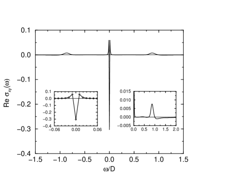
FIG. 1.: Real part of the Hall conductivity for $T=0.015D$. The insets magnify the structures at $\omega=0$ (left one) and $\omega=D$ (right one).

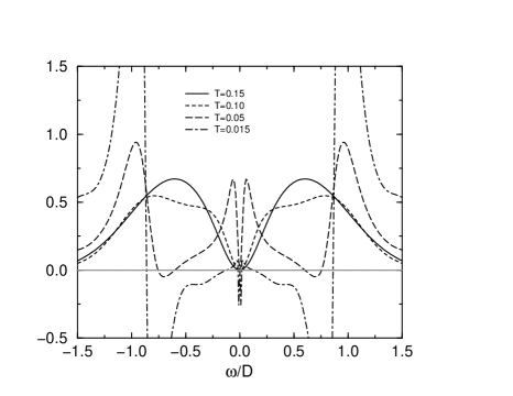
FIG. 2.: $\chi_{xy}^{\prime\prime}(\omega)$ normalized to 1.

FIG. 3.: $\Re R_{H}(\omega)$ (solid lines) and $R_{H}^{*}$ (dotted lines) for $T=0.015D$ (main panel) and $T=0.15D$ (right inset). The left inset magnifies the low-frequency part of the $T=0.015D$ curve.

FIG. 4.: $k(\omega)$ defined in Eq. (10).

REFERENCES

- [1] S. Spielman et al., Phys. Rev. Lett. 73, 1537 (1994).
- [2] S. G. Kaplan et al., Phys. Rev. Lett. 76, 696 (1996).
- [3] A. T. Zheleznyak, V. M. Yakovenko, H. D. Drew, and I. I. Mazin, Phys. Rev. B 57, 3089 (1998).
- [4] H. D. Drew and P. Coleman, Phys. Rev. Lett. 78, 1572 (1997).
- [5] P. Nozières and D. Pines, Phys. Rev. 109, 741 (1958).
- [6] B. Shastry, B. Shraiman, and R. Singh, Phys. Rev. Lett. 70, 2004 (1993).
- [7] E. Lange, Phys. Rev. B 55, 3907 (1997).
- [8] P. Voruganti, A. Golubentsev, and S. John, Phys. Rev. B 45, 13945 (1992).
- [9] A. Georges, G. Kotliar, W. Krauth, and M. J. Rozenberg, Rev. Mod. Phys. 68, 13 (1996).
- [10] T. Pruschke, M. Jarrell, and J. Freericks, Adv. Phys. 44, 187 (1995).
- [11] P. Majumdar and H. R. Krishnamurthy, cond-mat/9512151.
- [12] E. Lange and G. Kotliar, to be published in Phys. Rev. B (cond-mat/9810207).
- [13] M. Rozenberg, G. Kotliar, and H. Kajueter, Phys. Rev. B 54, 8452 (1996).
- [14] I. Terasaki et al., Phys. Rev. B 52, 16246 (1995).