Slow dynamics of water under pressure

Francis W. Starr¹ Stephen Harrington¹ Francesco Sciortino² and H. Eugene Stanley¹ ¹Center for Polymer Studies, Center for Computational Science, and Department of Physics,
Boston University, Boston, MA 02215 USA ²Dipartmento di Fisica e Instituto Nazionale per la Fisica della Materia,
Universitá di Roma “La Sapienza”, Piazzale Aldo Moro 2, I-00185, Roma, Italy

Abstract

We perform lengthy molecular dynamics simulations of the SPC/E model of water to investigate the dynamics under pressure at many temperatures and compare with experimental measurements. We calculate the isochrones of the diffusion constant $D$ and observe power-law behavior of $D$ on lowering temperature with an apparent singularity at a temperature $T_{c}(P)$ , as observed for water. Additional calculations show that the dynamics of the SPC/E model are consistent with slowing down due to the transient caging of molecules, as described by the mode-coupling theory (MCT). This supports the hypothesis that the apparent divergences of dynamic quantities along $T_{c}(P)$ in water may be associated with “slowing down” as described by MCT.

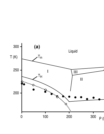
On supercooling water at atmospheric pressure, many thermodynamic and dynamic quantities show power-law growth [1]. This power law behavior also appears under pressure, which allows measurement of the locus of apparent power-law singularities in water [Fig. 1(a)]. The possible explanations of this behavior have generated a great deal of interest. In particular, three scenarios have been considered: (i) the existence of a spinodal bounding the stability of the liquid in the superheated, stretched, and supercooled states [4]; (ii) the existence of a liquid-liquid transition line between two liquid phases differing in density [5, 6, 7]; (iii) a singularity-free scenario in which the thermodynamic anomalies are related to the presence of low-density and low-entropy structural heterogeneities [8]. Based on both experiments [3, 9, 10] and recent simulations [11], several authors have suggested that the power-law behavior of dynamic quantities might be explained by the transient caging of molecules by neighboring molecules, as described by the mode-coupling theory (MCT) [12], which we address here. This explanation would indicate that the dynamics of water are explainable in the same framework developed for other fragile liquids [13], at least for temperatures above the homogeneous nucleation temperature $T_{H}$ . Moreover, this explanation of the dynamic behavior on supercooling may be independent of the above scenarios suggested for thermodynamic behavior [Fig. 1(a)].

Here we focus on the behavior of the diffusion constant $D$ under pressure, which has been studied experimentally [3]. We perform molecular dynamics simulations in the temperature range 210 K – 350 K for densities ranging from 0.95 g/cm³ – 1.40 g/cm³ [Table I] using the extended simple point charge potential (SPC/E) [14]. We select the SPC/E potential because it has been previously shown to display power-law behavior of dynamic quantities, as observed in supercooled water at ambient pressure [11, 15].

In Fig. 2, we compare the behavior of $D$ under pressure at several temperatures for our simulations and the

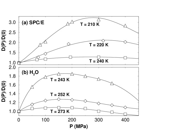
Refer to caption — FIG. 1.: (a) Phase diagram of water. The extrapolated divergence of the isothermal compressibility ( $\circ$ ) [2] and the extrapolated divergence of $D$ (filled $\circ$ ) [3]. The different locations of these divergences suggest that the phenomena may arise from different explanations. (b) Isochrones of $D$ from simulation. The lines may be identified at follows: $D=10^{-5}$ cm²/s ( $\circ$ ); $D=10^{-5.5}$ cm²/s ( $\Box$ ); $D=10^{-6}$ cm²/s ( $\diamond$ ); $D=10^{-7}$ cm²/s ( $\triangle$ ). The diffusion is also fit to $D\sim(T/T_{c}-1)^{\gamma}$ . The locus of $T_{c}$ is indicated by ( $\times$ ). For reference, the ( $+$ ) symbols indicate the locus of T ${}_{\mbox{MD}}$ found in ref. [19].

experiments of ref. [3]. The anomalous increase in $D$ is qualitatively reproduced by SPC/E, but the quantitative increase of $D$ is significantly larger than that observed experimentally. This discrepancy may arise form the fact that the SPC/E potential is under-structured relative to water [19], so applying pressure allows for more bond breaking and thus greater diffusivity than observed experimentally. We also find that the pressure where $D$ begins to decrease with pressure – normal behavior for a liquid – is larger than that observed experimentally. This simple comparison of $D$ leads us to expect that the qualitative dynamic features we observe in the SPC/E potential will aid in the understanding of the dynamics of water under pressure, but will likely not be quantitatively accurate.

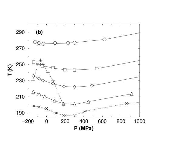
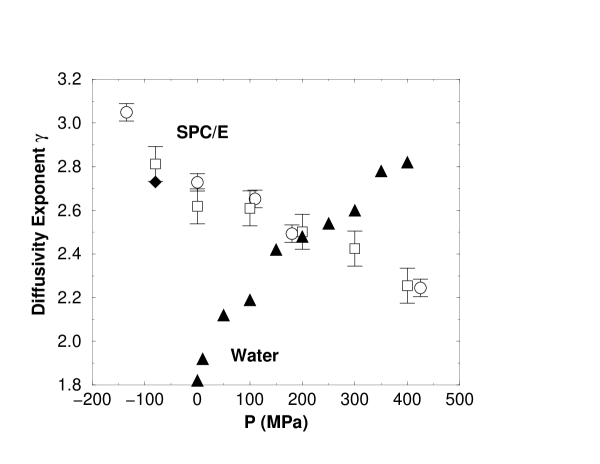
We next determine the approximate form of the lines of constant $D$ (isochrones) by interpolating our data over the region of the phase diagram studied [Fig. 1(b)]. We note that the locus of points where the slope of the isochrones changes sign (i.e. the locus of points where $D$ obtains a maximum value) is close to the $T_{\mbox{MD}}$ locus [19]. At each density studied, we fit $D$ to a power law $D\sim(T/T_{c}-1)^{\gamma}$ . The shape of the locus of $T_{c}$ values compares well with that observed experimentally [3], and changes slope at the same pressure [Figs. 1(a) and (b)]. We find the striking feature that $\gamma$ decreases under pressure for the SPC/E model, while $\gamma$ increases experimentally [Fig. 3]. This disagreement underscores the need to improve the dynamic properties of water models, most of which already provide an adequate account of static properties [21].

We next consider interpretation of our results using MCT, which has been used to quantitatively describe the weak supercooling regime – i.e., the temperature range where the characteristic times become three or

four orders of magnitude larger than those of the normal liquid [22]. The region where experimental data are available in supercooled water is exactly the region where MCT holds. MCT provides a theoretical framework in which the slowing down of the dynamics arises from caging effects, related to the coupling between density modes, mainly over length scales on the order of the nearest neighbors. In this respect, MCT does not require the presence of a thermodynamic instability to explain the power-law behavior of the characteristic times.

MCT predicts power-law behavior of $D$ , and also that the Fourier transform of the density-density correlation function $F(q,t)$ , typically referred to as the intermediate scattering function, decays via a two-step process. $F(q,t)$ can be measured by neutron scattering experiments and is calculated via

F(q,t)\equiv\frac{1}{S(q)}\left\langle\sum_{j,k=1}^{N}e^{-i{\bf q}\cdot[{\bf r}_{k}(t)-{\bf r}_{j}(0)]}\right\rangle,

(1)

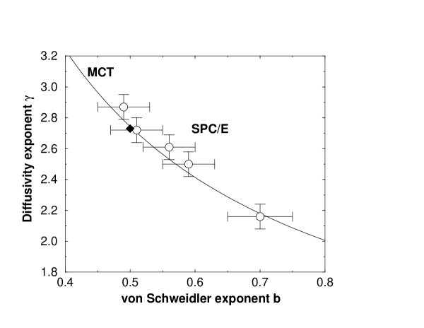
where $S(q)$ is the structure factor [23]. In the first relaxation step, $F(q,t)$ approaches a plateau value $F_{\mbox{plateau}}(q)$ ; the decay from the plateau has the form $F_{\mbox{plateau}}(q)-F(q,t)\sim t^{b}$ , where $b$ is known as the von Schweidler exponent. According to MCT, the value $b$ is completely determined by the value of $\gamma$ [24], so calculation of these exponents for SPC/E determines if MCT is consistent with our results.

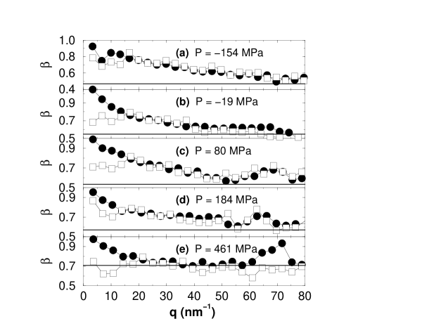
The range of validity of the power-law $t^{b}$ is strongly $q$ -dependent [25], making unambiguous calculation of $b$ difficult. Fortunately, the same exponent $b$ controls the long-time behavior of $F(q,t)$ at large $q$ . Indeed, MCT predicts that at long time, $F(q,t)$ decays according to a Kohlrausch-Williams-Watts stretched exponential

F(q,t)=A(q)\exp{\left[\left(\frac{t}{\tau(q)}\right)^{\beta(q)}\right]},

(2)

with $\lim_{q\to\infty}\beta(q)=b$ [26]. We show the $q$ -dependence of $\beta$ for each density studied at $T=210$ K [Fig. 4]. We also calculate $\beta$ for the “self-part” of $F(q,t)$ , denoted $F_{\mbox{self}}(q,t)$ [27]. In addition, we show the expected value of $b$ according to MCT, using the values of $\gamma$ extrapolated from Fig. 3. The large- $q$ limit of $\beta$ appears to approach the value predicted by MCT [28]. Hence we conclude that the dynamic behavior of the SPC/E potential in the pressure range we study is consistent with slowing down as described by MCT [Fig. 5]. We also note that on increasing pressure, the values of the exponents become closer to those for hard-sphere ( $\gamma=2.58$ and $b=0.545$ ) and Lennard-Jones ( $\gamma=2.37$ and $b=0.617$ ) systems [29]. This confirms that the hydrogen-bond network

is destroyed under pressure and that the water dynamics become closer to that of normal liquids, where core repulsion is the dominant mechanism.

A significant result of our analysis is the demonstration that MCT is able to rationalize the dynamic behavior of the SPC/E model of water at all pressures. In doing so, MCT encompasses both the behavior at low pressures, where the mobility is essentially controlled by the presence of strong energetic cages of hydrogen bonds, and at high pressures, where the dynamics are dominated by excluded volume effects.

We wish to thank A. Rinaldi, S. Sastry, and A. Scala for their assistance. FWS is supported by an NSF graduate fellowship. The Center for Polymer Studies is supported by NSF grant CH9728854 and British Petroleum.

REFERENCES

[1] P. G. Debenedetti, Metastable Liquids (Princeton Univ. Press, Princeton, 1996); C. A. Angell, in Water: A Comprehensive Treatise, edited by F. Franks (Plenum, New York, 1981).
[2] H. Kanno and C.A. Angell, J. Chem. Phys. 70, 4008 (1979).
[3] F.X. Prielmeier, E.W. Lang, R.J. Speedy, and H.-D. Lüdemann, Phys. Rev. Lett. 59, 1128 (1987); Ber. Bunsenges. Phys. Chem. 92, 1111 (1988).
[4] R. J. Speedy and C. A. Angell, J. Chem. Phys. 65, 851 (1976); R. J. Speedy, J. Chem. Phys. 86, 892 (1982).
[5] P. H. Poole et al., Nature 360, 324 (1992); Phys. Rev. E 48, 3799 (1993); Ibid. 48, 4605 (1993); F. Sciortino et al., Ibid 55, 727 (1997); S. Harrington et al., Phys. Rev. Lett. 78, 2409 (1997).
[6] C. J. Roberts, A. Z. Panagiotopoulos, and P. G. Debenedetti, Phys. Rev. Lett. 97, 4386 (1996); C. J. Roberts and P. G. Debenedetti, J. Chem. Phys. 105, 658 (1996).
[7] M.-C. Bellissent-Funel, Europhys. Lett. 42, 161 (1998); O. Mishima and H. E. Stanley, Nature 392, 192 (1998); 396, 329 (1998).
[8] S. Sastry et al., Phys. Rev. E 53, 6144 (1996); L. P. N. Rebelo, P. G. Debenedetti, and S. Sastry, J. Chem. Phys. 109, 626 (1998); H. E. Stanley and J. Teixeira, J. Chem. Phys. 73, 3404 (1980).
[9] A.P. Sokolov, J. Hurst, and D. Quitmann, Phys. Rev. B 51, 12865 (1995).
[10] H. Weingärtner, R. Haselmeier, and M. Holz, J. Phys. Chem. 100, 1303 (1996).
[11] P. Gallo, et al., Phys. Rev. Lett. 76, 2730 (1996); F. Sciortino, et al., Phys. Rev. E 54, 6331 (1996); S.-H. Chen, et al., Ibid 56, 4231 (1997); F. Sciortino, et al., Ibid, 5397 (1997).
[12] W. Götze and L. Sjögren, Rep. Prog. Phys. 55, 241 (1992).
[13] C.A. Angell, Science 267, 1924 (1995).
[14] H. J. C. Berendsen, J. R. Grigera, and T. P. Stroatsma, J. Phys. Chem. 91, 6269 (1987). The SPC/E model treats water as a rigid molecule consisting of three point charges located at the atomic centers of the oxygen and hydrogen which have an OH distance of 1.0 Å and HOH angle of 109.47^∘, the tetrahedral angle. Each hydrogen has a charge $q_{H}=0.4238e$ , where $e$ is the magnitude of the electron charge, and the oxygen has a charge $q_{O}=-2q_{H}$ . In addition, the oxygen atoms of separate molecules interact via a Lennard-Jones potential with parameters $\sigma=3.166$ Å and $\epsilon=0.6502$ kJ/mol.
[15] L. Baez and P. Clancy, J. Chem. Phys. 101, 8937 (1994).
[16] H.J.C. Berendsen et al., J. Chem. Phys. 81, 3684 (1984).
[17] O. Steinhauser, Mol. Phys. 45, 335 (1982).
[18] J.-P. Ryckaert, G. Ciccotti, and H.J.C. Berendsen, J. Comput. Phys. 23, 327 (1977).
[19] S. Harrington et al., J. Chem. Phys. 107, 7443 (1997).
[20] K. Bagchi, S. Balasubramanian, and M. Klein, J. Chem. Phys. 107, 8561 (1997).
[21] SiO₂, another network-forming fluid, confirms the sensitivity of the dynamics on the model potential (M. Hemmati and C.A. Angell, in Physics meet Geology, edited by H. Aoki and R. Hemley (Cambridge Univ. Press, Cambridge, 1998)).
[22] M.D. Ediger, C.A. Angell, and S.R. Nagel, J. Phys. Chem. 100, 13200 (1996).
[23] J.P. Hansen and I. R. McDonald, Theory of Simple Liquids (Academic Press, London, 1986).
[24] W. Götze, in Liquids, Freezing, and Glass Transition, Proc. les Houches, edited by J. P. Hansen, D. Levesque, and J. Zinn-Justin (North-Holland, Amsterdam, 1991).
[25] T. Franosch, M. Fuchs, W. Götze, M.R. Mayr, and A.P. Singh, Phys. Rev. E 55, 7153 (1997).
[26] M. Fuchs, J. Non-Cryst. Solids 172, 241 (1994).
[27] $F(q,t)$ may be split into two contributions: the correlations of a molecule with itself [ $F_{\mbox{self}}(q,t)$ ], and the correlations between pairs of molecules [ $F_{\mbox{distinct}}(q,t)$ ]. We calculate the $q$ -dependence of $\beta$ for $F_{\mbox{self}}(q,t)$ because we have much better statistics for the self-correlations than for cross-correlations.
[28] We confirm that the values of $b$ calculated from $\lim_{q\to\infty}\beta(q)=b$ are consistent with the von Schweidler power-law.
[29] For hard spheres, see J.L. Barrat, W. Götze, and A. Latz, J. Phys. Condensed Matter M1, 7163 (1989); For Lennard-Jones, see U. Bengtzelius, Phys. Rev. A 34, 5059 (1986).

TABLE I.: Summary of the state points simulated. We simulate 216 water molecules interacting via the SPC/E pair potential [14]. We simulate two independent systems at all temperatures (except 350 K), as the large correlation time makes time averaging more difficult. We equilibrate all simulated state points to a constant temperature by monitoring the pressure and internal energy. We control the temperature using the Berendsen method of rescaling the velocities [16] with a thermostat time of 200 ps. The reaction-field technique with a cutoff of 0.79 nm accounts for the long-range Coulomb interactions [17]. The equations of motion evolve using the SHAKE algorithm [18] with a time step of 1 fs. Additional details can be found in ref. [11]. Systems are equilibrated for a time

t_{\mbox{eq}}

, followed by data collection runs for a time

t_{\mbox{data}}

. For all state points, the uncertainty in the potential energy

U

is less the 0.05 kJ/mol.

T	$\rho$ (g/cm³)	U (kJ/mol)	P (MPa)	D ( $10^{-6}$ cm²/s)	$t_{\mbox{eq}}$ (ns)	$t_{\mbox{data}}$ (ns)
210	0.95	$-53.84$	$-154\pm 9$	0.0272	25	50
	1.00	$-53.70$	$-19\pm 11$	0.0913	35	50
	1.05	$-53.43$	$80\pm 12$	0.214	30	50
	1.10	$-53.24$	$184\pm 13$	0.331	30	50
	1.20	$-53.13$	$461\pm 14$	0.290	25	50
220	0.95	$-53.00$	$-150\pm 6$	0.168	15	15
	1.00	$-52.87$	$-21\pm 10$	0.389	15	15
	1.05	$-52.73$	$73\pm 8$	0.558	15	15
	1.10	$-52.59$	$187\pm 8$	0.847	15	15
	1.20	$-52.48$	$480\pm 9$	0.801	15	15
	1.30	$-52.49$	$951\pm 12$	0.263	15	15
240	0.95	$-51.33$	$-153\pm 8$	1.41	7	5
	1.00	$-51.35$	$-45\pm 9$	1.87	7	5
	1.05	$-51.34$	$68\pm 9$	2.44	7	5
	1.10	$-51.28$	$195\pm 10$	2.70	7	5
	1.20	$-51.24$	$527\pm 11$	2.37	7	5
	1.30	$-51.25$	$1035\pm 4$	1.35	7	5
260	0.95	$-49.68$	$-148\pm 9$	5.04	5	3
	1.00	$-49.87$	$-43\pm 10$	6.08	5	3
	1.05	$-49.93$	$77\pm 11$	5.91	5	3
	1.10	$-50.00$	$212\pm 11$	5.88	5	3
	1.20	$-50.10$	$572\pm 13$	5.74	5	3
	1.30	$-50.14$	$1127\pm 14$	3.54	5	3
300	0.95	$-46.80$	$-109\pm 12$	19.9	0.5	1
	1.00	$-47.20$	$-13\pm 13$	20.0	0.5	1
	1.05	$-47.49$	$112\pm 14$	18.3	0.5	1
	1.10	$-47.65$	$264\pm 14$	18.2	0.5	1
	1.20	$-47.95$	$678\pm 16$	15.3	0.5	1
	1.30	$-48.06$	$1293\pm 18$	11.2	0.5	1
350	1.00	$-44.35$	$62\pm 18$	49.7	0.5	40 ps
	1.10	$-45.15$	$358\pm 20$	38.1	0.5	40 ps
	1.20	$-45.56$	$828\pm 22$	27.0	0.5	40 ps
	1.30	$-45.76$	$1504\pm 25$	18.0	0.5	40 ps