The effect of an external magnetic field on the gas-liquid transition in the Ising spin fluid

Abstract

The theoretical phase diagrams of the magnetic (Ising) lattice fluid in an external magnetic field is presented. It is shown that, depending on the strength of the nonmagnetic interaction between particles, various effects of external field on the Ising fluid take place. In particular, at moderate values of the nonmagnetic attraction the field effect on the gas-liquid critical temperature is nonmonotoneous. A justification of such behavior is given. If short-range correlations are taken into account (within a cluster approach), the Curie temperature also depend on the nonmagnetic interaction.

PACS numbers 64.70.Fx, 77.80.Bh, 75.50.Mm, 64.60.Kw.

Anisotropic liquids are very sensitive matters. Such are nematic liquid crystals and ferrofluids. Many efforts have been made in order to investigate effects of shape and flexibility of the molecules, of long and short-range interactions on the properties of anisotropic liquids. External field effects are still worthier of attention, because the application of an external field allows to change properties of anisotropic liquids dynamically (in contrast to the effects of molecules’ shape, etc., which are static).

In ferrofluids an external magnetic field removes the magnetic order-disorder transition, nevertheless the first order transitions between ferromagnetic phases of different densities remain. The external field deforms the phase diagram of a magnetic fluid shifting coexistence lines between these phases. Kawasaki studied a magnetic lattice gas [2], which implements one of the ways to model properties of magnetic fluids. On temperature-density phase diagrams in Ref. [2] one can see that the gas-liquid binodal of the magnetic fluid significantly lowers after the application of an external magnetic field. Vakarchuk with coworkers [3] and Lado et al. [4, 5] studied another model of magnetic fluids — the fluid of hard spheres with embedded Heisenberg spins. They concluded that in such a system the temperature of the gas-liquid critical point (the top of binodal) increases after the application of an external field. The nature of such a discrepancy can be various, because the types of models (continuum fluids [3, 4, 5] and the lattice gas [2]) as well as approximations used differ.

In this letter results of a more detailed investigation of the magnetic (Ising) lattice gas are reported. The first new point is the inclusion of the nonmagnetic interaction between particles. Another one consists in overcoming of limitations applied by the mean field approximation (MFA). It is known that this approximation is good for very long-range potentials only (and becomes accurate for a family of the infinite-ranged ones, the so-called Kac potentials [6, 7]). The MFA can not reproduce some essential features of the systems with the nearest-neighbor interaction (such as the percolation phenomena in the quenched diluted Ising model, differences in magnetic properties of the quenched site-disordered Ising model and the annealed one [8]). Such drawbacks can be overcome with the two-site cluster approximation (TCA) [9].

We shall show within both the MFA and the TCA that at different values of the nonmagnetic interaction between particles the Ising fluid demonstrates various effects of external fields. In particular, at moderate values of the nonmagnetic attraction the field effect on the critical temperature is nonmonotoneous.

In lattice models of a fluid its particles are allowed to occupy only those spatial positions which belong to sites of a chosen lattice. The configurational integral of a simple fluid is in such a way substituted by the partition function

$$Z=\mbox{Sp}\exp\left(-\beta{\cal H}\right),~{}\beta=1/(k_{\rm B}T),$$ (1)

$${\cal H}=H-\mu N=-\frac{1}{2}\sum_{ij}I_{ij}n_{i}n_{j}-\mu\sum_{i}n_{i},$$ (2)

where $n_{i}$, which equals 0 or 1, is a number of particles at site $i$. Sp means a summation over all occupation patterns. The total number $N$ of particles is allowed to fluctuate, $\mu$ is a chemical potential, which should be determined from the relation

$$N=\left\langle\sum_{i}n_{i}\right\rangle_{{\cal H}};~{}\left\langle\cdots\right\rangle_{{\cal H}}=Z^{-1}\mbox{Sp}(\cdots)\exp(-\beta{\cal H}).$$ (3)

Lattice models, due to particles can not approach closer than the lattice spacing allows, automatically preserve the essential feature of molecular interaction: nonoverlapping of particles. The lattice fluid with nearest neighbor interaction is known to demonstrate the gas-liquid transition only. Nevertheless, the lattice gas with interacting further neighbors possesses a realistic (that means, argon-like) phase diagram with all transitions between the gaseous, liquid and solid phases being present [10].

We shall consider a magnetic fluid in which the particles carry Ising spins $S_{i}=\pm 1$ and there is also an additional exchange interaction between the particles

$$H-\mu N = -\frac{1}{2}\sum_{ij}J_{ij}S_{i}n_{i}S_{j}n_{j}-h\sum_{i}S_{i}n_{i}$$ (5)

$$-\frac{1}{2}\sum_{ij}I_{ij}n_{i}n_{j}-\mu\sum_{i}n_{i}$$

Each site can be in three states: empty (i), occupied by the particle with spin up (ii) or down (iii). The trace in the partition function implies a summation over all $3^{\cal N}$ states, where ${\cal N}$ is a number of sites.

An interaction of fluctuations are totally neglected in the mean field approximation used in the previous studies of the model [2]. This can partially be recovered using the idea of “clusters”. The partition function of a finite group of particles in an external field can be evaluated explicitly. A contribution of the other particles may be expressed in terms of the effective field, and this field has to be evaluated selfconsistently. From such a point of view the MFA is a one-site cluster approximation, in which each cluster comprises one site. Increasing the size of clusters one may expect to obtain more accurate results. Indeed, the results of the two-site cluster approximation turns to be accurate for the one-dimensional systems [11] and on the Cayley tree [8]. Here we shall formulate such an approximation for the Ising lattice gas with the nearest neighbor interactions. For the sake of brevity we shall not use the cluster expansion formulation which has some advantages, such as the possibility to calculate corrections of a higher order and correlation functions of the model [9]. Instead we shall rely on the first order approximation and closely follow the derivation by Vaks and Zein [8]. Let us introduce the effective-field Hamiltonian of a single site

$$H_{i}-\mu n_{i}\equiv{\cal H}_{i}=-\tilde{h}S_{i}n_{i}-\tilde{\mu}n_{i},$$ (6)

where $\tilde{h}=h+z\varphi$, $\tilde{\mu}=\mu+z\psi$, $\varphi$ and $\psi$ are effective fields substituting for interactions with nearest neighbor sites, $z$ is a first coordination number of the lattice. In the two-site Hamiltonian the interaction between a pair of the nearest neighbor sites is taken into account explicitly

$$H_{ij}-\mu n_{i}-\mu n_{j}\equiv{\cal H}_{ij} = -J_{ij}S_{i}n_{i}S_{j}n_{j}-\tilde{h}^{\prime}S_{i}n_{i}-\tilde{h}^{\prime}S_{j}n_{j}$$ (8)

$$-I_{ij}n_{i}n_{j}-\tilde{\mu}^{\prime}n_{i}-\tilde{\mu}^{\prime}n_{j},$$

where $\tilde{h}^{\prime}=h+z^{\prime}\varphi$, $\tilde{\mu}^{\prime}=\mu+z^{\prime}\psi$, and $z^{\prime}=z-1$ due to one of the neighbors is already taken into account. The fields have to be found from the selfconsistency conditions that require an equality of average values calculated with the one-site and two-site Hamiltonians. To determine $\varphi$ and $\psi$ it is sufficient to impose these conditions on the average values of spin $m=\left\langle S_{i}n_{i}\right\rangle_{{\cal H}}$ and of the occupation number $n=\left\langle n_{i}\right\rangle_{{\cal H}}$,

$$\left\langle n_{i}\right\rangle_{{\cal H}_{i}}=\left\langle n_{i}\right\rangle_{{\cal H}_{ij}};~{}\left\langle S_{i}n_{i}\right\rangle_{{\cal H}_{i}}=\left\langle S_{i}n_{i}\right\rangle_{{\cal H}_{ij}}.$$ (9)

This approximation leads to the following expression for the internal energy

$$U/{\cal N} = -\frac{1}{2}J_{0}\left\langle S_{i}n_{i}S_{j}n_{j}\right\rangle_{{\cal H}_{ij}}-h\left\langle S_{i}n_{i}\right\rangle_{{\cal H}_{ij}}$$ (11)

$$-\frac{1}{2}I_{0}\left\langle n_{i}n_{j}\right\rangle_{{\cal H}_{ij}},$$

where $J_{0}=\sum_{j}J_{ij}=zK$ and $I_{0}=\sum_{j}I_{ij}=zV$ are integral interaction strengths, $K$ and $V$ denote, respectively, the magnetic coupling and the nonmagnetic attraction between nearest neighbor sites. The expression (11) can be computed explicitly in terms of the fields $\varphi$ and $\psi$ and model parameters. The other thermodynamic potentials can be found in a straightforward way. For example, the grand thermodynamic potential $\Omega$ of the model satisfies the following Gibbs-Helmholtz equation

$$\frac{\partial\beta\Omega}{\partial\beta}=U-\mu N.$$ (12)

The solution of this differential equation, taking into account relations (9), reads

$$\beta\Omega/{\cal N}=z^{\prime}\ln\mbox{Sp}\exp(-\beta{\cal H}_{i})-\frac{z}{2}\ln\mbox{Sp}\exp(-\beta{\cal H}_{ij}).$$ (13)

It is possible to build isotherms of the fluid using the thermodynamic relation $\Omega=-PV$ and expression (13) and solving the system of nonlinear selfconsistency equations (9). It is possible and convenient to exclude the chemical potential $\mu$ and the field $\psi$ from final equations of state:

$$\beta PV/{\cal N} = -\ln(1-n)+\frac{z}{2}\ln[(1-n)(1-x)+xr],$$ (14)

$$\tanh\beta\tilde{h} = p\frac{\sinh 2\beta\tilde{h}^{\prime}}{\cosh 2\beta\tilde{h}^{\prime}+\exp(-2\beta K)}$$ (16)

$$+(1-p)\tanh\beta\tilde{h}^{\prime},$$

where

$$p = 1-(1-n)/r,~{}r=0.5+\sqrt{(n-0.5)^{2}+n(1-n)/x},$$ (17)

$$x = \frac{2\exp(-\beta V-\beta K)\cosh^{2}\beta\tilde{h}^{\prime}}{\cosh 2\beta\tilde{h}^{\prime}+\exp(-2\beta K)},$$ (18)

$p$ is a probability that a randomly chosen nearest neighbor site to a given particle is occupied. In the limit $z\to\infty$ and $K\to 0$, $V\to 0$ (keeping $J_{0}$ and $V_{0}$ constant) TCA formulae (14–18) turn into the results of the MFA.

At low temperatures the isotherms of the fluid contain the “liquid” and “gaseous” parts separated by a region of the negative compressibility. The thermodynamic states, in which the compressibility of the uniform fluid is negative ($\frac{\partial P}{\partial n}<0$), constitute the spinodal region on the temperature-density phase diagram. In this region the fluid is thermodynamically unstable and must separate on phases of different densities. The densities of coexisting phases can be determined with the Maxwell rule of areas applied to the nonmonotoneous sections of the isotherms. Also at sufficiently low temperatures and $h=0$ an isotherm of the model has a break at the density in which nonzero solution of selfconsistency equation (16) for the field $\varphi$ appears, and the second order phase transition to the ferromagnetic phase occurs.

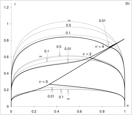
FIG. 1.: The phase diagram of the magnetic (Ising) lattice gas within the mean field (a) and two-site cluster (b) approximations. $n=N/{\cal N}$ and $t=k_{\rm B}T/J_{0}$ are reduced density and temperature, respectively. Picture b represents TCA results for the model with the nearest neighbor interactions on the simple cubic lattice ($z=6$). The results of MFA (picture a) are independent of interaction range and lattice structure. Three families of lines are built for three values of nonmagnetic interaction $v=I_{0}/J_{0}$. The thick lines are binodals and Curie lines at zero external field. The thin lines with attached numbers represent the binodals at nonzero values of the external field $h/J_{0}$.

Figure 1a shows the temperature-density phase diagram of the model within the mean field approximation at different model parameters. There are three families of lines for three values of the nonmagnetic interaction strength $v=I_{0}/J_{0}$. The bold lines correspond to zero field case ($h=0$). The straight line is a line of Curie points that separates paramagnetic and ferromagnetic regions. Within the mean field approximation the slope of the Curie line is independent of $v$. Under binodals (convex lines resting on the points (0,0) and (1,0) on the phase diagram) a phase separation takes place: one of the phases (vapor) is rarefied, the other (liquid) is denser. The nonmagnetic attraction between particles, of course, favors the phase separation — the binodal moves upward with increasing $v$. At small $v$ the phase diagram possesses of the tricritical point: the top of binodal lays on the Curie line, the liquid is ferromagnetic and the gas is paramagnetic. The tricritical point disappears at large $v$, in this case the top of binodal deviates from the Curie line in the paramagnetic region.

The external field dissolves the ferromagnetic transition and therefore eliminates the Curie line. The gas-liquid binodals in presence of the external magnetic field are depicted with thin lines. The attached numbers are strengths of the field $h/J_{0}$. At small $v$ there is a temperature interval, where the external field suppresses phase separation — the top of binodal shifts downward in agreement with the results of Kawasaki [2]. Nevertheless, at large nonmagnetic attractions (e.g., $v=4$) the reverse field effect takes place. At moderate values of the nonmagnetic interaction (for example, $v=2$) the field effect is nonmonotoneous — weak fields lower the top of binodal, stronger fields shift it up.

In Fig. 1b one can see that the TCA, besides quantitative differences, gives some qualitative corrections to the MFA results. Within the TCA the Curie line becomes slightly concave, and the nonmagnetic attraction between particles increases the Curie temperature. The latter effect can be justified by the qualitative arguments. Indeed, the nonmagnetic attraction increases the probability that a randomly chosen pair of the nearest neighbor sites is occupied. Since at this sites particles interact magnetically, the magnetic interaction becomes more effective, and the Curie temperature increases also. Therefore the account of density fluctuations in the TCA leads to the dependence of the Curie temperature on $v$. In the case of the non-compressible fluid ($n=1$) the density fluctuations are absent, and the Curie temperature is independent of the nonmagnetic attraction.

The TCA predictions concerning the effect of field support the MFA results. The variety of field effects may be explained by the existence of two concurrent tendencies. The first, the external field aligns the spins, which leads to the more effective attraction between particles (let us remind that at $v=0$ particles with parallel spins ($S_{i}S_{j}=1$) attract and those with opposite spins ($S_{i}S_{j}=-1$) repulse). This raises the binodal (for example, in simple nonmagnetic fluids the binodal goes up when the interaction increases). The second tendency takes place, if the susceptibility of the rarefied phase is larger than that of the coexisting dense phase. In this case the magnetization and, consequently, the effective attraction between particles grow better in the rarefied phase. This decreases the energetical gain of the phase separation. Therefore the second tendency suppresses the gas-liquid separation in the fluid and counteracts the first tendency. The second tendency is very strong at $h=0$ and $v=0$ in the region of the tricritical point, where the vapor (paramagnetic) branch of binodal almost coincides with the Curie line (where the susceptibility tends to infinity), whereas the branch of the coexistent liquid phase rapidly deviates from the Curie line. As a result, the external field lowers the top of the binodal. The second tendency gets weak and disappears when the susceptibilities of the coexistent phases levels; they are comparable, for example, if both liquid and vapor phases are paramagnetic. The behavior of $v=4$ binodal (see Fig. 1) demonstrates this feature. A relation between the susceptibilities results from various factors. For example, a short-rangeness of the interactions levels the susceptibilities and weakens the second tendency [12]. It can be seen from the following observation of the field effect at $v=2$: in Fig. 1a the top of binodal at $h=0.01$ is higher than that at $h=0.1$, whereas in Fig. 1b the reverse situation takes place. Since the results of the MFA (as well as those of the TCA in the limit $z\to\infty$) are correct for the long-ranged potentials, whereas for our case the TCA is much more accurate, the corrections provided by the TCA have to be attributed to differences between the systems with the long-range and short-range potentials.

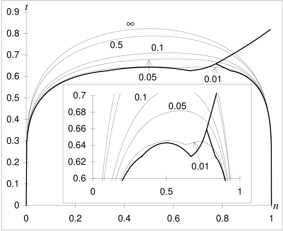
FIG. 2.: The phase diagram of the model at $v=3$ within the TCA. The inset shows the vicinity of the top of $h=0$ binodal in a more detail.

Still more illuminating confirmation of the “bi-tendency” explanation one can see in Fig. 2. There is the phase diagram of special topology, which takes place at intermediate $v$. The model at $h=0$ and $t=0.63$ undergoes two first-order phase transitions. At this temperature the fluid can be in three phases: paramagnetic gas (at $n<0.35$), paramagnetic liquid ($0.65<n<0.69$), ferromagnetic liquid ($n>0.83$). What we would like to emphasize is that weak external fields (e.g., $h/J_{0}=0.01$) raise the binodal at $n=0.5$ and lower it at $n=0.75$. Such behavior completely fit into the “bi-tendency” explanation: at $n=0.5$ and $h=0$ both phases are paramagnetic, the second tendency is absent, therefore the external field favors the phase separation; at $n=0.75$ the second tendency wins at small fields, like in the case $v=2$ (see Fig. 1).

One can see that the lattice gas approach may be successfully used for description of complex fluids when continual approaches lead to too complex calculations or do not give satisfactory results. It is this situation that takes place when one determines the influence of the nonmagnetic attraction on the Curie temperature [12, 13]. In this case the account of the short-range correlations within the cluster approach yields qualitatively new results in comparison with current continual methods.

REFERENCES

- [1] E-mail: ccc@icmp.lviv.ua
- [2] T. Kawasaki, Progr. Theor. Phys. 58, 1357 (1977).
- [3] I.O. Vakarchuk, H.V. Ponedilok, and Yu.K. Rudavskii, Teor. Mat. Fiz. 58, 445 (1984).
- [4] F. Lado, E. Lomba, and J. J. Weis, Phys. Rev. E 58, 3478 (1998).
- [5] F. Lado and E. Lomba, Phys. Rev. Lett. 80, 3535 (1998).
- [6] J. Lebovitz, O. Penrose, J. Math. Phys. 7, 1016 (1966).
- [7] R. Balescu, Equilibrium and nonequilibrium statistical mechanics (Wiley, New-York, 1975), Chap. 9.4
- [8] V.G. Vaks, N.Ye. Zein, Zh. Eksp. Teor. Fiz. 67, 1082 (1974).
- [9] R.R. Levitskii, S.I. Sorokov, R.O. Sokolovskii, Acta Physica Polonica A 92, 383 (1997).
- [10] C.K. Hall and G. Stell, Phys. Rev. A7, 1679 (1973).
- [11] B.Ja. Balagurov, V.G. Vaks, R.O. Zajtsev, Fiz. Tverd. Tela 16, 2302 (1974).
- [12] T.G. Sokolovska, R.O. Sokolovskii, cond-mat/9810244.
- [13] B. Groh and S. Dietrich, Phys. Rev. Lett. 72, 2422 (1994)