[

Path Crossing Exponents and the External Perimeter in 2D Percolation

Abstract

$2$D Percolation path exponents $x^{\cal P}_{\ell}$ describe probabilities for traversals of annuli by $\ell$ non-overlapping paths, each on either occupied or vacant clusters, with at least one of each type. We relate the probabilities rigorously to amplitudes of $O(N=1)$ models whose exponents, believed to be exact, yield $x^{\cal P}_{\ell}=({\ell}^{2}-1)/12$. This extends to half-integers the Saleur–Duplantier exponents for $k=\ell/2$ clusters, yields the exact fractal dimension of the external cluster perimeter, $D_{EP}=2-x^{\cal P}_{3}=4/3$, and also explains the absence of narrow gate fjords, as originally found by Grossman and Aharony.

]

The fractal geometry of critical percolation clusters has been of interest both for intrinsic reasons and as a window on a range of phenomema. It is characterized by fractal dimensions of various sets [1, 2], e.g., of the connected clusters, their backbones, the sets of pivotal (singly–connecting) bonds, the clusters’ boundaries (hulls), and their external (accessible) perimeters. A set $S$ is said here to be of fractal dimension $D_{S}$ if the density of points in $S$ within a box of linear size $R$ decays as $R^{-x_{S}}$, with $x_{S}=d-D_{S}$ in $d$ dimensions.

For two–dimensional (2D) independent percolation, many of the fractal dimensions have been found exactly [3, 4, 5, 6], though most of these values have not yet been established at a rigorous level. In several cases, Saleur and Duplantier (SD)[5] identified the co–dimension $x_{S}$ with the exponent $x^{\cal C}_{k}$ which describes the decay law $P^{\cal C}_{k}\approx(r/R)^{x^{\cal C}_{k}}$ for the probability ($P^{\cal C}_{k}$) that in an annular region $D(r,R)$ the small circle of radius $r$ is connected to the outer one, of radius $R>>r$, by $k$ different clusters of occupied sites (or bonds). SD utilized the observation that the statistics of the $2k$ boundary lines of the connected clusters correspond to those of loops in some well recognized models: the $Q=1$ Potts model (at its critical point) for the bond percolation model and the $O(N=1)$ loop model of Domany et al.[7] (at its low temperature phase) for site percolation on the triangular lattice. Using the “Coulomb gas” representation for the corresponding $\ell$-line exponents, $x^{O(N)}_{\ell}$, SD obtained [5] for both models the values, expected to be universal,

$$x^{\cal C}_{k}=x^{O(N=1)}_{\ell=2k}=(4k^{2}-1)/12\;,$$ (1)

where $k$ clusters correspond to $\ell=2k$ lines in the loop model.

Among the noteworthy applications of the above formula are the “hull dimension”, i.e., the dimension of the cluster’s perimeter,

$$D_{H}=2-x^{\cal C}_{1}=7/4,$$ (2)

and the dimension of the set of “red” (singly connecting) bonds, which are pinching points between two large clusters:

$$D_{SC}=2-x^{\cal C}_{2}=3/4=1/{\nu},$$ (3)

where $\nu$ is the correlation length exponent [8], in agreement with previously derived values [3]. However, some well known percolation dimensions have eluded this exact approach: the dimension $D_{EP}$ of the external (accessible) perimeter (EP) or frontier of a cluster, first studied by Grossman and Aharony (GA)[9], and the backbone dimension. The EP of a cluster is the accessible part of the hull, which excludes deep “fjords” which are connected to the cluster’s complement through very narrow passages (or “gates”). The dimension of the EP was found numerically to be $D_{EP}\approx 4/3$ [10]. GA [9] also made the puzzling observation that, while typical clusters do show many fjords with only a narrow passage to the complement, once one fills in fjords with passages of width two or three lattice spacings – no fjords of broader microscopic passages, and depth comparable with that of the cluster, are left. This is clearly visible in Fig. 6 of the second Ref. [9]. Both of these observations make the EP look very similar to self–avoiding walks (SAW’s). Although there appeared conjectures attempting to make this relation quantitative [5, 9], the connection was never elucidated.

In this Letter we report on a resolution of these issues through analysis of the path crossing probabilities.

i. Basing the relation of percolation exponents with the $O(N=1)$ exponents on a somewhat different footing than that used in Ref.[5], we extend the list of exact values proposed for critical percolation in 2D. Instead of focusing on entire clusters, we consider the probability $P^{\cal P}_{\ell}(r,R;\tau_{1},\ldots,\tau_{\ell})$ that the annulus $D(r,R)$ is traversed by (at least) $\ell$ non–overlapping connected paths, which are “monochromatic” in the sense that each consists of either occupied sites (“color” $\tau_{j}=+$) or vacancies ($\tau_{j}=-$). We rigorously prove [11] that for color sequences which include at least one of each type ($\pm$) the decay rates of the probabilities are color-independent, and are given by the $O(N=1)$ exponents. Assuming the validity of the exact values for the latter, we find that

$$P^{\cal P}_{\ell}(r,R;\tau_{1},\ldots,\tau_{\ell})\approx(r/R)^{x^{\cal P}_{\ell}}$$ (4)

with the path crossing exponents $x^{\cal P}_{\ell}$ satisfying

$$x^{\cal P}_{\ell}=x^{O(N=1)}_{\ell}=(\ell^{2}-1)/12.$$ (5)

Since the cluster exponents are $x^{\cal C}_{k}=x^{\cal P}_{2k}$, Eq. (5) may be viewed as an extension of the SD formula to odd values of $\ell$, or half integer values of $k$, and to more general sequences $\tau_{j}=\pm$.

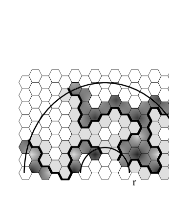
FIG. 1.: A configuration with $\ell=2$ paths traversing the semi-annular region $\tilde{D}(r,R)$, one of occupied (checkered) and the other (dual) of vacant (gray) hexagons. The configuration has $(\ell+1=3)$ $\ O(N=1)$ boundary lines (drawn thickly); the states of the hexagons not adjacent to these lines are left unspecified.

ii. Using the newly acquired values we explain some of the quantitative and qualitative features of the EP of critical clusters mentioned above: its dimension, which we identify as

$$D_{EP}=2-x^{O(1)}_{3}=4/3\;,$$ (6)

and the interesting fact that – unlike the hull – the EP appears to be self–avoiding on the macroscopic scale.

iii. We consider also the analogous boundary or “surface” exponents, which describe the probability $\tilde{P}^{\cal P}_{\ell}(r,R;\tau_{1},\ldots,\tau_{\ell})$ that, within the upper half space, a semi-annular region $\tilde{D}(r,R)$ is traversed by $\ell$ paths (see Fig. 1). For the exponents defined by

$$\tilde{P}^{\cal P}_{\ell}(r,R;\tau_{1},\ldots,\tau_{\ell})\approx(r/R)^{\tilde{x}^{\cal P}_{k}}$$ (7)

we find

$$\tilde{x}^{\cal P}_{\ell}=\tilde{x}^{O(N=1)}_{\ell+1}=(\ell+1)\ell/6.$$ (8)

In this case the relation is valid with no restriction on the color sequence $\tau$; however there is a shift: $\ell$ crossing paths correspond to $(\ell+1)$ $O(N=1)$ lines. Thus, with odd $\ell$, one recovers the cluster boundary exponents $\tilde{x}^{\cal C}_{k}=\tilde{x}^{\cal P}_{2k-1}=k(2k-1)/3$, as in Refs. [12, 13].

Before we turn to describe the arguments for the exact values of the path exponents, as provided by Eqs. (5) and (8), let us present their implications concerning the dimension and shape of the external perimeter. Each point on the accessible EP is next to the end of three paths of lengths comparable with the diameter of the cluster – a path of occupied sites and in addition two distinct dual paths of vacancies (Fig. 2a), which guarantee that the point is not within a fjord of narrow opening (both paths must be able to exit the fjord via the narrow gate). This yields $D_{EP}\ =\ 2-x^{\cal P}_{3}=4/3,$ in excellent agreement with the numerical results[10].

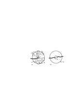
FIG. 2.: Paths, and dual (dotted) paths characterizing a) the external perimeter ($\ell=3$) and b) a gate ($\ell=6$).

GA’s observation concerning the fjords is particularly striking from the perspective of the scaling limit, for which one sends the lattice spacing to zero while keeping the sight on the curves observed on the macroscopic scale. (The limit can be constructed using the analysis of Ref. [14], which implies that the cluster hulls and EP’s can still be described by means of Hölder continuous random curves.) While the EP is self–avoiding on the lattice scale, like the hull it could have close encounters which appear as self–intersections when viewed from the macroscopic perspective. Yet such close encounters are not observed. Also this puzzle is explained by the generalized path statistics: the occurence in an $L\times L$ box of a cluster with a fjord of depth $R=sL$ and neck width $r=\epsilon L$ requires there being six paths, two pairs of triplets as used in the derivation of Eq. (6), which meet in a region of size $r$ and avoid each other up to a radius $R$ (Fig. 2b). The probability of finding such six paths scales as $\epsilon^{-d}\times\left({\epsilon\over s}\right)^{x^{\cal P}_{6}}\ =\ O(\epsilon^{x^{P}_{6}-d})$ where $d=2$. Equation (5) yields the exponent value $x^{\cal P}_{6}=2{11\over 12}$ and hence the probability for a randomly picked configuration to exhibit such a gate tends to zero, in the situation where $s$ is fixed at some non-infinitesimal value $0<s<1$, and $\epsilon\to 0$. The crucial point here is that the fractal dimension of the set of these gates is negative:

$$D_{G}\ =\ 2-x^{\cal P}_{6}\ <\ 0\;.$$ (9)

This explains the asymptotic absence of macroscopic size fjords of neck width $r$ anywhere between few multiples of the lattice spacing and $\epsilon L$, for any fixed $\epsilon\ll 1$. The above argument also implies that the EP will not exhibit peninsulas with narrow isthmuses, even though that condition was not built into the construction.

It is of interest to recall here the suggestion which was made on a theoretical as well as a numerical basis [15, 16], that percolation’s hull and EP dimensions coincide with the dimensions of polymers, respectively at the $\theta$-point (the onset of collapse), or in the SAW state:

$$D_{H}=D_{\theta},\quad D_{EP}=D_{SAW}\;.$$ (10)

It is natural to conjecture that in the scaling limit the EP coincides, in its local statistics, with a SAW. This may appear to be in conflict with the a-symmetry between the two sides of the EP, however the absence of peninsulas in the scaling limit suggests that the symmetry is restored asymptotically.

The above results (5-9) are based on a rigorous relation of path crossing probabilities with amplitudes of a loop model which we shall now define, and on known exact values for the exponents of the latter (which still remain to be proven at a rigorous level). The arguments, which will be presented more completely in ref. [11], are formulated for the special model of independent site (i.e., hexagon) percolation on the triangular lattice. For reasons of universality one may expect the conclusions to apply to other 2D percolation models, e.g., the bond percolation, and also to the statistics of the connected clusters of ($+$) or ($-$) spins in the 2D Ising model at all temperatures above $T_{c}$.

The loop-model configurations, $\Gamma$, are collections of nonoverlapping loops and lines, in suitable subsets of the plane, which are allowed to have end-points only within prescribed regions. The weight of a configuration is

$$W(\Gamma)\ =\ K^{\cal N_{B}}N^{\cal N_{P}}\;,$$ (11)

with ${\cal N_{P}}$ the number of closed lines (or “polygons”) and ${\cal N_{B}}$ their total length (the number of bonds). For the particular case of hexagon percolation discussed here the fugacities are $K=1$, $N=1$, i.e., $W(\Gamma)=1$ for all $\Gamma$ [5].

A probability distribution of loop and line configurations in a prescribed region is defined by means of the weights $W(\Gamma)/Z$, with $Z$ a suitable normalizing factor. Let now $P^{O(N)}_{\ell}(r,R)$ denote the probability that such a system of lines with no end points in the annular domain $D(r,R)$ contains at least $\ell$ lines traversing $D(r,R)$. For a representation of the surface exponents, we also let $\tilde{P}^{O(N)}_{\ell}(r,R)$ denote the corresponding event with the lines restricted to lie in the upper half plane, taken here with the “free boundary conditions”. A close variant of the quantity $P^{O(N)}_{\ell}(r,R)$ is the $O(N)$ amplitude $G^{O(N)}_{\ell}(r,R)$ which is defined as the sum over $\ell$ lines $\{\gamma_{1},\ldots,\gamma_{\ell}\}$ spanning the annulus $D(r,R)$ of the probability $\omega(\gamma_{1},\ldots,\gamma_{\ell}\in\Gamma)$ that the lines are included in $\Gamma$. For $N=1$, that probability reduces to the local expression[16, 11]:

$$\omega(\gamma_{1},\ldots,\gamma_{\ell}) = 2^{-{\cal N}_{H}(\gamma_{1},\ldots,\gamma_{\ell})}2^{{\cal K}(\gamma_{1},\ldots,\gamma_{\ell})}/2^{\#}$$ (12)

with ${\cal N}^{H}(\gamma_{1},\ldots,\gamma_{\ell})$ the number of hexagons touched by the lines, ${\cal K}(\gamma_{1},\ldots,\gamma_{\ell})$ the number of line clusters – two lines being regarded as in the same cluster if they touch a common hexagon, and $\#$ defined as taking the value $0$ if the $\ell$ lines leave room for another curve to traverse the annulus and $1$ otherwise. The amplitudes then read

$$G^{O(N=1)}_{\ell}(r,R)\ =\ \sum_{\gamma_{1},\ldots,\gamma_{\ell}}\omega(\gamma_{1},\ldots,\gamma_{\ell}),$$ (13)

the sum running over sets of $\ell$ nonoverlapping lines which traverse $D(r,R)$. It can be shown that the probabilities and amplitudes agree to the leading order [11]:

$$P^{O(N=1)}_{\ell}(r,R)\ =\ \left(1+o({r\over R})\right)G^{O(N=1)}_{\ell}(r,R)\;.$$ (14)

“Coulomb gas” and Bethe Ansatz methods [4, 5, 17, 18, 19] yield the conclusion that the loop model amplitudes, and thus also the probabilities, decay by power laws, $G^{O(1)}_{\ell}(r,R)\approx(r/R)^{x^{O(1)}_{\ell}}$, and $\tilde{G}^{O(1)}_{\ell}(r,R)\approx(r/R)^{\tilde{x}^{O(1)}_{\ell}}$, with the exponents taking the values given in Eq. (5) and Eq. (8). Our results rest now on the fact that the $O(N=1)$ line probabilities are of the same order of magnitude as the path crossing probabilities. Their compatibility is expressed in the following statement.

Proposition In the site percolation model on the triangular lattice:

1) For any “color sequence” $\{\tau_{j}=\pm\}_{j=1}^{\ell}$ which includes at least one of each kind ($+$ and $-$),

$$P^{\cal P}_{\ell}(r,R;\tau_{1},\ldots,\tau_{\ell})\ \ {\stackrel{{\scriptstyle\scriptstyle<}}{{{}_{{}_{\scriptstyle>}}}}}\ \ P^{O(N=1)}_{\ell}(r,R)\;,$$ (15)

where $A\ {\stackrel{{\scriptstyle\scriptstyle<}}{{{}_{{}_{\scriptstyle>}}}}}\ B$ means that there are constants $0<c_{1},c_{2}<\infty$ with which $c_{1}A\leq B\leq c_{2}A$ uniformly in $r$ and $R$.

2) The surface probabilities satisfy

$$\tilde{P}^{\cal P}_{\ell}(r,R;\tau_{1},\ldots,\tau_{\ell})\ =\ \tilde{P}^{O(N=1)}_{\ell+1}(r,R)\;,$$ (16)

without any restriction on the color sequence $\tau$.

Let us outline here the proof, whose details will be spelled in ref. [11]. The simplest case of the above relation is in the example of the half-disk amplitude with alternating color paths (as in Fig. 1), which corresponds to $\tilde{P}^{\cal P}_{\ell}(r,R;+,-,+,-,\ldots)$. Equation (16) holds there since the statistics of the boundary lines is given exactly by the $O(N=1)$ loop model. The result is then extended by establishing independence on the color sequence. This is done by successively conditioning on the suitable “rightmost path” and flipping the site variables left of the line. Thus use is made of the Markov property combined with the spin flip symmetry, which are enabled by the independence and the self duality of the site percolation model on the triangular lattice. The argument is a bit more involved in the case of the full disk. There we need to have at least one traversing boundary line, which we employ to slit the annulus. The previous argument is then applied to the resulting simply connected domain. Equation  (15) reflects the fact that the overcounting involved in the selection of the slit is by at most a finite factor.

As noted in [20, 21], it is possible to obtain some selected path exponents by direct arguments. The values agree with the formulas given above. It is instructive to list specific values of $x^{\cal P}_{\ell}=(\ell^{2}-1)/12$:
$\ell=2$:  $x^{\cal P}_{2}$ yields $D_{H}=D_{\theta}=7/4$.
$\ell=3$:  $x^{\cal P}_{3}$ yields $D_{EP}=D_{SAW}=4/3$.
$\ell=4$:  $x^{\cal P}_{4}$ yields $D_{SC}=\nu^{-1}=3/4$.
$\ell=5$:  $x^{\cal P}_{5}=2$ can be derived directly.
$\ell=6$:  $x^{\cal P}_{6}>2$ implies that the EP is self–avoiding on the large scale ($D_{G}<0$).

The relation (5) was not claimed for $\ell=1$, or for paths of a single color ($\hat{x}^{\cal P}_{\ell}$). Concerning this let us note:
     – It can be shown directly that $x^{O(N=1)}_{1}=0$ [11] while $\hat{x}^{\cal P}_{1}>0$ [22]. The path exponent is related to the cluster dimension; its value appears to be $\hat{x}^{\cal P}_{1}=5/48$ [3].
     – The case of $\ell=2$, with two paths of the same color, is of special interest since it relates to the backbone dimension. Numerically, $\hat{x}^{\cal P}_{2}=0.3568\pm 0.0008$ [23].

For the surface exponents, $\tilde{x}^{\cal P}_{\ell}=(\ell+1)\ell/6$ of Eq. (8), we note that for $\ell\to\infty$  $\tilde{x}^{\cal P}_{\ell}/x^{\cal P}_{\ell}\to 2$, as it should; and $\ell=1$:  $\tilde{x}^{\cal P}_{1}=1/3\ \$ is consistent with Cardy’s equation for the crossing probability [6].
$\ell=2$:  $\tilde{x}^{\cal P}_{2}=1$ can be derived directly.
$\ell=3$:  $\tilde{x}^{\cal P}_{3}=2$ is also directly derivable.
The last one [21] is related to a slit-disc exponent which is attributed to J. van den Berg in Ref. [20].

Finally, we note that the SD formalism also yields predictions for the hull dimensions of Fortuin-Kasteleyn random clusters, describing the $Q$-state Potts model. These were recently confirmed in numerical simulations by Hovi and Mandelbrot [24]. In contrast, the values found in that work for the external perimeters do not agree with the generalizations of the SD formulas to odd $\ell$. The results presented here were derived only for site percolation. It would be interesting to see generalizations.

This paper is dedicated to the memory of Tal Grossman. The work was started and carried out while the authors enjoyed the gracious hospitality of the Institut Henri Poincaré, the Institute for Advanced Studies (MA and BD), and of Tel Aviv University (MA). It was supported in part by the NSF Grant PHY-9512729 (MA), a grant from the German Israeli Foundation (AA), and by a grant to the IAS from the NEC Research Institute.

REFERENCES

- [1] D. Stauffer and A. Aharony, Introduction to Percolation Theory (Taylor and Francis, London, 1994).
- [2] H.E. Stanley, in Percolation Theory and Ergodic Theory of Infinite Particle Systems, edited by H. Kesten (Springer–Verlag, IAM Volumes 8, 1987).
- [3] M. den Nijs, J. Phys. A 12, 1857 (1979); Phys. Rev. B27, 1674 (1983).
- [4] B. Nienhuis, Phys. Rev. Lett. 49, 1062 (1982); J. Stat. Phys. 34, 731 (1984); in Phase Transitions and Critical Phenomena, edited by C. Domb and J. L. Lebowitz, (Academic, London, 1987), Vol. 11.
- [5] H. Saleur and B. Duplantier, Phys. Rev. Lett. 58, 2325 (1987).
- [6] J. L. Cardy, Nucl. Phys. B240 [FS12], 514 (1984); J. Phys. A 25, L201 (1992).
- [7] E. Domany, D. Mukamel, B. Nienhuis and A. Schwimmer, Nucl. Phys. B190 [FS3], 279 (1981).
- [8] A. Coniglio, J. Phys. A 15, 3829 (1982).
- [9] T. Grossman and A. Aharony, J. Phys. A19, L745 (1986); ibid. 20, L1193 (1987).
- [10] GA found for (second neighbor) gates on the square lattice, and for and (third and fourth neighbor gates) on the square and triangular lattices [9]. Similar values were measured numerically by P. Meakin and F. Family [Phys. Rev. A34, 2558 (1986)], and by M. Rosso [J. Phys. A 22, L131 (1989)]; and experimentally by A. Birovljev et al. [Phys. Rev. Lett. 67, 584 (1991)] for invasion percolation fronts and by L. Balázs [Phys. Rev. E54, 1183 (1996) for Al pitting.
- [11] M. Aizenman, B. Duplantier and A. Aharony, in preparation.
- [12] B. Duplantier, Phys. Rep. 184, 229 (1989).
- [13] J. L. Cardy, J. Phys. A 31, L105 (1998).
- [14] M. Aizenman and A. Burchard, Duke Math. J. (to appear).
- [15] A. Coniglio, N. Jan, I. Majid and H. E. Stanley, Phys. Rev. B35, 3617 (1987).
- [16] B. Duplantier and H. Saleur, Phys. Rev. Lett. 59, 541 (1987).
- [17] M. T. Batchelor and H. W. J. Blöte, Phys. Rev. Lett. 61, 138 (1988).
- [18] B. Duplantier and H. Saleur, Phys. Rev. Lett. 57, 3179 (1986).
- [19] M. T. Batchelor and J. Suzuki, J. Phys. A 26, L729 (1993).
- [20] H. Kesten, Commun. Math. Phys. 109, 109 (1987).
- [21] M. Aizenman, in Statphys 19, edited by H. Bailin (World Scientific, Singapore, 1996); and in Mathematics of Multiscale Materials, edited by K.M. Golden et al., The IMA Volumes in Mathematics, v. 99 (Springer, 1998).
- [22] H. Kesten, Prob. Theor. Rel. Fields 73, 369 (1986).
- [23] P. Grassberger, cond-mat/9808095.
- [24] J. -P. Hovi and B. B. Mandelbrot (unpublished).