Theory of Chiral Modulations and Fluctuations in Smectic-A Liquid Crystals Under an Electric Field

Abstract

Chiral liquid crystals often exhibit periodic modulations in the molecular director; in particular, thin films of the smectic-C* phase show a chiral striped texture. Here, we investigate whether similar chiral modulations can occur in the induced molecular tilt of the smectic-A phase under an applied electric field. Using both continuum elastic theory and lattice simulations, we find that the state of uniform induced tilt can become unstable when the system approaches the smectic-A–smectic-C* transition, or when a high electric field is applied. Beyond that instability point, the system develops chiral stripes in the tilt, which induce corresponding ripples in the smectic layers. The modulation persists up to an upper critical electric field and then disappears. Furthermore, even in the uniform state, the system shows chiral fluctuations, including both incipient chiral stripes and localized chiral vortices. We compare these predictions with observed chiral modulations and fluctuations in smectic-A liquid crystals.

]

I Introduction

Molecular chirality leads to the formation of many types of modulated structures in liquid crystals [1]. On a molecular length scale, the fundamental reason for these modulations is that chiral molecules do not pack parallel to their neighbors, but rather at a slight twist angle with respect to their neighbors. On a more macroscopic length scale, molecular chirality leads to a continuum free energy that favors a finite twist in the director field. This favored twist leads to bulk three-dimensional phases with a uniform twist in the molecular director, such as the cholesteric phase and the smectic-C* phase. It also leads to more complex phases with periodic arrays of defects, such as the twist-grain-boundary phases.

In this paper, we consider the possibility of a new type of chiral modulation in liquid crystals. The smectic-A phase of chiral molecules is known to exhibit the electroclinic effect: an applied electric field in the smectic layer plane induces a molecular tilt [2]. This induced tilt is generally assumed to be uniform in both magnitude and direction. Here, we investigate whether the uniform electroclinic effect can become unstable to the formation of a chiral modulation within the layer plane. There are three motivations for examining this possibility—one theoretical and two experimental.

a Theory:

The main theoretical motivation for examining this possibility is that thin films of chiral liquid crystals in the smectic-C* phase show chiral modulations within the layer plane. These modulations have been observed in polarization micrographs of freely suspended films [3], and have been explained using continuum elastic theory [4, 5, 6, 7]. In these modulations, the molecules form striped patterns of parallel defect walls separating regions with the favored chiral twist in the molecular director. Within the narrow defect walls, the magnitude of the molecular tilt is different from the favored value in the smectic-C* phase.

Given that in-plane chiral modulations occur in the smectic-C* phase, it is natural to ask whether analogous modulations can occur in the smectic-A phase under an applied electric field. Naively, there are two possible answers to that question. First, we might say that the smectic-A phase under an electric field has the same structure as the smectic-C* phase, because they both have order in the molecular tilt. Indeed, under an electric field there is not necessarily a phase transition between smectic-A and C* [8, 9]. Thus, we might argue that the smectic-A phase under an electric field should have in-plane chiral modulations of the form shown in Fig. 1, just as the smectic-C* phase does. On the other hand, the applied electric field itself breaks rotational symmetry in the smectic layer plane, and hence it favors a particular orientation of the molecular director. Any modulation in the director away from that favored orientation costs energy. For that reason, we might argue that the smectic-A phase under an electric field should not have any chiral modulations. Because these two naive arguments contradict each other, we must do a more detailed calculation to determine whether chiral modulations can occur in the smectic-A phase under an electric field.

b Experiment 1:

Apart from these theoretical considerations, striped modulations have been observed experimentally in the smectic-A phase under an applied electric field [10, 11]. The experimental geometry is shown in Fig. 2(a). The chiral liquid crystal KN125 is placed in a narrow cell (2 to 25 $\mu$m wide), and an electric field is applied across the width of the cell. One would expect the smectic layers to have a uniform planar “bookshelf” alignment, with the layer normal aligned with the rubbing direction on the front and back surfaces of the cell. However, the layers actually form a striped pattern, as shown in Fig 2(b). In the thicker cells, the striped pattern is quite complex, with two distinct modulations superimposed on top of each other [12, 13]. The main modulation has a wavelength of approximately twice the cell thickness, while the higher-order modulation has a wavelength of approximately 4 $\mu$m, regardless of cell thickness. Furthermore, the higher-order modulation is oriented at a skew angle of approximately 15^∘ with respect to the main modulation, giving the whole pattern the appearance of a woven texture.

The main modulation in these cells has been explained theoretically as a layer buckling instability. When an electric field is applied, the molecules tilt with respect to the smectic layers, and hence the layer thickness decreases. Because the system cannot generate additional layers during the experimental time scale, the layers buckle to fill up space. This model of layer buckling predicts layer profiles that are consistent with x-ray scattering from stripes in 2 $\mu$m cells, which do not have the higher-order modulation [14]. However, this model does not explain the observed higher-order modulation in thicker cells. So far, the only proposed explanation of the higher-order modulation has been a second layer buckling instability in surface regions near the front and back boundaries of the cell [13]. In this paper, we will consider whether chiral stripes can provide an alternative explanation for this higher-order modulation. Such an explanation seems at least initially plausible because the 15^∘ skew angle between the two observed modulations suggests a chiral effect.

c Experiment 2:

A separate experimental motivation for considering chiral modulations in the smectic-A phase comes from measurements of the circular dichroism (CD), the differential absorption of right- and left-handed circularly polarized light. Recent experiments have measured the CD spectrum of KN125 in the smectic-A phase [15]. When the light propagates normal to the smectic layers, the CD signal is undetectable. However, when the light propagates in the smectic layer plane, in narrow cells as in Fig. 2(a), the CD signal is much larger, and it is quite sensitive to both electric field and temperature in a non-monotonic way. The measured CD signal indicates that the liquid crystals must have some chiral twist in the layer plane. This chiral twist might arise from a bulk phenomenon—either chiral modulations or chiral fluctuations due to incipient chiral modulations [16]. Alternatively, it might arise from a surface phenomenon, such as the surface electroclinic effect [15]. Hence, we would like to predict the bulk chiral modulations and fluctuations in the smectic-A phase as a function of electric field and temperature, and assess whether such effects can explain the CD results.

Based on those three motivations, in this paper we propose a theory for chiral modulations and fluctuations in the smectic-A phase under an applied electric field. This theory uses the same type of free energy that has earlier been used to explain chiral stripes in the smectic-C* phase [5, 6, 7], with modifications appropriate for the smectic-A phase. We investigate this model using both continuum elastic theory and lattice Monte Carlo simulations. In continuum elastic theory, we make an ansatz for the chiral modulation and insert this ansatz into the free energy functional. By minimizing the free energy, we determine whether the induced molecular tilt is uniform or whether it is modulated in a chiral striped texture. In the lattice Monte Carlo simulations, we allow the system to relax into its ground state, which may be either uniform or modulated, without making any assumptions about the form of the chiral modulation. Both calculations show that the uniform state can become unstable when the temperature decreases toward the smectic-A–smectic-C* transition, or when a high electric field is applied. Beyond that instability point, the system develops a chiral modulation in the molecular tilt, and this tilt modulation induces a corresponding striped modulation in the shape of the smectic layers. This modulation is consistent with the higher-order stripes observed in the smectic-A phase.

In addition to these theoretical results for the chiral modulation, we also consider chiral fluctuations that occur before the onset of the chiral modulation itself. The continuum elastic theory predicts the magnitude of the incipient chiral stripes as a function of both electric field and temperature. The lattice Monte Carlo simulations show the incipient chiral stripes as well as localized chiral vortices in the tilt direction. These predicted fluctuations might be visible in future optical experiments. However, our predictions for these bulk fluctuations differ from the CD results mentioned above [15] in some important details, including the predominant direction of the fluctuations and the dependence of the fluctuations on field and temperature. Hence, those CD experiments must be showing a chiral surface phenomenon, such as the surface electroclinic effect.

The plan of this paper is as follows. In Sec. II, we propose the free energy and use continuum elastic theory to predict chiral modulations in the tilt and the layer shape. In Sec. III, we work out the consequences of this theory for chiral fluctuations in the uniform phase. In Sec. IV, we present the lattice Monte Carlo simulations of chiral modulations and fluctuations in this model. Finally, in Sec. V, we discuss the results and compare them with experiments.

II Chiral Modulations

A Tilt Modulation

In this theory, we begin by considering a single smectic layer in the $xy$ plane. Let ${\bf c}(x,y)$ be the tilt director, i.e. the projection of the three-dimensional molecular director ${\bf\hat{n}}(x,y)$ into the layer plane. The free energy can then be written as

$$F=\int dA\biggl{[} \frac{1}{2}r|{\bf c}|^{2}+\frac{1}{4}u|{\bf c}|^{4}+b{\bf\hat{z}}\cdot{\bf E}\times{\bf c}-\lambda|{\bf c}|^{2}{\bf\hat{z}}\cdot{\bf\nabla}\times{\bf c}$$ (2)

$$+\frac{1}{2}K_{S}({\bf\nabla}\cdot{\bf c})^{2}+\frac{1}{2}K_{B}({\bf\nabla}\times{\bf c})^{2}\biggr{]}.$$

Here, the $r$ and $u$ terms are the standard Ginzburg-Landau expansion of the free energy in powers of ${\bf c}$. Near the transition from smectic-A to smectic-C, we have $r=\alpha(T-T_{AC})$. The $K_{S}$ and $K_{B}$ terms represent the Frank free energy for splay and bend distortions of the director field, respectively. The $b$ and $\lambda$ terms are both chiral terms. The $b$ term represents the interaction of the applied electric field ${\bf E}$ with the molecular director, and the $\lambda$ term gives the favored variation in the director due to the chirality of the molecules. (This term is written as $|{\bf c}|^{2}{\bf\hat{z}}\cdot{\bf\nabla}\times{\bf c}$ rather than just ${\bf\hat{z}}\cdot{\bf\nabla}\times{\bf c}$ because the latter term is a total divergence, which integrates to a constant depending only on the boundary conditions. By contrast, $|{\bf c}|^{2}{\bf\hat{z}}\cdot{\bf\nabla}\times{\bf c}$ is not a total divergence because the factor of $|{\bf c}|^{2}$ couples variations in the magnitude of ${\bf c}$ with variations in the orientation.) This free energy is identical to the free energy that has been used in studies of smectic-C* films [5, 6, 7], except for two small changes. First, we now take the coefficient $r$ to be positive, which is appropriate for smectic-A films without spontaneous tilt order. Second, we have added the electric field term, which gives induced tilt order.

We can now ask what configuration of the tilt director ${\bf c}(x,y)$ minimizes the free energy. In particular, is the optimum tilt director uniform or modulated? To answer this question, we make an ansatz for ${\bf c}(x,y)$ that can describe both the uniform and modulated states. Suppose the electric field is in the $y$ direction, ${\bf E}=E{\bf\hat{y}}$, which favors a tilt in the $x$ direction. In a uniform state, the system has the electroclinic tilt ${\bf c}(x,y)=c_{0}{\bf\hat{x}}$. By comparison, in a modulated state, the system has a chiral striped pattern of the form shown in Fig. 1. Here, the tilt director is modulated about the average value of $c_{0}$ in the $x$ direction. The magnitude of the tilt is larger when the tilt varies in the direction favored by molecular chirality, and it is smaller when the tilt varies in the opposite direction. This chiral modulation can be represented mathematically by the ansatz

$$c_{x}(x,y)= c_{0}+ c_{1}\cos(q_{x}x+q_{y}y),$$ (4)

$$c_{y}(x,y)= c_{1}\sin(q_{x}x+q_{y}y).$$ (5)

This ansatz has four variational parameters: $c_{0}$ gives the average tilt, $c_{1}$ gives the amplitude of the modulation, and $q_{x}$ and $q_{y}$ give the wavevector. Within this ansatz, $c_{1}=0$ corresponds to the uniform state, and $c_{1}\not=0$ corresponds to the modulated state. This is not the most general possible ansatz. In general, the $c_{x}$ and $c_{y}$ components of the modulation might have different amplitudes, and might not be exactly $90^{\circ}$ out of phase. Furthermore, the modulation might have multiple Fourier components. These possibilities will be considered in the lattice Monte Carlo simulations of Sec. IV. For now, this simple ansatz demonstrates the relevant physics of the modulation.

To determine whether the optimum tilt director is uniform or modulated, we insert the ansatz into the free energy and average over position. The resulting free energy per unit area can be written as

$$\frac{F}{A}= \frac{1}{2}rc_{0}^{2}+\frac{1}{2}rc_{1}^{2}+\frac{1}{4}uc_{0}^{4}+uc_{0}^{2}c_{1}^{2}+\frac{1}{4}uc_{1}^{4}-bEc_{0}$$ (7)

$$-\lambda q_{x}c_{0}c_{1}^{2}+\frac{1}{2}\bar{K}q_{x}^{2}c_{1}^{2}+\frac{1}{2}\bar{K}q_{y}^{2}c_{1}^{2}.$$

Here, $\bar{K}=\frac{1}{2}(K_{S}+K_{B})$ is the mean Frank constant. Minimizing the free energy over $q_{x}$ and $q_{y}$ gives

$$q_{x}=\frac{\lambda c_{0}}{\bar{K}},$$ (9)

$$q_{y}=0.$$ (10)

These expressions give the wavevector of the first unstable mode of chiral modulation. Note that this wavevector is in the $x$ direction. This result is reasonable, because the chiral stripes in the smectic-C* phase also have the modulation wavevector parallel to the average tilt direction. Inserting these expressions back into the free energy gives the result

$$\frac{F}{A}= \frac{1}{2}rc_{0}^{2}+\frac{1}{2}rc_{1}^{2}+\frac{1}{4}uc_{0}^{4}+\left(u-\frac{\lambda^{2}}{2\bar{K}}\right)c_{0}^{2}c_{1}^{2}+\frac{1}{4}uc_{1}^{4}$$ (12)

$$-bEc_{0},$$

expressed in terms of the two parameters $c_{0}$ and $c_{1}$.

Note that this free energy is only thermodynamically stable (bounded from below) for a certain range of $\lambda$. The combination of the $u$ and $\lambda$ terms can be regarded as a quadratic form in the variables $c_{0}^{2}$ and $c_{1}^{2}$. The free energy is thermodynamically stable only if this quadratic form is positive-definite, which requires $\lambda^{2}<3\bar{K}u$. If this condition is not satisfied, then the free energy must be stabilized either by higher-order terms (such as $|{\bf c}|^{6}$) not considered here, or by the constraint $|{\bf c}|\leq 1$, which results from the fact that ${\bf c}$ is the projection of the three-dimensional molecular director ${\bf n}$ into the layer plane.

We can now find the minimum of the free energy with respect to $c_{0}$ and $c_{1}$. The extrema of the free energy are given by

$$\frac{\partial}{\partial c_{0}}\frac{F}{A}=rc_{0}+uc_{0}^{3}+2\left(u-\frac{\lambda^{2}}{2\bar{K}}\right)c_{0}c_{1}^{2}-bE=0,$$ (14)

$$\frac{\partial}{\partial c_{1}}\frac{F}{A}=rc_{1}+uc_{1}^{3}+2\left(u-\frac{\lambda^{2}}{2\bar{K}}\right)c_{0}^{2}c_{1}=0.$$ (15)

One solution of these equations is the uniform electroclinic state, in which $c_{1}=0$ and $c_{0}$ is given implicitly by

$$rc_{0}+uc_{0}^{3}-bE=0.$$ (16)

The question now is whether this solution is a minimum or a saddle point of the free energy. If it is a minimum, the uniform state is stable; if it is a saddle point, the uniform state is unstable to the formation of a chiral modulation. To answer this question, we calculate the Hessian matrix of second derivatives at the uniform solution. The determinant of this matrix is

$$\det\left[\frac{\partial^{2}}{\partial c_{i}\partial c_{j}}\left(\frac{F}{A}\right)\right]=\left[r+3uc_{0}^{2}\right]\left[r+2\left(u-\frac{\lambda^{2}}{2\bar{K}}\right)c_{0}^{2}\right].$$ (17)

If the chiral coefficient $\lambda$ is weak, with $\lambda^{2}<2\bar{K}u$, then the determinant is always positive, implying that the uniform state is always stable. On the other hand, if $\lambda^{2}>2\bar{K}u$, then the determinant can become negative, and the uniform state can become unstable. In that case, the system has a second-order transition from the uniform state to the modulated state when the determinant passes through zero. This transition can be driven by increasing the electric field, which increases $c_{0}$. It can also be driven by decreasing the temperature toward the smectic-A–smectic-C* transition, which reduces $r$ and increases $c_{0}$.

By combining Eqs. (II A–17), we can calculate properties of the uniform and modulated states around the transition. First, the transition occurs at the electric field $E^{*}$ given by

$$E^{*}=b^{-1}r^{3/2}u^{-1/2}\left(\frac{\lambda^{2}}{\bar{K}u}-2\right)^{-3/2}\left(\frac{\lambda^{2}}{\bar{K}u}-1\right).$$ (18)

On the uniform side of the transition, the tilt is

$$c_{0}^{*}=\left(\frac{r}{u}\right)^{1/2}\left(\frac{\lambda^{2}}{\bar{K}u}-2\right)^{-1/2}.$$ (19)

On the modulated side of the transition, the amplitude of the chiral modulation increases as

$$c_{1}^{2}=\frac{2b(E-E^{*})}{r^{1/2}u^{1/2}}\frac{\displaystyle\left(\frac{\lambda^{2}}{\bar{K}u}-2\right)^{3/2}}{\displaystyle\left(\frac{\lambda^{2}}{\bar{K}u}-1\right)\left(7-2\frac{\lambda^{2}}{\bar{K}u}\right)}.$$ (20)

Furthermore, the wavevector of the chiral modulation is

$$q_{x}^{*}=\frac{\lambda c_{0}^{*}}{\bar{K}}=\frac{\lambda}{\bar{K}}\left(\frac{r}{u}\right)^{1/2}\left(\frac{\lambda^{2}}{\bar{K}u}-2\right)^{-1/2}$$ (21)

on the modulated side of the transition.

There is one more constraint on the uniform-modulated transition that we have not considered yet. Because the tilt director ${\bf c}$ is the projection of the three-dimensional molecular director ${\bf n}$ into the layer plane, its magnitude is limited to $|{\bf c}|\leq 1$. This constraint implies that there is an upper critical field $E_{\rm max}$ beyond which the director is locked at unit magnitude in the $x$ direction. From Eq. (16), the upper critical field can be estimated as

$$E_{\rm max}\approx b^{-1}(r+u).$$ (22)

Above this field, the chiral modulation disappears and the system becomes uniform again.

By combining the results derived above, we obtain a phase diagram in terms of the electric field $E$ and the chiral coefficient $\lambda$, which is shown in Fig. 3. For large values of $\lambda$, the system has a transition from the uniform state to the modulated state at the field $E^{*}$, and then it goes back into the uniform state at the field $E_{\rm max}$. At $\lambda^{2}\approx\bar{K}(r+2u)$, these two transitions intersect. Below that value of $\lambda$, the system remains in the uniform state for all electric fields, with no modulated state.

B Layer Modulation

So far, we have considered only modulations in the tilt director in a flat smectic layer. However, a recent theory of the $P_{\beta^{\prime}}$ rippled phases of lipid membranes shows that any modulation in the tilt director will induce a modulation in the curvature of the membrane [17, 18]. The same theoretical considerations that apply to modulations in lipid membranes also apply to smectic layers in thermotropic liquid crystals [19]. Hence, we can carry over these theoretical results to predict the curvature modulation induced by the chiral stripes in the smectic-A phase. Let $h$ be the height of the smectic layer above a flat reference plane. The results of Refs. [17, 18] then predict

$$\frac{d^{2}h}{dx^{2}}=\frac{\gamma}{\kappa}\frac{dc_{x}}{dx}+\frac{\lambda_{\rm HP}}{\kappa}c_{x}c_{y},$$ (23)

for a modulation in the $x$ direction. Here, $\kappa$ is the curvature modulus of the layer, $\gamma$ is the non-chiral coupling between tilt and curvature, and $\lambda_{\rm HP}$ is the chiral coupling [20]. After inserting the tilt modulation of Eq. (II A), with $q_{y}=0$ as found above, we can integrate this differential equation to obtain the curvature modulation

$$h(x)=\left(\frac{\gamma c_{1}}{\kappa q_{x}}-\frac{\lambda_{\rm HP}c_{0}c_{1}}{\kappa q_{x}^{2}}\right)\sin q_{x}x-\frac{\lambda_{\rm HP}c_{1}^{2}}{8\kappa q_{x}^{2}}\sin 2q_{x}x.$$ (24)

The most important feature to notice about this modulation is that it includes both $\sin q_{x}x$ and $\sin 2q_{x}x$ terms. As a result, the layer profile has the shape shown in Fig. 4(a) (with a highly exaggerated amplitude). This modulation has the symmetry $C_{2}^{(y)}$—it has a two-fold rotational symmetry, but it does not have a reflection symmetry in the $xy$ or $yz$ plane because of the chiral coupling $\lambda_{\rm HP}$.

Although our model applies only to a single smectic layer, the symmetry of the modulation gives some information about the packing of multiple smectic layers. Because a single layer does not have a reflection symmetry in the $xy$ or $yz$ plane, the packing of multiple layers should not have such a symmetry either. Instead, the most efficient packing of multiple layers should have the form shown in Fig. 4(b), with a series of sawtooth-type waves stacked obliquely on top of each other. For that reason, this chiral instability should lead to oblique stripes, which are not parallel to the average layer normal along the $z$ axis. The three-dimensional wavevector therefore has a $q_{z}$ component as well as a $q_{x}$ component. This inclination of the stripes gives a macroscopic manifestation of the chiral mechanism that generates the stripes.

III Chiral Fluctuations

At this point, let us return to the problem of tilt variations in a single smectic layer. In the previous section, we showed that a chiral instability can give a periodic modulation in the molecular tilt. Even if the system does not have a periodic chiral modulation, it can still have chiral fluctuations about a uniform ground state, i.e. $c_{1}$-type fluctuations about the uniform electroclinic tilt $c_{0}$. Such fluctuations can have an important effect on the optical properties of the system. For that reason, in this section we investigate the theoretical predictions for chiral fluctuations in the uniform phase.

The first issue in this calculation is to determine what quantity gives an appropriate measure of the strength of chiral fluctuations. The simplest possibility is just the chiral contribution to the free energy of Eq. (7),

$$F_{\rm chiral}=-\lambda q_{x}c_{0}c_{1}^{2}.$$ (25)

An alternative possibility is suggested by a recent model for the transition between the isotropic phase and the blue phase III [21]. This work proposed the chiral order parameter

$$\psi={\bf Q}\cdot{\bf\nabla}\times{\bf Q}=\epsilon_{ijk}Q_{il}\partial_{j}Q_{kl},$$ (26)

where $Q_{ij}=n_{i}n_{j}-\frac{1}{3}\delta_{ij}$ is the tensor representing nematic order. In our problem, the three-dimensional nematic director ${\bf\hat{n}}$ can be written as

$${\bf\hat{n}}\approx{\bf c}+\left(1-\textstyle{\frac{1}{2}}|{\bf c}|^{2}\right){\bf\hat{z}},$$ (27)

and hence the tensor becomes

$$Q_{ij}\approx\left(\begin{array}[]{ccc}c_{x}^{2}-\frac{1}{3}&c_{x}c_{y}&c_{x}\\ c_{x}c_{y}&c_{y}^{2}-\frac{1}{3}&c_{y}\\ c_{x}&c_{y}&\frac{2}{3}-c_{x}^{2}-c_{y}^{2}\end{array}\right).$$ (28)

Into this expression we insert the ansatz of Eq. (II A) for the fluctuations, with $q_{y}=0$. After averaging over position, the chiral order parameter simplifies to

$$\psi=-q_{x}c_{0}c_{1}^{2}.$$ (29)

Remarkably, this result for the chiral order parameter is equivalent to the expression for $F_{\rm chiral}$, up to a constant factor. This equivalence shows that either expression can be used as a measure of the strength of chiral fluctuations.

We can now calculate the expectation value of the chiral fluctuations. Applying the equipartition theorem to the free energy of Eq. (12) gives

$$\left\langle\left|F_{\rm chiral}\right|\right\rangle=\frac{k_{B}T\lambda^{2}c_{0}^{2}}{\bar{K}r-(\lambda^{2}-2u\bar{K})c_{0}^{2}}.$$ (30)

For low fields, we have $c_{0}=bE/r$. Furthermore, we have $r=\alpha(T-T_{AC})$ near the smectic-A–smectic-C transition. Under those circumstances, the expectation value becomes

$$\left\langle\left|F_{\rm chiral}\right|\right\rangle=\frac{k_{B}T\lambda^{2}b^{2}E^{2}}{\bar{K}\alpha^{3}(T-T_{AC})^{3}-(\lambda^{2}-2u\bar{K})b^{2}E^{2}}.$$ (31)

This expression shows that the system has chiral fluctuations in the uniform state. The magnitude of the chiral fluctuations depends on both the applied electric field and the temperature. In particular, this measure of the chiral fluctuations begins at $\langle|F_{\rm chiral}|\rangle=0$ for zero field and increases as the applied electric field increases. If $\lambda^{2}>2\bar{K}u$, then increasing the field drives the system toward the uniform-modulated transition, where the magnitude of the fluctuations diverges. Otherwise, increasing the field drives the system toward a finite asymptotic value of the chiral fluctuations.

IV Monte Carlo Simulations

To investigate further this model for chiral modulations and fluctuations, we have done a series of Monte Carlo simulations. These simulations serve two main purposes. First, they allow the system to relax into its ground state, which may be either uniform or modulated, without the need for any assumptions about the form of the chiral modulation. Hence, they provide a test of the assumed form of the chiral modulation in Eq. (II A). Second, the simulations provide snapshots of the tilt director field for different values of the electric field $E$ and the chiral coefficient $\lambda$. Thus, they help in the visualization of the chiral modulations and fluctuations.

In the simulations, we represent the tilt director in a single smectic layer by a discretized $xy$ model on a two-dimensional hexagonal lattice. Each lattice site $i$ has a tilt director ${\bf c}_{i}$ of variable magnitude $|{\bf c}_{i}|\leq 1$. We suppose that $K_{S}=K_{B}=\bar{K}$. The discretized version of the free energy of Eq. (2) then becomes

$$F= \sum_{i}\left[\frac{1}{2}r|{\bf c}_{i}|^{2}+\frac{1}{4}u|{\bf c}_{i}|^{4}+b{\bf\hat{z}}\cdot{\bf E}\times{\bf c}_{i}\right]$$ (34)

$$+\frac{2}{3}\sum_{\langle i,j\rangle}\biggl{[}-\lambda\left(\frac{|{\bf c}_{i}|^{2}+|{\bf c}_{j}|^{2}}{2}\right){\bf\hat{z}}\cdot{\bf\hat{r}}_{ij}\times({\bf c}_{j}-{\bf c}_{i})$$

$$\phantom{+\frac{2}{3}\sum_{\langle i,j\rangle}\biggl{[}}+\frac{1}{2}\bar{K}({\bf c}_{j}-{\bf c}_{i})^{2}\biggr{]}.$$

Here, ${\bf\hat{r}}_{ij}$ is the unit vector between neighboring sites $i$ and $j$. The factor of $\frac{2}{3}$ is required because of the hexagonal coordination of the lattice. This model is similar to a discretized model for tilt modulations studied in the context of Langmuir monolayers [22].

We use a lattice of $100\times 100$ sites with periodic boundary conditions. We fix the parameters $r=0.5$, $u=1$, $b=1$, and $\bar{K}=1.5$, and vary the chiral coefficient $\lambda$ and the strength of the electric field $E$ in the $y$ direction. For each set of $\lambda$ and $E$, we begin the simulations at a high temperature, with all the directors ${\bf c}_{i}=0$, corresponding to an untilted smectic-A phase. We allow the system to come to equilibrium and then slowly reduce the temperature, so that the system can find its ground state. This procedure can be regarded as a simulated-annealing minimization of the discretized free energy with a fixed set of parameters. To refine the phase diagram further, some simulations of the modulated phase were performed using system size $100\times 4$. The results are in close agreement with those in the $100\times 100$ system, since the modulation is essentially one-dimensional.

Figure 5 shows the director configuration that forms in a typical run with $\lambda=2.4$ and $E=0.4$. Here, the system has relaxed into a configuration of chiral stripes with wavevector in the $x$ direction, perpendicular to the electric field applied in the $y$ direction. This configuration appears similar to the ansatz proposed in Fig. 1. The simulation results can be compared quantitatively with the predictions of continuum elastic theory. For these parameters, Eq. (18) predicts $E^{*}\approx 0.4$ and Eq. (22) predicts $E_{\rm max}=1.5$. Hence, the system is quite close to the uniform-modulated transition at $E=E^{*}$ and far from $E_{\rm max}$. From Eqs. (19) and (21), the average value of the tilt should be $c_{0}^{*}\approx 0.5$ and the modulation wavevector should be $q_{x}^{*}\approx 0.8$, corresponding to a wavelength of $2\pi/q_{x}^{*}\approx 8$ lattice units. These predictions are approximately consistent with the simulation results.

For a further comparison of the continuum elastic theory with the simulations, we can look at the shape of $c_{y}(x)$ as a function of $x$. The ansatz of Eq. (II A) assumes that this is a sine wave with a single wavevector $q_{x}$. In the simulation, the modulation can take any shape, so we can assess whether the shape is actually sinusoidal. Figure 6 shows the shape of the modulation for two sets of parameters. In Fig. 6(a) we have $\lambda=2.25$ and $E=1.48$, which is quite close to $E_{\rm max}\approx 1.5$. For these parameters, the amplitude of the modulation is very small, and the shape of the modulation is very well fit by a sine wave. By contrast, in Fig. 6(b) we have $\lambda=2.55$ and $E=0.2$, which is far from the transitions at $E^{*}$ and $E_{\rm max}$. Here, the amplitude of the modulation is much larger, and it is clearly not sinusoidal. This comparison shows that the theoretical assumption of a sinusoidal modulation is appropriate close to the transitions, where the modulation amplitude is small, but it is not appropriate well inside the modulated state, where the amplitude is large.

The simulation results for the phase diagram are summarized in Fig. 7. Note that this phase diagram has the same structure as the phase diagram predicted by continuum elastic theory in Fig. 3. For large $\lambda$, the system goes from the uniform state to the modulated state at the electric field $E^{*}$. The system remains in the modulated state up to the field $E_{\rm max}$, at which point it goes back into the uniform state. As $\lambda$ decreases, the range of the modulated state in the phase diagram decreases, and it finally vanishes at $\lambda\approx 2.14$. For smaller values of $\lambda$, the system stays in the uniform state for all values of the electric field. The numerical value of the phase boundary $E^{*}(\lambda)$ is shifted somewhat from the theoretical prediction. The difference can be attributed to the discretization of the system, which changes the free energy of the modulated state by a few percent. This small change in the free energy is enough to give a noticeable shift in $E^{*}(\lambda)$.

In addition to these results for the phase diagram in the thermodynamic ground state, the Monte Carlo simulations also allow us to observe chiral fluctuations in this model. As noted above, the simulation procedure involves beginning in a high-temperature disordered state, allowing the system to come to equilibrium, and then gradually reducing the temperature to zero. If we interrupt the simulations at a nonzero temperature, before the system reaches the ground state, then we can take a snapshot of the fluctuations. For example, Fig. 8 shows a snapshot of the simulations at $\lambda=2.4$ and $E=0.2$, which has been interrupted at temperature $T=0.081$. In the thermodynamic ground state given by the phase diagram, this system is uniform. At this finite temperature, the uniform state shows chiral fluctuations, which take the form of incipient chiral stripes. These incipient chiral stripes show a specific realization of the chiral fluctuations discussed in Sec. III. As the field is increased, these fluctuations grow in magnitude and eventually become equilibrium stripes at $E^{*}(\lambda)$.

In addition to the incipient chiral stripes, the model also shows another type of chiral fluctuations, which are localized chiral vortices in the tilt director. Figure 9 shows an example of the vortices for $\lambda=2.4$ and $E=0$. These vortices seem to be forming an incipient hexagonal lattice. The vortex pattern is a nonequilibrium fluctuation, which anneals into the uniform state as the simulation temperature is decreased. When a small electric field is applied, the vortices are suppressed. The field strength required to suppress vortices increases as $\lambda$ increases. This nonequilibrium vortex pattern is similar to the equilibrium hexagonal lattice of vortices that has been predicted in theoretical studies of the chiral smectic-C* phase [5, 6, 7]. The nonequilibrium vortex pattern probably evolves into the equilibrium vortex lattice as $r$ is decreased from the smectic-A phase into the smectic-C* phase, but we have not yet tested this scenario in the simulations.

V Discussion

In the preceding sections, we have answered the theoretical question that motivated this study. Our model shows that the smectic-A phase under an applied electric field can become unstable to the formation of a chiral modulation within the layer plane, which is similar to the chiral striped modulation that has been observed in thin films of the smectic-C* phase. The transition from the uniform to the modulated state occurs when the temperature decreases toward $T_{AC}$ or when a high electric field is applied. It is somewhat surprising that an applied electric field can induce a modulation in the director away from the orientation favored by the field. However, an analogous effect has been predicted by a recent study of cholesteric liquid crystals in a field [23]. That theoretical study showed that a high electric field can induce a transition from a paranematic phase to a cholesteric phase, in which the director has a modulation away from the field direction. In both that problem and our current problem, the transition between the uniform and modulated states is controlled by the competition between field-induced alignment and chiral variations in the orientation of the field-induced order parameter.

We can now compare this model with the two experimental results mentioned at the beginning of this paper. In the first experiment, two types of stripes were observed in the smectic-A phase of the chiral liquid crystal KN125 under an applied electric field—a main modulation with a wavelength of approximately twice the cell thickness and a higher-order modulation with a wavelength of approximately 4 $\mu$m, independent of cell thickness [12, 13]. The main modulation has been explained as a layer buckling instability. Our model of chiral stripes provides a possible explanation of the higher-order modulation. In particular, it predicts the observed symmetry of the modulation—the observed skew angle between the main stripes and the higher-order stripes in Fig. 2(b) corresponds to the theoretical packing angle in Fig. 4(b). Furthermore, it predicts that the wavelength of the higher-order modulation is determined by material properties of the liquid crystal, not just by the cell thickness.

One possible objection to this model for the experiment is that the observed stripe wavelength does not depend on electric field, while the prediction of Eq. (II Aa) depends on electric field implicitly through the uniform tilt $c_{0}$. The response to this objection is that the stripe wavelength is not necessarily in equilibrium. Rather, the stripe wavelength is probably determined by the wavelength at the onset of the instability and cannot change in response to further variations in electric field. A second possible objection is that the predicted stripes occur only close to $T_{AC}$, while the observed stripes occur in the liquid crystal KN125, which does not have a smectic-A–smectic-C* transition. The response to that objection is that KN125 is an unusual liquid crystal with a large electroclinic effect over a surprisingly wide range of temperature [24]. For that reason, this material can show chiral stripes over a wide range of temperature. A further test of the theory would be to see whether the higher-order stripes occur in a liquid crystal that has the standard temperature-dependent electroclinic effect near $T_{AC}$, and to see whether these stripes are more sensitive to temperature.

The second experiment mentioned at the beginning of this paper measured the CD spectrum of KN125 in the smectic-A phase under an applied electric field [15]. A very large CD signal was found for light propagating in the smectic layer plane, much larger than the CD signal for light propagating normal to the smectic layers. This large CD signal indicates that the liquid crystals have some chiral twist in the smectic layer plane. This twist might arise from a bulk phenomenon, such as the chiral fluctuations of the uniform smectic-A phase considered in this paper. Alternatively, it might arise from a surface phenomenon, such as the surface electroclinic effect.

Although our model for chiral fluctuations in the uniform smectic-A phase gives one possible source for a CD signal that could be measured in optical experiments, our predictions differ from the experimental results in two important details. First, the predominant wavevector of the predicted chiral fluctuations is in the $x$ direction, perpendicular to the electric field. By contrast, the experiments are sensitive to chiral fluctuations in the $y$ direction, along the electric field, because the light is propagating in that direction. Second, the theory predicts that the quantity $\langle|F_{\rm chiral}|\rangle$, measuring the strength of chiral fluctuations, should be zero at zero field and should increase monotonically with increasing field. In the experiments, the measured CD signal is nonzero at zero field, and it can increase or decrease with increasing field, depending on the temperature. Thus, the experiment must be showing a chiral surface phenomenon. A specific model based on the surface electroclinic effect has been presented in Ref. [15]. The bulk chiral fluctuations discussed in this paper might be observable in future optical experiments, especially if the surface effects can be suppressed through appropriate surface treatments.

In conclusion, we have shown that the uniform electroclinic effect in the smectic-A phase of chiral liquid crystals can become unstable to the formation of a chiral modulation in the layer plane. In the modulated state, there are stripes in the orientation of the molecular director, analogous to the stripes that have been observed experimentally in thin films of the smectic-C* phase. The same mechanism also gives chiral fluctuations in the uniform smectic-A phase, which grow in magnitude as the modulated state is approached. These theoretical results provide a possible explanation for stripes observed in the smectic-A phase, and they predict chiral fluctuations that may be observed in future optical experiments.

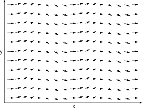
FIG. 1.: Ansatz for the chiral modulation of the molecular tilt in a layer of the smectic-A phase under an applied electric field. The arrows represent the projection of the molecular tilt into the layer plane. The electric field is applied in the $y$ direction, and the average molecular tilt is in the $x$ direction.

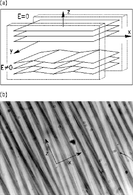
FIG. 2.: (a) Experimental geometry of the striped modulation in the smectic-A phase in narrow cells (from Ref. [14]). (b) Polarization micrograph of the striped pattern in a 15 $\mu$m cell, showing the $xz$ plane (with the line of sight along the $y$ axis). Note that there are two distinct modulations with wavelengths of approximately 30 $\mu$m and 4 $\mu$m, oriented at an angle of approximately 15^∘ with respect to each other (from Ref. [13]).

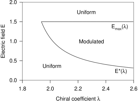
FIG. 3.: Theoretical phase diagram in terms of $\lambda$ and $E$ for fixed $r=0.5$, $u=1$, $b=1$, and $\bar{K}=1.5$, showing the uniform-modulated transitions at $E^{*}(\lambda)$ and $E_{\rm max}(\lambda)$.

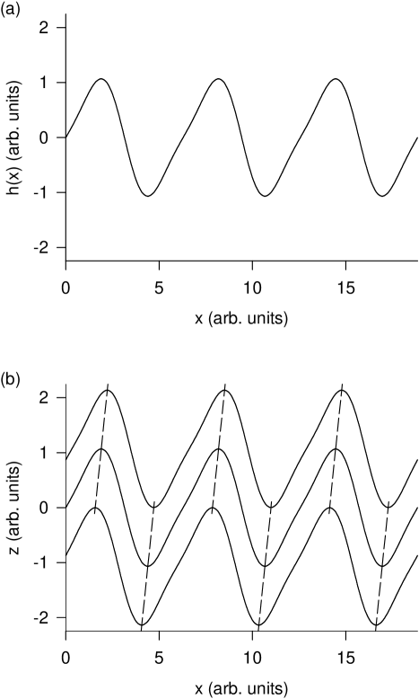
FIG. 4.: (a) Profile of the height modulation of a single smectic layer, showing the $C_{2}^{(y)}$ symmetry. The vertical displacement is highly exaggerated. (b) The most efficient packing of multiple smectic layers with a modulation of this symmetry. The dashed lines indicate the orientation of the stripes in the $xz$ plane.

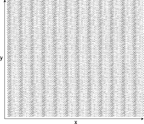
FIG. 5.: Simulation results for the molecular tilt in a layer of the smectic-A phase, showing a chiral modulation for the parameters $r=0.5$, $u=1$, $b=1$, $\bar{K}=1.5$, $\lambda=2.4$, and $E=0.4$. The lines represent the projection of the molecular tilt into the layer plane. The applied electric field is in the $y$ direction.

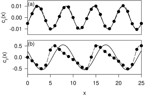
FIG. 6.: Simulation results for the shape of $c_{y}(x)$: (a) Near a transition, for $\lambda=2.25$ and $E=1.48$. (b) Well inside the modulated state, for $\lambda=2.55$ and $E=0.2$. Note that the modulation has a sinusoidal form in the first case, but not in the second.

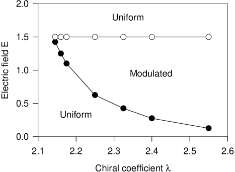
FIG. 7.: Simulation results for the phase diagram in terms of $\lambda$ and $E$ for fixed $r=0.5$, $u=1$, $b=1$, and $\bar{K}=1.5$. The symbols indicate the observed transitions between the uniform and modulated states. The discrepancy between this figure and Fig. 3 is due to the discretization of the lattice.

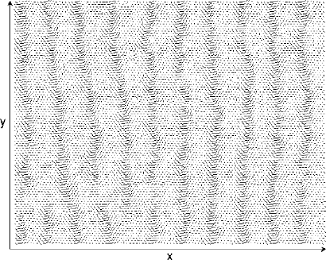
FIG. 8.: Finite-temperature simulation results for the parameters $r=0.5$, $u=1$, $b=1$, $\bar{K}=1.5$, $\lambda=2.4$, and $E=0.2$, showing incipient chiral stripes.

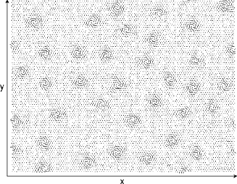
FIG. 9.: Finite-temperature simulation results for the parameters $r=0.5$, $u=1$, $b=1$, $\bar{K}=1.5$, $\lambda=2.4$, and $E=0$, showing localized chiral vortices.

- [1] P. G. de Gennes and J. Prost, The Physics of Liquid Crystals, 2nd ed. (Oxford, 1993).
- [2] S. Garoff and R. B. Meyer, Phys. Rev. Lett. 38, 848 (1977).
- [3] N. A. Clark, D. H. Van Winkle, and C. Muzny (unpublished), cited in Ref. [4].
- [4] S. A. Langer and J. P. Sethna, Phys. Rev. A 34, 5035 (1986).
- [5] G. A. Hinshaw, R. G. Petschek, and R. A. Pelcovits, Phys. Rev. Lett. 60, 1864 (1988).
- [6] G. A. Hinshaw and R. G. Petschek, Phys. Rev. A 39, 5914 (1989).
- [7] A. E. Jacobs, G. Goldner, and D. Mukamel, Phys. Rev. A 45, 5783 (1992).
- [8] Ch. Bahr and G. Heppke, Phys. Rev. A 39, 5459 (1989).
- [9] Ch. Bahr and G. Heppke, Phys. Rev. A 41, 4335 (1990).
- [10] G. P. Crawford, R. E. Geer, J. Naciri, R. Shashidhar, and B. R. Ratna, Appl. Phys. Lett. 65, 2937 (1994).
- [11] A. G. Rappaport, P. A. Williams, B. N. Thomas, N. A. Clark, M. B. Ros, and D. M. Walba, Appl. Phys. Lett. 67, 17 (1995).
- [12] A. Tang and S. Sprunt, Phys. Rev. E 57, 3050 (1998).
- [13] F. J. Bartoli, J. R. Lindle, S. R. Flom, R. Shashidhar, G. Rubin, J. V. Selinger, and B. R. Ratna, Phys. Rev. E 58, 5990 (1998).
- [14] R. E. Geer, S. J. Singer, J. V. Selinger, B. R. Ratna, and R. Shashidhar, Phys. Rev. E 57, 3059 (1998).
- [15] M. S. Spector, S. K. Prasad, B. T. Weslowski, R. D. Kamien, J. V. Selinger, B. R. Ratna, and R. Shashidhar (unpublished).
- [16] T. C. Lubensky, R. D. Kamien, and H. Stark, Mol. Cryst. Liq. Cryst. 288, 15 (1996).
- [17] T. C. Lubensky and F. C. MacKintosh, Phys. Rev. Lett. 71, 1565 (1993).
- [18] C. M. Chen, T. C. Lubensky, and F. C. MacKintosh, Phys. Rev. E 51, 504 (1995).
- [19] C. M. Chen and F. C. MacKintosh, Phys. Rev. E 53, 4933 (1996).
- [20] W. Helfrich and J. Prost, Phys. Rev. A 38, 3065 (1988).
- [21] T. C. Lubensky and H. Stark, Phys. Rev. E 53, 714 (1996).
- [22] J. V. Selinger and R. L. B. Selinger, Phys. Rev. E 51, R860 (1995).
- [23] R. Seidin, D. Mukamel, and D. W. Allender, Phys. Rev. E 56, 1773 (1997).
- [24] G. P. Crawford, J. Naciri, R. Shashidhar, and B. R. Ratna, Jpn. J. Appl. Phys. 35, 2176 (1996).