Noise Stabilization of Self-Organized Memories

Abstract

We investigate a nonlinear dynamical system which “remembers” preselected values of a system parameter. The deterministic version of the system can encode many parameter values during a transient period, but in the limit of long times, almost all of them are forgotten. Here we show that a certain type of stochastic noise can stabilize multiple memories, enabling many parameter values to be encoded permanently. We present analytic results that provide insight both into the memory formation and into the noise-induced memory stabilization. The relevance of our results to experiments on the charge-density wave material $NbSe_{3}$ is discussed.

I Introduction

This paper concerns a nonlinear dynamical system with many degrees of freedom which organizes to store memories, in that a configuration-dependent quantity is driven to take on preselected values. In Ref. [1] it is shown that in the absence of noise, the system encodes many memories during a transient period, but in the limit of long times retains no more than two of them. Thus, the purely deterministic system “learns,” and then it “forgets.”

We examine the effects of adding noise to this system and demonstrate that certain types of noise can stabilize multiple memories so that they are remembered permanently. This noise stabilization is possible because the memory formation mechanism is fundamentally local, whereas forgetting is governed by the large-scale behavior of the system. Thus, it is possible for certain types of stochastic noise to modify the behavior at long wavelengths without destroying the local nonlinear dynamics which give rise to memory creation.

We argue that the type of noise that we have found to stabilize multiple memories is likely to be present in some experiments on charge-density wave (CDW) conductors such as $NbSe_{3}$. Thus, our results could explain the experimental observation of multiple apparently permanent memories encoded in individual samples reported in Ref. [1].

Our analytic investigations of the behavior of this system both with and without noise show that insight into the mechanisms underlying memory formation as well as noise stabilization can be obtained by averaging the dynamical equations over intermediate time periods. We determine analytically the dependence of the memory values on the noise parameters in the limit when a certain parameter $k$ tends to zero. The large-scale behavior of the system follows closely that of a linear diffusion equation; we present analytic bounds on the differences between the evolution of the nonlinear equations and that of the linearized system that are uniform in time and logarithmic in the system size. Some of the analytic results for the system without noise were asserted but not justified in Ref. [1].

The paper is organized as follows. Section II briefly reviews the deterministic version of the model. Sections III and IV present our numerical work demonstrating that noise can stabilize multiple memories. Section V presents our analytic work which enables us to understand why noise can keep memories from being forgotten and also presents an averaging procedure which allows us to obtain analytic insight into the transient memories present in the map without noise in a certain limit. Section VI discusses our main results and possible relevance to CDW experiments. Appendix A demonstrates the uniqueness of the limit obtained by the averaging procedure of section V and also discusses explicitly this limit for the case of multiple memories. Appendix B compares the time evolution of the full nonlinear system with the time evolution of a linearized model and shows that the linearized equations reproduce accurately aspects of the evolution on large scales (though not the memory formation itself).

II The model

First we present the model with no noise, which is the system of coupled maps studied in Ref. [1]:

$$x_{j}(t+1)\ =\ x_{j}(t)+{{\rm f\/loor}}\left[k\sum_{i~{}(nn)}(x_{i}(t)-x_{j}(t))\ -A(t)\right].$$ (1)

Here, $i,j$ are the site indices, the sum is over nearest neighbors, $t$ is a discrete time index, and ${{\rm f\/loor}}[z]$ is the largest integer less than or equal to $z$. This system of maps can be derived from continuous-time differential equations describing the purely dissipative evolution of the positions $x_{j}$ of $N$ particles in a deep periodic potential, with nearest neighbor particles connected by springs of spring constant $k\ll 1$ (see inset, figure 1), in the presence of force impulses $(-A(t)+\frac{1}{2})$[2, 3, 4]. These equations describe the dynamics of sliding charge-density waves (CDW’s),[2, 5, 7], and are closely related to models of a variety of dynamical systems[9]. In this paper we will consider explicitly only one-dimensional systems of $N$ degrees of freedom with one free and one fixed end, $x_{0}(t)=0$ and $x_{N+1}(t)=x_{N}(t)$, starting from the initial condition $x_{j}(t=0)=0$. However, it is straightforward to generalize almost all the results to a variety of different boundary conditions and to more dimensions.

The memory formation that occurs as these maps evolve is manifest in the discrete curvature variables[10]

$$c_{j}(t)\ =\ k\sum_{i~{}(nn)}(x_{i}(t)-x_{j}(t))~{}.$$ (2)

It will be useful to write the dynamical equations in terms of the curvature variables $c_{j}(t)$ rather than the particle positions $x_{j}(t)$. The equations of motion for the $c$’s are:

$$c_{j}(t+1)-c_{j}(t)=$$ (4)

$$k\left\{{{\rm f\/loor}}\left[c_{j+1}(t)-A(t)\right]-2~{}{{\rm f\/loor}}\left[c_{j}(t)-A(t)\right]+{{\rm f\/loor}}\left[c_{j-1}(t)-A(t)\right]\right\}\ ;$$

the fixed chain boundary conditions are[11]

$$c_{0}(t)=A(t)~{},$$ (5)

$$c_{N+1}(t)=c_{N}(t);$$ (6)

and the initial conditions are

$$c_{i}(t=0)=0~{},~{}\ \ \ \mbox{$i\neq 0$}.$$ (7)

Figure 1 shows for these initial conditions the curvature variables $c_{j}(t)$ versus time $t$ for a five-particle chain when $A(t)$ is cycled sequentially through five different values. Memory encoding is manifest by the tendencies of $c$’s to take on values where ${\rm frac}(c)={\rm frac}(A(t))$, where ${\rm frac}(z)=z-{\rm f\/loor}(z)$. That the curvature variables take on values whose fractional part is equal to the fractional part of the force impulse in the maps implies that for the balls and springs, just at the end of each force pulse a significant fraction of the balls are found near the tops of their potential wells[6]. The system “memorizes” the force values and adjusts itself so that the balls are at the well tops just as the pulses end.

As seen in Ref. [1] and here in figure 1, if a repeating sequence of pulses of different lengths is applied, then for a while all the values are encoded. However, at long times the system eventually reaches a fixed point where it stops evolving. At the fixed point, the curvatures are all the same; only one memory is remembered. We have found that using periodic, free, and fixed boundary conditions for the $x$’s, changing the initial conditions, and incorporating quenched (time-independent) randomness to the model do not increase the number of memories retained at the fixed point beyond two.

Here we investigate how this system can be modified so that it can remember more memories permanently. We show that certain types of stochastic noise which are likely to be present in some CDW experiments can do this and study both numerically and analytically the reasons for the multiple-memory stabilization. We show that the stabilization of many memories arises because the noise contains a deterministic component which causes the curvature variables to sustain a large scale spatial variation even in the limit of infinite time. The purely stochastic elements of the noise act to destabilize the memories; we will see that these destabilizing effects vanish in the limit $k\rightarrow 0$.

The following two sections presents our numerical investigations of the model with noise.

III Technique: Adding Noise

Noise terms can be added to Eq. (1) in a variety of ways. Noise which is uncorrelated in both space and time, or uncorrelated in time but spatially uniform (e.g., fluctuations in the pulse amplitudes) does not lead to memory stabilization. However, we have identified a type of noise which is physically plausible that stabilizes multiple memories.

The memory-stabilizing noise we study here is defined by modifying Eq. (1) as follows. Every $\tau$ time steps, an index $j_{D}$ with $1\leq j_{D}\leq N$ is selected, and for all $j>j_{D}$, the positions of balls $j_{D}$ through $N$ are shifted by a fixed integer $X$[8]

$$x_{j}(t+1)=\left\{\begin{array}[]{ll}x_{j}(t)+{\rm f\/loor}[c_{j}(t)-A(t)]+X&\mbox{if $j\geq j_{D}$}\\ x_{j}(t)+{\rm f\/loor}[c_{j}(t)-A(t)]&\mbox{otherwise.}\end{array}\right.$$ (8)

The relative positions of all the balls are unchanged except for the distance between $x_{j_{D}}$ and $x_{j_{D}-1}$, so the disruption is local.

Equivalently, one can write the map with noise in terms of the curvature variables, as

$$c_{j}(t+1)-c_{j}(t) = k\left\{{\rm f\/loor}[c_{j+1}(t)-A(t)]-2~{}{\rm f\/loor}[c_{j}(t)-A(t)]\right.$$ (9)

$$+ \left.{\rm f\/loor}[c_{j-1}(t)-A(t)]\right\}+kX\delta_{t({\rm mod}~{}\tau),0}~{}(\delta_{j,j_{D}-1}-\delta_{j,j_{D}})~{},$$ (10)

where the Kronecker delta $\delta_{i,j}$ is unity if $i$ and $j$ are identical and zero otherwise. In either formulation, the noise does not affect the boundary conditions.

This type of noise models the physical process of breaking the spring connecting balls $j_{D}$ and $j_{D}-1$ and then subsequently reconnecting them with a spring of longer unstretched length[12]. This choice of noise is motivated by phase slip processes known to occur in CDW materials[13]. When the model is applied to CDW’s, the variable $x_{j}$ in Eq. (8) is interpreted as the phase of the charge density wave at the $j^{th}$ impurity site in the sample, measured relative to an undistorted configuration[14, 15, 16]. If a phase slip causes an extra wavelength of the CDW to be inserted between two impurities, then the “unstretched” phase difference between two impurity sites increases.

IV Numerical Results

Fig. 2a shows the behavior of a system identical to that of Fig. 1, except that noise has been applied (Eq. (8)), using the parameter values $X=9$ and $\tau=13$. Fig. 2b shows the time evolution in the presence of noise for a smaller value of $k$. Otherwise the parameters in Fig. 2a and Fig. 2b are identical; in both cases, the index $j_{D}$ in Eq. (8) was selected randomly and with equal probability from the indices $1,...,N$. Fig. 2 demonstrates that when noise is present, more memories are stable at long times than for the noiseless case, Fig. 1. The noise also exhibits a destabilizing effect, as evidenced by the fluctuations in the curvature values. As comparison between Fig. 2a and Fig. 2b demonstrates, these fluctuations become smaller as the parameter $k$ is decreased. Numerically we find that at times $t_{0}$ long enough that the behavior appears to be stationary, the standard deviation of the curvatures from their memory values $\left[\frac{1}{T}\sum_{t=t_{0}+1}^{t_{0}+T}(c_{j}(t)-m_{j})^{2}\right]^{1/2}$ is proportional to $k$ as $k\rightarrow 0$.

Changing the parameters $X$ and $\tau$ can change the number of different stable memories and their values. Below we will show that the memory values attained by each particle in the system can be calculated analytically by averaging the equations of motion of the system.

A Deterministic Noise

In the numerical simulations shown in Fig. 2, the index $j_{D}$ was chosen randomly and with equal probability from the indices $1,\ldots,N$. It is useful to consider a “deterministic” version of noise, where rather than selecting $j_{D}$ randomly, $j_{D}$ is cycled systematically through the indices $1$ to $N$, so that each index is selected exactly once during each noise cycle. (We refer to a “noise cycle” as the $N\tau$ steps it takes to make a complete cycle through the indices $1$ to $N$.) One such choice, used for our numerics, is to cycle through the indices in order, so that

$$x_{j}(t+1)-x_{j}(t)={\rm f\/loor}[c_{j}(t)-A(t)]+X\delta_{t({\rm mod}~{}\tau),0}~{}\theta_{+}(j-\frac{t}{\tau}({\rm mod}~{}N)+1)~{},$$ (11)

where $\theta_{+}(y)=1~{}~{}{\rm if}~{}y\geq 0,$ and zero otherwise. The behavior is substantially identical for any sequence in which each index is chosen exactly once per noise cycle.

Our numerical investigations of the evolution of Eqs. (11) over a wide range of parameters and initial conditions indicate that eventually the system always reaches a periodic orbit. The period of the observed cycle is either equal to or a divisor of $N\tau M$, where again $N$ is the number of balls, $\tau$ is the interval between noise pulses or kicks, and $M$ is the number of memories. Fig. 3 is a plot of the time evolution of the $c_{j}(t)$ for a five-ball system ($N=5$) with the same parameter values as Fig. 2, but with deterministic kicks. The gross features of the curves are very similar, but the fluctuations in the curvature values observed for stochastic noise have been replaced by a regular, repeating pattern (Fig. 4 shows an expanded view of this pattern for two of the $c_{j}$’s). The excursions during the cycles have amplitude proportional to $k$. These regular cycles facilitate analytic investigation of the dependence of stable memories and their values on the parameters $X$ and $\tau$. The number of memories remembered at long times when $k$ is small depends systematically on the ratio $X/\tau$ and not on $X$ and $\tau$ separately. Figure 5 shows numerical results for the dependence of the long-time memory values on $X/\tau$ and demonstrates the good agreement with the analytic predictions presented in the next section.

V Theoretical Analysis

In this section we show how various aspects of the behavior of the maps both with and without noise can be understood analytically in the limit that $k\rightarrow 0$. In subsection (V A) we discuss the map with deterministic noise. The observation that at long times a periodic orbit is always reached can be exploited to predict the dependence of the long-time memory values on the noise parameters $X$ and $\tau$. A key ingredient in this analysis is the examination of the time-averaged equations of motion of the system.

In subsection (V B) we address the model without noise. Because in this case most of the memories are transient and therefore are no longer present when the fixed point is reached, a modified averaging procedure must be used. This procedure yields insight into the transient memories and enables us to demonstrate that a well-defined $k\rightarrow 0$ limit of this model exists.

A Long Time Behavior of The Map with Noise

As Fig. 5 makes evident, there is domain structure to the dependence of the value and number of stable memories on $X/\tau$ for the map with noise, Eqs. (8). Here we calculate analytically the structure of these domains when $k\ll 1$ by finding the memory value of each site as a function of the system parameter $X/\tau$.

The equation of motion for the system is

$$x_{j}(t+1)-x_{j}(t)={\rm f\/loor}[c_{j}(t)-A(t)]+X\theta_{+}(j-j_{D}(t))\delta_{t({\rm mod}~{}\tau),0}~{},$$ (12)

where $\theta_{+}(y)$ is defined after Eq. (11). The $j_{D}$’s are selected so that the probability that $j_{D}(t)=n$ is $P_{n}$. We examine first the case of deterministic noise and discuss stochastic noise at the end of the subsection.

We define an averaging time $T_{ave}=NM\tau$ and

$$\bar{u}_{j}(t_{0})=\frac{1}{T_{ave}}\sum_{t=t_{0}}^{t_{0}+T_{ave}-1}{\rm f\/loor}[c_{j}(t)-A(t)]~{}.$$ (13)

Averaging Eq. (12) over a time $T_{ave}$ yields

$$\frac{1}{T_{ave}}\left(x_{j}(t_{0}+T_{ave})-x_{j}(t_{0})\right)=\bar{u}_{j}(t_{0})+\sum_{n=1}^{j}P_{n}\frac{X}{\tau}~{}.$$ (14)

When $t_{0}$ is large enough so that $x_{j}(t_{0}+T_{ave})=x_{j}(t_{0})$ for all $j$, Eq. (14) implies that the $\bar{u}_{j}(t_{0})$ are independent of $t_{0}$ (hence we drop the argument) and must satisfy

$$\bar{u}_{j}=-\frac{X}{\tau}\sum_{n=1}^{j}P_{n}~{}.$$ (15)

One can also derive Eq. (15) directly in terms of the curvature variables $c_{j}(t)=k(x_{j+1}(t)-2x_{j}(t)+x_{j-1}(t))$. Averaging Eqs. (9) over a time interval $T_{ave}$ yields

$$\frac{1}{T_{ave}}\left[c_{j}(t_{0}+T_{ave})-c_{j}(t_{0})\right] = \bar{u}_{j+1}(t_{0})-2\bar{u}_{j}(t_{0})+\bar{u}_{j-1}(t_{0})+(P_{j+1}-P_{j})\frac{X}{\tau},~{}~{}~{}{j\neq N},$$ (16)

$$= \bar{u}_{j+1}(t_{0})-2\bar{u}_{j}(t_{0})+\bar{u}_{j-1}(t_{0})-P_{N}\frac{X}{\tau},~{}~{}~{}~{}~{}~{}~{}~{}~{}~{}~{}~{}~{}~{}{j=N}.$$ (17)

If $\frac{1}{T_{ave}}\left[c_{j}(t_{0}+MN\tau)-c_{j}(t_{0})\right]=0$, as is true for a periodic orbit, one has

$$\bar{u}_{N}-\bar{u}_{N-1}=-P_{N}X/\tau~{},$$ (18)

$$\bar{u}_{j+1}-\bar{u}_{j}+P_{j+1}{X}/{\tau}=\bar{u}_{j}-\bar{u}_{j-1}+P_{j}{X}/{\tau}~{}~{}~{}~{}(1\leq j<N)~{}.$$ (19)

Eq. (19) implies that $\bar{u}_{j}-\bar{u}_{j-1}+P_{j}X/\tau$ is independent of $j$, which together with the boundary conditions again yields $\bar{u}_{j}=-\frac{X}{\tau}\sum_{n=1}^{j}P_{n}$.

For simplicity, assume that none of the $A_{m}$ are exactly an integer[17] and label the values of $A_{m}$ such that $0<{\rm frac}(A_{1})<{\rm frac}(A_{2})<\ldots<{\rm frac}(A_{M})<1$. We now show that when $k\rightarrow 0$, every particle is almost always on a memory. Only for a set of $P_{n}$ of measure zero are some particles in the system not on memory values as $k\rightarrow 0$. At long times, the $j^{th}$ curvature is on the ${\ell_{j}^{*}}^{th}$ memory ($c_{j}(t\rightarrow\infty)$ obeys ${\rm frac}[c_{j}(t\rightarrow\infty)]={\rm frac}[A_{\ell_{j}^{*}}]+{\mathcal{O}}(k)$), where the memory index $\ell_{j}^{*}$ is

$$\ell_{j}^{*} = 1+{\rm f\/loor}\left[-M\frac{X}{\tau}\sum_{n=1}^{j}P_{n}\right]+\sum_{m=1}^{M}{\rm f\/loor}\left[A_{m}\right]$$ (20)

$$- M\,{\rm f\/loor}\left[-\frac{X}{\tau}\sum_{n=1}^{j}P_{n}+\frac{1}{M}\sum_{m=1}^{M}{\rm f\/loor}\left[A_{m}\right]\right]~{}.$$ (21)

Perhaps surprisingly, which ball is on which memory does not depend on the memory values ${\rm frac}(A_{m})$. This analytic prediction is completely consistent with our numerical observations; this agreement is illustrated by the consistency of the analytic and numerical results presented in figure 5.

We derive Eq. (21) by writing $c_{j}(t)={\mathcal{C}}_{j}+\delta c_{j}(t)$, where each ${\mathcal{C}}_{j}$ is an integer independent of $t$, and $\delta c_{j}(t)$ obeys $0<\delta c_{j}(t)\leq 1$ for all $t$. This decomposition can always be done if $k$ is small enough because the maximum excursion of each $c_{j}$ during the averaging interval is proportional to $k$, and every $c_{j}$ will turn out to be on a memory and hence not at an integer. We define $\delta A_{m}=A_{m}-{\rm f\/loor}(A_{m})$ and

$$\delta\bar{u}_{jm}=\frac{1}{N\tau}\sum_{t=t_{0}}^{t_{0}+T_{ave}-1}\left({\rm f\/loor}[\delta c_{j}(t)-\delta A(t)]\right)\delta_{A(t),A_{m}}~{},$$ (22)

and rewrite Eq. (15) as

$$-\frac{X}{\tau}\sum_{n=1}^{j}P_{n}={\mathcal{C}}_{j}-\frac{1}{M}\sum_{m=1}^{M}{\rm f\/loor}(A_{m})+\frac{1}{M}\sum_{m=1}^{M}\delta\bar{u}_{jm}~{}.$$ (23)

Now $\delta\bar{u}_{jm}=-1$ if $\delta c_{j}(t)<\delta A_{m}$ and $\delta\bar{u}_{jm}=0$ if $\delta c_{j}(t)>\delta A_{m}$ for all $t$ during the averaging interval. Since the excursions during this interval are proportional to $k$, they vanish as $k\rightarrow 0$; thus when $k$ is small enough the $j^{th}$ ball cannot cross more than one memory value during a cycle. Therefore, we can write $\sum_{m=1}^{M}\delta\bar{u}_{jm}=-1+Q_{j}+\rho_{j}$, where $Q_{j}$ is an integer satisfying $0\leq Q_{j}\leq m-1$, and the $\rho_{j}$ satisfy $0<\rho_{j}\leq 1$. Thus we have

$$-\frac{X}{\tau}\sum_{n=1}^{j}P_{n}+\frac{1}{M}\sum_{m=1}^{M}{\rm f\/loor}(A_{m})+1={\mathcal{C}}_{j}+\frac{1}{M}(Q_{j}+\rho_{j})~{},$$ (24)

with ${\mathcal{C}}_{j}$ and $Q_{j}$ integers.

For simplicity we assume here that $MX/\tau\sum_{n=1}^{j}P_{n}$ is not an integer for any $j\leq N$, a condition which will ensure that $\rho_{j}<1$, and hence $\frac{1}{M}(Q_{j}+\rho_{j})<1$[18]. Taking the ${\rm f\/loor}$ of both sides of Eq. (24) yields

$${\mathcal{C}}_{j}={\rm f\/loor}\left[-\frac{X}{\tau}\sum_{n=1}^{j}P_{n}+\frac{1}{M}\sum_{m=1}^{M}{\rm f\/loor}(A_{m})\right]+1~{}.$$ (25)

Multiplying Eq. (24) by $M$ and then taking the ${\rm f\/loor}$ of both sides yields

$$Q_{j} = {\rm f\/loor}\left[-M\frac{X}{\tau}\sum_{n=1}^{j}P_{n}\right]+\sum_{m=1}^{M}{\rm f\/loor}\left[A_{m}\right]$$ (26)

$$- M\,{\rm f\/loor}\left[-\frac{X}{\tau}\sum_{n=1}^{j}P_{n}+\frac{1}{M}\sum_{m=1}^{M}{\rm f\/loor}\left[A_{m}\right]\right],$$ (27)

which in turn implies

$$\rho_{j}=-M\frac{X}{\tau}\sum_{n=1}^{j}P_{n}-{\rm f\/loor}\left[-M\frac{X}{\tau}\sum_{n=1}^{j}P_{n}\right]~{}.$$ (28)

We see that it is consistent to assume that $0<\rho_{j}<1$ so long as $(MX/\tau)\sum_{n=1}^{j}P_{n}$ is not exactly an integer. Since $\rho_{j}$ can only be fractional if $c_{j}$ crosses a memory during the averaging interval, as $k\rightarrow 0$ each $c_{j}$ must be on a memory. Since $Q_{j}$ determines the memory index via $\ell_{j}^{*}=Q_{j}+1$, one obtains Eq. (21).

Finally, to demonstrate consistency of the assumption that no particle can be on more than one memory, we must show that the particle excursions over the averaging time are small as $k\rightarrow 0$. This is easily done starting from the equation of motion for the curvatures Eq. (9) and noting that our solution for the $\bar{u}_{j}$ satisfies $\bar{u}_{j+1}-2\bar{u}_{j}+\bar{u}_{j-1}=0$. If no memory is crossed, then the absolute value of the difference between the time average $\frac{1}{T_{ave}}\sum_{t_{0}}^{t_{0}+T_{ave}}{\rm f\/loor}[{c}_{j}(t)-A(t)]\delta_{A(t),A_{m}}$ and the corresponding ${\rm f\/loor}[c_{j}(t)-A(t)]\delta_{A(t),A_{m}}$ cannot be bigger than unity. This bound implies that until a memory is crossed, the excursion per unit time of each of the $c$’s cannot be bigger than $k(4+X)$. Since the memory values are separated by an amount of order unity, as $k\rightarrow 0$ the number of steps needed to reach the nearest memory diverges as $1/k$, and the excursion during the averaging time cannot be greater than $k(4+X)T_{ave}$.

1 Importance of Spatial Distribution of the Noise

So far we have mainly discussed the case of spatially homogeneous noise, $P_{n}=1/N$ for all $n$, and seen that if the noise causes each spring in the chain to break with equal probability, multiple memories can be stabilized indefinitely. However, in our analytic work we did not assume this special form for $P_{n}$, and one may ask whether the same results are obtained if, for instance, only the first spring were broken repeatedly.

We address this issue by examining Eq. (21). Note that if $P_{l}=0$ for some $l$, then particles $l-1$ and $l$ must be on the same memory value. Thus, if only the first spring is repeatedly broken, there will be only one memory observed at long times, although its value may be different than in the noiseless case. However, the $P_{n}$ need not all be equal for multiple memories to be stable at long times.

2 Stochastic Versus Deterministic Noise

Now we discuss the behavior when the system is subject to stochastic noise rather than deterministic noise. The crucial point here is that the equations of motion can always be averaged over some time interval $T_{ave}$, and so long as all the $c_{j}$’s stay roughly constant, there is no need for there to be a truly periodic cycle for the procedure above to apply. As $k\rightarrow 0$ the memory values will be exactly the same for random noise as for deterministic kicks with the same time-averaged spatial distribution of events.

Not surprisingly, the excursions of the curvatures about the memory values are larger for stochastic noise than for sequential kicks, all other parameters being held fixed. There are two mechanisms by which stochastic noise would enhance the size of the excursions. The first is that the small motions of the curvatures about their memory values are more erratic because the noise kicks are inhomogeneously spaced in time, and the second is that fluctuations in the noise may temporarily cause the system to be driven to a memory value other than that determined by the time-averaged $X/\tau$. Numerically we find that the excursions in systems with stochastic noise are typically a few times the excursions observed in the deterministic case with the same parameters, and that their magnitude is proportional to $k$. These observations are evidence that the first mechanism is dominant; the second mechanism leads to a nonlinear dependence of the excursions on $k$ and also, since it depends on how far each curvature is from the edge of the parameter range in which the memory in question is stable, leads to sensitive dependence of the excursion magnitudes on $X$ and $\tau$.

B The behavior of the map without noise as $k\rightarrow 0$

In this subsection we show that a modified averaging procedure can be used to obtain insight into the time evolution of the system.

Above, we used the observation that at long times the behavior of the map with noise is periodic in time to calculate how the memory values depend on the system parameters. A key step in this calculation is averaging the equations of motion of the system over an appropriate time interval. Here we present an averaging procedure applicable in the limit $k\rightarrow 0$ that can be used to obtain insight into the time evolution and not just the long time behavior.

Analyzing just the long-time behavior cannot yield insight into transient memories, because in this limit almost all the memories have been forgotten. Therefore, the technique we used in the previous subsection of looking only at fixed points of the equations of motion is not so useful here. However, Fig. 6, which shows the evolution of the curvatures for the system with no noise (the same numerical data as Fig. 1 on an expanded scale), demonstrates that during the motion two types of particles exist—sites whose curvatures are “stuck” on a memory values, and curvatures that are in transit between different memory values (“drifting”). A “stuck” site oscillates periodically about a memory value until a neighbor changes its status, at which time the stuck site can either change its oscillation about the same memory, or can start to drift. As $k$ is decreased, it takes more and more time steps for the drifting sites to get between different memories, during which time they provide a constant environment for their neighbors. In contrast, the period of the cycles of the “stuck” sites remains unchanged as $k\rightarrow 0$; moreover, the amplitudes of the excursions about the memory values are proportional to $k$. In the limit $k\rightarrow 0$, the drifting sites comprise a quasi-stationary environment for the stuck sites, and one can average the equations of motion over the period of the stuck sites’ cycles.

For simplicity, in this subsection we consider only the case of a single memory with $A=0$. The generalization of the analysis to different memory values and to multiple memories is straightforward, and is discussed briefly in Appendix A. We only discuss here the model in the absence of noise, but the analysis is easily extended to the case when noise is present, if desired.

The equations of motion for the $c_{j}(t)$ are

$$c_{j}(t+1)=c_{j}(t)+k\left({\rm f\/loor}[c_{j+1}(t)]-2\,{\rm f\/loor}[c_{j}(t)]+{\rm f\/loor}[c_{j-1}(t)]\right)~{}.$$ (29)

First consider the behavior of a site $j$ whose two neighbors’ curvatures are both drifting between integers. While the sites $j+1$ and $j-1$ are drifting, the quantities ${\rm f\/loor}[c_{j+1}(t)]$ and ${\rm f\/loor}[c_{j-1}(t)]$ remain constant, and we can denote their (integer) values as $I_{j+1}$ and $I_{j-1}$ and define $\eta\equiv(I_{j+1}+I_{j-1})/2$. Eq. (29) then becomes

$$c_{j}(t+1)-c_{j}(t)=2k\left(\eta-{\rm f\/loor}[c_{j}(t)]\right)~{}.$$ (30)

If $\eta-{\rm f\/loor}[c_{j}(t)]>0$, then $c_{j}(t)$ will increase in time until $\eta-{\rm f\/loor}[c_{j}(t)]$ is no longer positive. If $\eta$ is an integer, then $c_{j}(t)$ will stick at $\eta$, whereas if $\eta$ is a half-integer, then $c_{j}(t)$ will undergo a period-2 cycle about the integer value $\eta+1/2$. If initially $\eta-{\rm f\/loor}(c_{j}(t))<0$, then eventually $c_{j}(t)$ will stick just below $\eta+1$ if $\eta$ is an integer, and $c_{j}(t)$ will oscillate in a period-2 cycle cycle about $\eta+1/2$ if $\eta$ is a half-integer.

If there are $L$ stuck sites in a row, then the cycles of the sites become longer, but simple periodic behavior is still observed. We find numerically that the motion of each site in a stuck region with $L$ sites is a cycle of length $L+1$ or shorter. Moreover, every time a site changes its status (for instance, a drifting site might come within $O(k)$ of a memory value), the new cycle gets established in a time that remains finite as $k\rightarrow 0$. Therefore, as $k\rightarrow 0$, during the periods when the drifting sites at the boundaries of the region in question remain between memories, we can average Eqs. (29) over the cycle of length $p$. Defining $u_{j}=\frac{1}{p}\sum_{t=t_{0}+1}^{t_{0}+p}{\rm f\/loor}[c_{j}(t)]$, we obtain

$$c_{j}(t+p)-c_{j}(t)=k\left(u_{j+1}-2u_{j}+u_{j-1}\right)~{}.$$ (31)

All the terms on the right hand side of Eq. (31) are time-independent, implying that

$$c_{j}(t_{0}+p)=c_{j}(t_{0})+(kp)r_{j}~{},$$ (32)

with $r_{j}=u_{j+1}-2u_{j}+u_{j-1}$. Moreover, we can rewrite Eq. (29) during the averaging interval as

$$c_{j}(t+1)=c_{j}(t)+kr_{j}+k\Delta_{j}(t)~{},$$ (33)

where $\Delta_{j}(t)={\rm f\/loor}[c_{j+1}(t)]-u_{j+1}-2({\rm f\/loor}[c_{j}(t)]-u_{j})+{\rm f\/loor}[c_{j-1}(t)]-u_{j-1}$ has zero mean and is periodic with period $p$. Also, because ${\rm f\/loor}(c_{j})$ of a stuck site does not change by more than $\pm 1$, we have $|\Delta_{j}(t)|<4$. Therefore, we can write the complete solution of Eq. (29) for the interval where all the stuck sites have settled into their periodic behavior and none of the drifting sites goes through an integer as

$$c_{j}(t_{0}+l)=c_{j}(t_{0})+(kl)r_{j}+k\eta_{j}(l)~{},$$ (34)

where $\eta_{j}(l)$ is periodic in time and satisfies $|\eta_{j}(l)|<4\max\{p_{j}\}<4N$ for all $j$ and $l$. The first two terms represent the piecewise linear solution and the last term represents the cycles of amplitude of order $k$ superimposed on the piecewise linear solution. Note that the difference between the piecewise linear part of the solution and the complete solution goes to zero as $k\rightarrow 0$.

We can define a rescaled time variable $\tilde{t}=k*t$ and take the limit of Eq. (34) with $k\rightarrow 0$, $kl$ finite, in which the $u_{j}$ (and hence $r_{j}$) are independent of $k$. The existence and uniqueness of this limit is demonstrated in Appendix A. In this limit, the solution converges to

$$c_{j}(\tilde{t_{0}}+\tilde{t})=c_{i}(\tilde{t_{0}})+r_{i}\tilde{t}.$$ (35)

If a site $j$ is drifting, we set $u_{j}={\rm f\/loor}(c_{j})$, whereas if it is stuck, $u_{j}$ is determined by requiring

$$r_{j}=u_{j+1}-2u_{j}+u_{j-1}=0~{}.$$ (36)

When there are $L$ stuck sites in a row (say sites $u_{j_{0}+1},\ldots,u_{j_{0}+L}$, with $u_{j_{0}}$ and $u_{j_{0}+L+1}$ given), then the $u_{j}$ in the stuck region are obtained by solving Eq. (36), yielding

$$u_{j}=u_{j_{0}}+\left(\frac{u_{j_{0}+L+1}-u_{j_{0}}}{L+1}\right)(j-j_{0})~{}.$$ (37)

Whenever all the $u_{j}$ are fractional, every site in the region must be on a memory. The values of $u_{j_{0}+1}$ and $u_{j_{0}+L}$ enter into the drift rates of $c_{j_{0}}$ and $c_{j_{0}+L+1}$ and hence must be determined to obtain the time evolution of those sites.

One still needs to consider the behavior at the transitions when the sites change between stuck and drifting. Because the number of steps needed to establish the new cycle structure is finite and independent of $k$, these transitions are instantaneous in terms of rescaled time. Moreover, as we demonstrate in Appendix A, the values of the $u$’s after each transition do not depend on the details of either the old cycle structure or of the transition.

These considerations enable us to use the the piecewise linear solution Eq. (35) to formulate a $k=0$ model. In the $k=0$ model, if a site $i$ is stuck, then $c_{i}$ is exactly an integer. Between transitions,

$$\frac{dc_{j}}{dt}=u_{j+1}-2u_{j}+u_{j-1}~{},$$ (38)

where the $u_{j}$ are equal to the $u_{j}$ that are defined for a system with non-zero $k$ by averaging between the same two transitions. At each transition, the $c_{j}$ are continuous. However, the $u_{j}$ change instantaneously to the new values appropriate to the time interval after the transition but before the next transition.

Thus we have been able to characterize the local dynamics, and describe the $k\rightarrow 0$ limit of the model. However, we have not addressed the evolution of the large scale structure of the system. Ref. [1] presents numerical evidence that all the large-scale structure of the nonlinear equations is well-approximated by the evolution of linear equations of motion obtained by replacing ${\rm f\/loor}[y]$ by $y-\frac{1}{2}$ in Eq. (4). As discussed in Ref. [1], this observation enables one to perform accurate estimates of when memories form and when they are forgotten as a function of system size and model parameters. In Appendix B we present an analytic bound on the error in the evolution of the curvatures made when the dynamical equations are linearized and show that this error is bounded uniformly in time and logarithmically in the system size.

In this subsection we have obtained the $k\rightarrow 0$ behavior via an explicit limiting process of the dynamics with $k\neq 0$. In Appendix A we show that this limit is well-defined and prescribe how to define the $k\rightarrow 0$ limit of the model without reference to averages of the $k\neq 0$ dynamics. We also sketch how to generalize the analysis of the $k\rightarrow 0$ limit to apply to the case of multiple memories.

VI Discussion

We have investigated the behavior of a simple nonlinear dynamical system which has the capacity to encode memories. The deterministic system can encode many memories for a while, but at long times forgets almost all of them. Here we have demonstrated that there is a type of stochastic noise which enables the system to encode many memories permanently. The memory stabilization arises because the noise has a time-average with nontrivial spatial structure; in particular, it enables the curvature variables which describe the local force, to have large-scale variations even at long times.

The disappearance of the memories in the absence of noise occurs only because the range of $c$’s collapses at long times. For fixed, free, or periodic boundary conditions (which seem most appropriate to physical realizations of balls and springs or of charge-density waves), at long times the values of $c_{0}$ and $c_{N}$ are the same. To stabilize many memories permanently, one must arrange things so that $c_{0}\neq c_{N}$ at long times. The “phase slip” noise studied here is one way to do this. In principle, another way to do this is to impose boundary conditions which enforce $c_{0}\neq c_{N}$, but we do not know of a physically plausible way to do this in the CDW system[19].

We now discuss possible consequences of our results for experiments on CDW materials. The experiments reported in Ref. [1] involved averaging over millions of applied pulses, and thus were probably measuring the number of memories retained in steady-state[1]. In the experiment, the only samples which retained multiple memories had additional silver paint strips attached between the probe contacts. This perturbation on the system is important, because ordinarily one expects the phase slips to occur almost exclusively at the sample contacts, where the strains are largest[13]. The silver paint in the middle of the sample may induce spatially inhomogeneous phase slips; our theoretical results suggest that the spatial inhomogeneity of phase slips in a sample may be important in determining the number of memories retained at long times. Further experiments to quantify the spatial dependence of noise in CDW materials would help determine whether the theory is applicable to noise production in this experimental situation.

Because the noise stabilization depends on the detailed spatial characteristics of the noise, it will be quite sample-dependent. On the other hand, in the absence of noise, the dependence of the duration of the transient memories on sample size follows from rather general arguments and should be robust[1]. Therefore, systematic investigation of the time evolution of the transient memory response in samples with as little noise as possible is therefore probably the most promising avenue towards making comparison between theory and experiment.

In this paper we have shown that it is possible to obtain a rather complete theoretical understanding of our dynamical system in the limit of very weak springs, $k\rightarrow 0$. However, real CDW materials such as $NbSe_{3}$ tend to be described by the model in the large-$k$ regime[20]. Therefore, quantitative comparison between this theory and experiment cannot be expected. Understanding how the memory behavior evolves as $k$ is made large and providing quantitative theoretical predictions in the regime relevant to experiment is an important subject for future investigations.

VII Acknowledgments

S.N.C. acknowledges support by the National Science Foundation, Award No. DMR 96-26119. L.P.K. acknowledges support from the Office of Naval Research, Grant N00014-96-1-0127. M.L.P. acknowledges support through the NSF Materials Research Science and Engineering Center summer REU program. This work was supported in part by the MRSEC program of the National Science Foundation under Award Nos. DMR-9400379 and DMR-9808595.

Appendix A: The ${\mbox{\boldmath$k$}}\rightarrow 0$ limit

In Subsection (V B) we defined the $k\rightarrow 0$ limit of the model in terms of averages of the behavior of the model with nonzero $k$. In this appendix, we demonstrate that this limit is well-defined and show how to construct it without reference to the system with nonzero $k$. In A.I we discuss a single integer memory, while in A.II we consider briefly the rather straightforward generalization to the case of multiple memories.

A.I: The $k=0$ limit

We recall that our original model was defined in terms of a discrete time index $t$, and wish to introduce a rescaled time $\tilde{t}=kt$ and consider the limit $k\rightarrow 0$ with $\tilde{t}$ finite. The problem we are addressing is: Given values $c_{j}(\tilde{t})$ for $j=1,2,\ldots,N$ at some time $t$, can the corresponding $u_{j}(\tilde{t})$ be generated uniquely? If so, then because $\frac{dc_{j}}{d\tilde{t}}=u_{j+1}(\tilde{t})-2u_{j}(\tilde{t})+u_{j-1}(\tilde{t})$, the entire time evolution is determined.

As stated, this problem is not solvable in general. This is because, even for a model with non-zero $k$, the $u_{j}$ are not defined uniquely at a “transition” at which the sites go from one distribution of “stuck” sites or a given cycle structure to another. As an illustration, consider the system

$$c_{1}(t+1)=c_{1}(t)-k(u_{0}+u_{2}-2{\rm f\/loor}[c_{1}(t)])~{},$$ (39)

where $u_{0}=0$ and $u_{2}=1$. If initially $c_{1}(0)=1+7k/2$, we have $c_{1}(t)=1+(7-2t)k/t$, $t\leq 4$ and $c_{1}(t)=1-(-1)^{t}k/2$, $t>4$. On the other hand, if initially $c_{1}(0)=1-7k/2$, then $c_{1}(t)=1-(7-2t)k/t$, $t\leq 4$ and $c_{1}(t)=1+(-1)^{t}k/2$, $t>4$. Therefore, for $t\leq 4$, the two different initial conditions yield $u_{1}(0)=1$ and $u_{1}(0)=0$, respectively. As $k\rightarrow 0$, both these situations correspond to the same initial condition $c_{1}(0)=1$, and therefore it is clear that there is a transient period when $u_{1}(0)$ is not defined uniquely. Nonetheless, since both initial conditions in the example yield $u_{1}(\tilde{t})=1/2$ for $\tilde{t}>4k$, in the limit $k=0$ it is consistent to define $u_{1}(\tilde{t})=1/2$ for all $\tilde{t}>0$.

Here we demonstrate that $u_{1}(\tilde{t})$ for $\tilde{t}>0$ can be defined uniquely for all possible initial conditions of the model with non-zero $k$ that lead to the same initial configuration of $c$’s as $k\rightarrow 0$. Specifically, we show that given values $c_{j}(\tilde{t_{0}})$ for $j=1,2,\ldots,N$ there is a unique consistent way to define $u_{j}(\tilde{t})$ for $\tilde{t}$ such that $\tilde{t}>\tilde{t_{0}}$, valid up until the next transition. This fact, together with the observation that the functions $c_{j}(t)$ are continuous, enables us to show that the $k=0$ limit of our model is well-defined.

For the $k\neq 0$ model, we have that $u_{j}={\rm f\/loor}(c_{j})$ unless $c_{j}$ is within $O(k)$ of an integer $m$. If we are close to a transition, we cannot define the $u_{j}$’s for all the sites that are close to integers. However, recall that each transition takes a finite number of steps, and hence takes up zero units of the rescaled time $\tilde{t}=kt$ as $k\rightarrow 0$. The $c_{j}$ change in steps of $O(k)$, so the sites where $c_{j}$ is initially close to an integer will have a $c_{j}$ that is close to the same integer after the transition. After the transition, we have one of the following possibilities for these sites:

1. The site $j$ could be stuck (more precisely, the curvature of site $j$ could be stuck) and the value of $c_{j}$ will execute a cycle (possibly of period 1) near the integer. In this case, we have $m-1\leq u_{j}\leq m$ and the site has zero average drift.

2. The site could be drifting up on average. In this case, $c_{j}>m$ after the transition so that $u_{j}=m$.

3. The site $j$ could be drifting down on average. In this case $c_{j}<m$ after the transition so that $u_{j}=m-1$.

Since we have that the average drift rate for the site $j$ after the transition is given by

$$\frac{dc_{j}}{d\tilde{t}}=u_{j+1}(\tilde{t})-2u_{j}(\tilde{t})+u_{j-1}(\tilde{t}),$$ (40)

we have the following consistency conditions:

$$u_{j}(\tilde{t})>m-1\mbox{ implies that }u_{j+1}(\tilde{t})-2u_{j}(\tilde{t})+u_{j-1}(\tilde{t})\geq 0~{},$$ (41)

$$u_{j}(\tilde{t})<m\mbox{ implies that }u_{j+1}(\tilde{t})-2u_{j}(\tilde{t})+u_{j-1}(\tilde{t})\leq 0~{}.$$ (42)

These conditions are independent of $k$, and we require that the $k=0$ model satisfy them. In the $k=0$ model, a site can be stuck only if $c_{j}$ is exactly an integer. If $c_{j}$ is not exactly an integer, then since $c_{j}(t)$ is continuous, we have

$$u_{j}(\tilde{t}_{0+})={\rm f\/loor}[c_{j}(\tilde{t_{0}})]~{},$$ (43)

where $\tilde{t}_{0+}=\lim_{\epsilon\rightarrow 0+}u(\tilde{t_{0}}+\epsilon)$. If $c_{j}(\tilde{t_{0}})=a$ is exactly an integer, we have that

$$a-1\leq u_{j}(\tilde{t}_{0+})\leq a.$$

We can combine the preceding two equations to obtain

$$u^{-}(c_{j})\leq u_{j}\leq u^{+}(c_{j}),$$ (44)

where $u^{-}(x)=\lim_{\epsilon\rightarrow 0+}{\rm f\/loor}(x-\epsilon)$ and $u^{+}(x)=\lim_{\epsilon\rightarrow 0+}{\rm f\/loor}(x+\epsilon)$. The functions $u^{+}$ and $u^{-}$ satisfy a monotonicity condition

$$u^{-}(a)\leq u^{+}(a)\leq u^{-}(b)\leq u^{+}(b)$$ (45)

for all $a<b$ (this follows from the fact that ${\rm f\/loor}(x)<{\rm f\/loor}(y)$ if $x<y$). This implies that for any given value $u$, there is at most one value of $c$ such that it is possible for a site with $c_{j}=c$ to have $u_{j}=u$. This monotonicity gives the following consistency requirement on the definition of the $u_{j}(\tilde{t}_{0+})$:

$$u_{j}(\tilde{t}_{0+})>u^{-}(c_{j}(\tilde{t_{0}}))\mbox{ implies that }u_{j+1}(\tilde{t}_{0+})-2u_{j}(\tilde{t}_{0+})+u_{j-1}(\tilde{t}_{0+})\geq 0~{},$$ (46)

$$u_{j}(\tilde{t}_{0+})<u^{+}(c_{j}(\tilde{t_{0}}))\mbox{ implies that }u_{j+1}(\tilde{t}_{0+})-2u_{j}(\tilde{t}_{0+})+u_{j-1}(\tilde{t}_{0+})\leq 0~{}.$$ (47)

For brevity, we will henceforth suppress the time arguments; $c_{j}$ will represent $c_{j}(\tilde{t_{0}})$ and $u_{j}$ will represent $u_{j}(\tilde{t}_{0+})$.

We are trying to generate the $u_{j}$ given the $c_{j}$ so that the $k=0$ model is well defined. Given the $c_{j}$, we can take an initial condition of the form $\tilde{c}_{j}=c_{j}+kF_{j}$, where the $F_{j}$ is a given arbitrary bounded sequence, and choose $k$ sufficiently small so that $\tilde{c}_{j}$ is not an integer if $c_{j}$ is not an integer and $|\tilde{c}_{j}-c_{j}|\leq 1/4$ for all $j$. Then the $u_{j}$ obtained by following the dynamics in a model with finite $k$ starting from this initial condition and looking at the averages after any initial transitions will satisfy the consistency requirements. However, it is not clear that this procedure gives a unique definition of $u_{j}$.

To show that there is only one consistent way to define $u_{j}$ for a given $c_{j}$, we assume the opposite. Let $u^{1}_{j}$ and $u^{2}_{j}$ be two distinct definitions for $u_{j}$ that are both consistent. Both $u^{1}_{j}$ and $u^{2}_{j}$ satisfy the same boundary conditions, so that $u^{1}_{0}-u^{2}_{0}=0$ and $u^{1}_{N}-u^{2}_{N}=0$. Since $u^{1}\neq u^{2}$, there is some index $j^{*}$ for which $u^{1}_{j^{*}}-u^{2}_{j^{*}}\neq 0$. Without loss of generality, we choose the labels so that $u^{1}_{j^{*}}-u^{2}_{j^{*}}>0$. Since $u^{1}_{0}-u^{2}_{0}=0$ and $u^{1}_{N}-u^{2}_{N}=0$, there must exist indices $p$ and $q$ with $p<j^{*}<q$ such that $u^{1}_{p}-u^{2}_{p}\leq 0$, $u^{1}_{q}-u^{2}_{q}\leq 0$, and $u^{1}_{j}-u^{2}_{j}>0$ for all $p<j<q$. By Eq. (44), $u^{2}_{j}\geq u^{-}(c_{j})$, so that $u^{1}_{j}>u^{-}(c_{j})$ for all $p<j<q$. Eq. (47) therefore requires that $u^{1}_{j+1}+u^{1}_{j-1}-2u^{1}_{j}\geq 0$ for all $p<j<q$. Eq. (44) also implies that $u^{1}_{j}\leq u^{+}(c_{j})$, so that $u^{2}_{j}<u^{+}(c_{j})$ for all $p<j<q$. Eq. (47) therefore requires that $u^{2}_{j+1}+u^{2}_{j-1}-2u^{2}_{j}\geq 0$ for all $p<j<q$. Combining these two results, we have

$$(u^{1}_{j+1}-u^{2}_{j+1})+(u^{1}_{j-1}-u^{2}_{j-1})-2(u^{1}_{j}-u^{2}_{j})\geq 0$$

for all $p<j<q$. This implies that if $u^{1}_{j}-u^{2}_{j}$ attains a maximum on $p<j<q$, it is a constant for $p\leq j\leq q$. Therefore, $u^{1}_{j}-u^{2}_{j}\leq\max(u^{1}_{p}-u^{2}_{p},u^{1}_{q}-u^{2}_{q})=0$ for all $p<j<q$. This contradicts our assumption that $u^{1}_{j^{*}}-u^{2}_{j^{*}}>0$, and proves that there can be only one consistent definition of $u_{j}$ given $c_{j}$. This proves the claim from section V that averaging over the cycles in a $k\neq 0$ model gives a consistent $k=0$ model.

Now we present a prescription for generating the $u_{j}$ from the $c_{j}$ without any reference to the $k\neq 0$ model. The process consists of identifying all sites whose $u$’s must be integers, requiring that all the remaining $u$’s satisfy $u_{j+1}-2u_{j}+u_{j-1}=0$, and checking to see whether all the constraints are satisfied. If not, then there is at least one additional site whose $u$ is an integer, and one such site is identified. This process is iterated until all the constraints are satisfied.

First consider the situation where $u_{0}=u_{p}=0$. We are given a sequence $c_{j}$ ($0<j<p$) and hence functions $u_{i}^{+}(c)$ and $u_{i}^{-}(c)$ that satisfy the monotonicity condition (45) for each $0<i<p$. The dynamics of the $c_{j}$ are determined by Eq. (40), and each $u_{j}$ must satisfy the constraint $u_{j}^{-}(c_{j})\leq u_{j}\leq u^{+}_{j}(c_{j})$. Our earlier results generalize to this case and it follows that there is a unique assignment of the $u_{j}$ that satisfy the consistency conditions in Eq. (47). In this situation we have the following result:

Claim 1: Let $j^{*}$ be an index where $u_{j}^{-}(c_{j})$ attains a maximum for $0<j<p$ and $u_{j^{*}}^{-}(c_{j^{*}})>0$. Then we must have $u_{j^{*}}=u_{j^{*}}^{-}(c_{j^{*}})$.

Proof: Assume that this is not true. Then, we must have $u_{j^{*}}>u_{j^{*}}^{-}(c_{j^{*}})$, and the consistency condition requires that $u_{j^{*}+1}+u_{j^{*}-1}-2u_{j^{*}}\geq 0$. It follows that $u_{j^{*}}$ is not a strict maximum for $u_{j}$ for $0\leq j\leq p$. Let $0<m<p$ be such that $u_{m}\geq u_{j^{*}}$. Since the maximum value for $u_{j}^{-}(c_{j})$ was attained at $j=j^{*}$, it follows that $u_{m}>u^{-}_{m}(c_{m})$. Therefore, by the preceding argument with $m$ in the place of $j^{*}$, it follows that $u_{m}$ is not a strict maximum for $u_{j}$. Consequently, $u_{j}\leq\max(u_{0},u_{p})=0$ for all $0<j<p$. This contradicts the fact that the $u_{j}$ are constrained to be greater than or equal to $u^{-}_{j}(c_{j})$ and $u_{j^{*}}^{-}(c_{j^{*}})>0$.

A similar argument shows that if $j^{*}$ is an index where $u_{j}^{+}(c_{j})$ attains a minimum for $0<j<p$ and $u_{j^{*}}^{+}(c_{j^{*}})<0$, then $u_{j^{*}}=u_{j^{*}}^{+}(c_{j^{*}})$.

If $u_{j}^{-}(c_{j})\leq 0$ and $u_{j}^{+}(c_{j})\geq 0$ for all $0<j<p$, the preceding result does not give us any information. However, in this case we can set $u_{j}=0$ for $0\leq j\leq p$. Since this assignment satisfies the constraint and the consistency conditions, by our earlier result, it is the unique consistent definition for $u_{j}$.

Now we can solve the problem of assigning the $u_{j}$ given the $c_{j}$ for the $k=0$ model recursively. Assume that we know $u_{p}=a$ and $u_{q}=b$ with $p>q$.[26] Let

$$l_{i}=a\frac{q-i}{q-p}+b\frac{i-p}{q-p}.$$

For $p<i<q$ define $\tilde{u}_{i}^{\pm}(c)=u_{i}^{\pm}(c)-l_{i}$ and $\tilde{u}_{i}=u_{i}-l_{i}$. Since $l_{j+1}+l_{j-1}-2l_{j}=0$, it follows that we are precisely in the situation that we considered above.

We set $u_{j}=l_{j}$ for all $p<j<q$ and check to see if $\tilde{u}_{j}^{-}(c_{j})\leq 0$ and $\tilde{u}_{j}^{+}(c_{j})\geq 0$ for all $p<j<q$. If not, we find an index $j^{*}$ and fix $u_{j^{*}}$ as in Claim 1 above, and repeat the procedure for $p<j<j^{*}$ and $j^{*}<j<q$. This determines all the $u_{j}$ recursively in no more than $N$ steps.

The $u_{j}$ determine the time dependence of the $c$’s via $\frac{dc_{j}}{d\tilde{t}}=u_{j+1}-2u_{j}+u_{j-1}$. The complete solution between the transitions at $\tilde{t}=\tilde{t}_{n}$ and $\tilde{t}=\tilde{t}_{n+1}$ is given by

$$c_{j}(\tilde{t})=c_{j}(\tilde{t}_{n})+r_{j}(\tilde{t}-\tilde{t}_{n})\hskip 24.0pt\mbox{for $\tilde{t}_{n}\leq\tilde{t}\leq\tilde{t}_{n+1}$}.$$ (48)

A.II: Multiple Memories

Now we extend our analysis of the $k\rightarrow 0$ limit to the case of multiple memories. We find

$$\frac{dc_{j}}{d\tilde{t}}=U_{j+1}-2U_{j}+U_{j-1}~{},$$ (49)

with the $U_{j}$ given by

$$U_{j}=\frac{1}{p_{j}}\sum_{t=0}^{p_{j}-1}{\rm f\/loor}[c_{j}(t_{0}+t)-A(t_{0}+t)]$$ (50)

if the site $j$ is stuck in a cycle of period $p_{j}$, and

$$U_{j}=\frac{1}{M}\sum_{t=0}^{M-1}{\rm f\/loor}[c_{j}(t_{0}+t)-A(t_{0}+t)]$$ (51)

if the site $j$ is drifting, i.e., the fractional part of $c_{j}$ is not equal to the fractional parts of any of the forcings $A(1),A(2),\ldots,A(M)$. We define

$$U^{-}=\lim_{\epsilon\rightarrow 0+}\frac{1}{M}\sum_{m=0}^{M-1}{\rm f\/loor}[c_{j}-\epsilon-A(m)]$$ (52)

and

$$U^{+}=\lim_{\epsilon\rightarrow 0+}\frac{1}{M}\sum_{m=0}^{M-1}{\rm f\/loor}[c_{j}+\epsilon-A(m)]~{}.$$ (53)

Then we can assign the stuck sites and the drifting sites by the same procedure as for the single memory except that we replace $u^{-}$ by $U^{-}$ and $u^{+}$ by $U^{+}$.

Appendix B: The linearized map

In this appendix, we address the large-scale dynamics of the system by examining a linearized equation obtained by approximating the ${\rm f\/loor}$ function in Eq. (4) with $z-1/2$, yielding the linearized map:

$$c_{j}(t+1)-c_{j}(t)=k\left[c_{j+1}(t)-2c_{j}(t)+c_{j-1}(t)\right]~{}.$$ (54)

Although this linearized map contains no information about the memory formation, it captures accurately the behavior of the system at large scales. Ref. [1] presented numerical evidence for this observation, and showed that it enables one to obtain analytic estimates on the dependence of the memory formation and forgetting processes on system size and model parameters.

This appendix has two subsections. In the first, we present an analytic bound on the difference between the configurations generated by the linear and nonlinear equations starting from the same initial conditions. This bound on the difference grows logarithmically with system size, which is very slowly indeed. Therefore, although the memories are absent in the linearized equation (indeed, the $A(t)$ drop out entirely), the linearized equation yields a very accurate description of the system’s behavior on large scales.

The second subsection discusses the effect of the noise on the linearized map. We demonstrate that the difference between the configurations yielded by the nonlinear and the linear equations differ by no more than unity, and that this bound is saturated in some situations.

A Analytic bounds on behavior on large scales for the map without noise

In this subsection we present an analytic bound on the error in the curvatures that is made when one approximates the full nonlinear Eq. (4) with the linearized version Eq. (54). As discussed in Ref. [1], numerically we observe that the error in the curvatures made by approximating the nonlinear equation with the linearized one is of order unity for all system sizes, boundary conditions, and initial conditions. The analytic bound presented here, valid for the $k\rightarrow 0$ limit of the model, demonstrates that the difference between the configurations of the two equations is bounded by an amount independent of time and which increases only logarithmically with the size of the system. This result provides further evidence that the long wavelength behavior of the nonlinear equations (though not the memory formation itself) can be estimately accurately using the linearized equations.

We proceed by writing the equation of motion for the nonlinear system, Eq. (4), in the limit $k=0$ as

$$\frac{dc_{j}(t)}{dt}=c_{j+1}(t)-2c_{j}(t)+c_{j-1}(t)-(\delta_{j+1}(t)-2\delta_{j}(t)+\delta_{j-1}(t))~{},$$ (55)

where $\delta_{j}(t)\equiv{\rm frac}(c_{j}-A(t))-1/2$. The definition of frac, the fractional part function, implies that $-1/2\leq\delta_{j}(t)<1/2$ for all $j$ and $t$. For brevity, here we drop the tilde and use $t$ to denote a continuous time variable. We compare the solution to Eq. (55) to that of the (linear) equation where $\delta_{j}(t)=0$ for all $j$ and $t$, starting from the same initial conditions. We denote the solution to the nonlinear equation $c_{j}(t)$ and the solution to the linearized equation as $l_{j}(t)$.

We define

$$A_{q}(t)=\frac{1}{\sqrt{N}}\sum_{j}e^{iqj}c_{j}(t),$$ (56)

$$B_{q}(t)=\frac{1}{\sqrt{N}}\sum_{j}e^{iqj}\delta_{j}(t)~{},$$ (57)

and Fourier transform Eq. (55), obtaining

$$\frac{dA_{q}(t)}{dt}=-\omega_{q}(A_{q}(t)-B_{q}(t))~{},$$ (58)

with $\omega_{q}\equiv 2(1-\cos q)$. This equation has the solution[21]

$$A_{q}(t)=e^{-\omega_{q}t}A_{q}(t=0)+\omega_{q}e^{-\omega_{q}t}\int_{0}^{t}d{t^{\prime}}e^{\omega_{q}{t^{\prime}}}B_{q}({t^{\prime}})~{}.$$ (59)

Note that the first term on the right hand side of Eq. (59) is just $l_{j}(t)$, the solution to linearized equation with $\delta=0$. Therefore, if we define the deviations from the linearized solutions

$$\Delta c_{j}(t)=c_{j}(t)-l_{j}(t)~{}$$ (60)

and

$$\Delta A_{q}(t)=A_{q}(t)-\frac{1}{\sqrt{N}}\sum_{j}e^{iqj}l_{j}(t),$$ (61)

then

$$\Delta A_{q}(t)=\omega_{q}e^{-\omega_{q}t}\int_{0}^{t}d{t^{\prime}}e^{\omega_{q}{t^{\prime}}}B_{q}({t^{\prime}})~{}.$$ (62)

Fourier transforming, we obtain

$$\Delta c_{j}(t) = \frac{1}{N}\sum_{{j^{\prime}}}\sum_{q}e^{iq({j^{\prime}}-j)}\omega_{q}e^{-\omega_{q}t}\int_{0}^{t}d{t^{\prime}}e^{\omega_{q}{t^{\prime}}}\delta_{j^{\prime}}({t^{\prime}})~{}$$ (63)

$$= \sum_{j^{\prime}}\int_{0}^{t}d{t^{\prime}}\delta_{j^{\prime}}({t^{\prime}})\frac{d}{d{t^{\prime}}}G_{j-{j^{\prime}}}(t-{t^{\prime}})~{},$$ (64)

where

$$G_{j-{j^{\prime}}}(t-{t^{\prime}})=\frac{1}{N}\sum_{q}e^{iq({j^{\prime}}-j)}e^{\omega_{q}({t^{\prime}}-t)}~{}$$ (65)

is the Green’s function specifying the response at site $j$ and time $t$ to a disturbance at site ${j^{\prime}}$ and time ${t^{\prime}}$[22, 23].

To proceed further, we investigate the the Green’s function, Eq. (65). Up to now our manipulations have been exact for any length chain, but now we specialize to the case of long chains, for which the sum over $q$ can be replaced by an integral, yielding (Ref. [24], 9.6.19):

$$G_{j-{j^{\prime}}}(\tau)=I_{{j^{\prime}}-j}(2\tau)e^{-2\tau}~{},$$ (66)

where $I_{\nu}(x)$ is the modified Bessel function of the first kind of order $\nu$. If ${j^{\prime}}=j$, then $G_{j-{j^{\prime}}}(\tau)$ monotonically decreases from $1$ to $0$ as $\tau$ goes from $0$ to $\infty$, while for ${j^{\prime}}\neq j$, $G_{j-{j^{\prime}}}(\tau)$ has a single maximum as a function of $\tau$; it rises from zero to a maximum value and then decreases back to zero at large $\tau$. At large distances and long times, the contribution of large $q$’s is suppressed exponentially, so that it is very accurate to approximate $\omega_{q}$ with its small $q$ limit, $\omega_{q}\approx q^{2}$, yielding the Green’s function[25]:

$$G_{j-{j^{\prime}}}(t-{t^{\prime}})\cong\frac{1}{\sqrt{4\pi(t-{t^{\prime}})}}\exp\left[-\frac{({j^{\prime}}-j)^{2}}{4(t-{t^{\prime}})}\right]~{}.$$ (67)

This function has its maximum when $(t-{t^{\prime}})=j^{2}/2$, with the value $G^{*}_{{j^{\prime}}-j}=(\sqrt{2\pi e}|j-{j^{\prime}}|)^{-1}$.

The simple behavior of the $G$’s, together with the bounds $-1/2\leq\delta_{j^{\prime}}({t^{\prime}})<1/2$ for all ${j^{\prime}}$ and ${t^{\prime}}$, can be used to bound $|\Delta c_{j}|$. The absolute value of the right hand side of Eq. (64) is maximized if $\delta=1/2$ whenever the time derivative of $G$ is positive, and $\delta=-1/2$ whenever the time derivative of $G$ is negative. Thus, one obtains the bound for long chains:

$$|\Delta c_{j}(t)| \leq 1+\sum_{{j^{\prime}}\neq j}G^{*}_{{j^{\prime}}-j}$$ (68)

$$\approx 1+\sum_{{j^{\prime}}\neq j}(\sqrt{2\pi e}|j-{j^{\prime}}|)^{-1}$$ (69)

$$\propto \ln(N)~{},$$ (70)

where, again, $N$ is the length of the chain. In more dimensions, a similar calculation yields the result that the bound grows logarithmically with the linear dimension of the system. Thus, the linearized map deviates from the exact solution by an amount that is bounded at all times by an amount that grows very slowly with system size. The deviations observed numerically are smaller than this bound; this is not surprising because the bound is obtained for a particular choice of correlated $\delta$’s, which is unlikely to be generated by the dynamics.

B Linearized Map With Noise

A bit more insight into the linearized equation can be obtained by investigating the long-time behavior of the linearized map with noise added for the “nailed” boundary condition. We show that the difference between the curvature values in the linearized solution and the nonlinear solution is bounded above by an amount of order unity.

We start with Eq. (15) together with Eq. (13), yielding

$$\frac{1}{T_{ave}}\sum_{t=t_{0}}^{t_{0}+T_{ave}-1}{\rm f\/loor}[c_{j}(t)-A(t)]=-\frac{X}{\tau}\sum_{n=1}^{j}P_{n}~{}.$$ (71)

We linearize this equation by replacing ${\rm f\/loor}(z)\rightarrow z-\frac{1}{2}$ and obtain

$$\overline{c^{linear}_{j}}={-X\over\tau}\sum_{n=1}^{j}P_{n}+\overline{A}+\frac{1}{2}~{}.$$ (72)

We can compare this result with that for the nonlinear equations. To do this, we can use the bound ${\mathcal{C}}_{j}<c^{nonlinear}_{j}(t)\leq{\mathcal{C}}_{j}+1$ (recall $c_{j}(t)={\mathcal{C}}+\delta c_{j}(t)$, with $0<\delta c_{j}(t)\leq 1$), and cast Eq. (24) as the inequality

$$c^{nonlinear}_{j}(t)\leq-\frac{X}{\tau}\sum_{n=1}^{j}P_{n}+\frac{1}{M}\sum_{m=1}^{M}{\rm f\/loor}[A_{m}]+1<c^{nonlinear}_{j}(t)+1~{}.$$ (73)

Using the inequalities $x-1<{\rm f\/loor}[x]\leq x$, we find

$$c^{nonlinear}_{j}(t)<\overline{c^{linear}_{j}}+\frac{1}{2}~{},$$ (74)

$$c^{nonlinear}_{j}(t)>\overline{c^{linear}_{j}}-\frac{3}{2}~{}.$$ (75)

The difference between $\overline{c^{linear}_{j}}$ and $\overline{c^{nonlinear}_{j}}$ is thus bounded by an amount of order unity even as the system size $N\rightarrow\infty$. Thus, though once again the linearized model does not yield information about the memory values exhibited by the system, it does provide an accurate description of the large scale variations of the configuration.

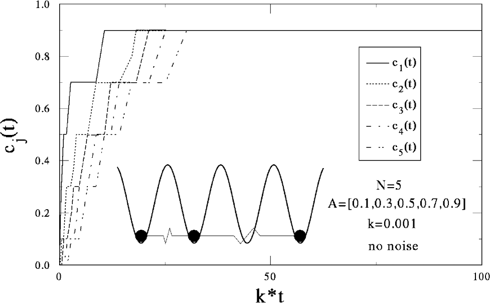
FIG. 1.: Plot of curvatures $c_{j}(t)=k(x_{j+1}(t)-2x_{j}(t)+x_{j-1}(t))$ versus scaled time variable $k*t$ for Eqs. (1) with no noise and boundary conditions $x_{0}(t)=0$, $x_{N+1}(t)=x_{N}(t)$, starting from the initial condition $x_{j}(t=0)=0$ for $j=1,\ldots,N$. System parameters are given on the plot. The horizontal regions in the graphs occur when the fractional part of one of the curvature values equals the fractional part of one of the values of $A$. Notice that while the balls spend some time on each of the memory values, all the curvature values eventually end up at the single memory value $0.9$. Inset: sketch of balls and springs in periodic potential, a physical realization of Eqs. (1).

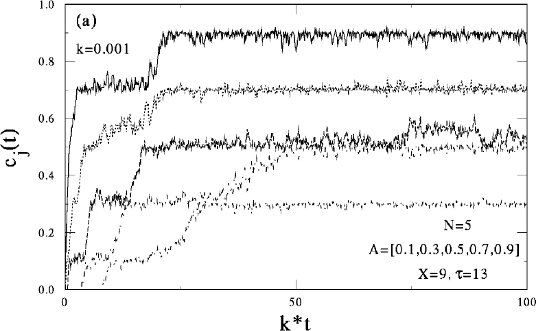
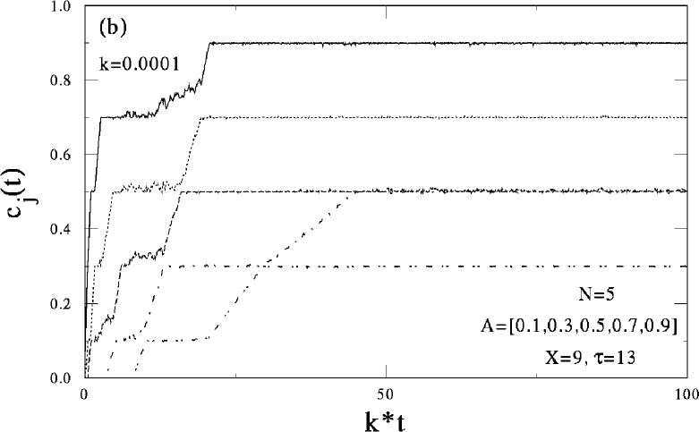
FIG. 2.: Effect of adding noise to the system of Figure 1, again starting from the initial condition $x_{j}(t=0)=0$ for $j=1,\ldots,N$. On each panel the curves from top to bottom are $c_{1}(t)$, $\ldots$, $c_{5}(t)$. Unlike the case without noise, four memory values (0.9, 0.7, 0.5, and 0.3) all appear to persist out to long times. In (a), one of the curvature variables fluctuates far from memory values, indicating that noise can destabilize as well as stabilize memories. In (b), the parameter $k$ has been reduced, with all other parameters held fixed; here, the fluctuations in the curvatures are much smaller.

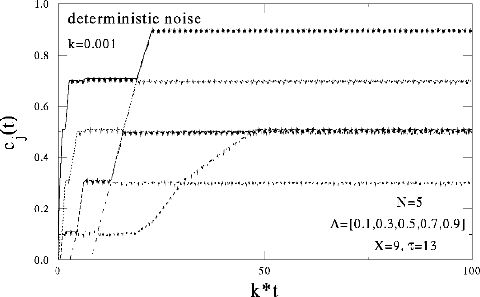
FIG. 3.: Time evolution of the curvatures in a system of five particles ($N=5$) in the presence of deterministic “noise.” Except for order of the sequence of noise kicks, the system is identical to that in Fig. 2(a). The curves from top to bottom are $c_{1}(t)$, $\ldots$, $c_{5}(t)$. Note the similarity in the large scale features of these curves, where deterministic noise has been applied, with those with random noise, shown in Fig. 2.

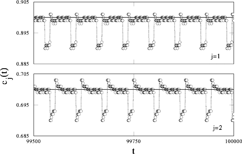
FIG. 4.: Plot of two curvatures in the system of Figure 3 versus time on an expanded scale. Parameter values are $k=0.001$, $N=5$, $A=[0.1,0.3,0.5,0.7,0.9]$, $X=9$, $\tau=13$, with deterministic noise. The plots show $c_{1}$ and $c_{2}$ versus time after the long-term behavior has been reached. The behavior is periodic; the period is $65$ time steps, the length of one noise cycle for $N=5$ and $\tau=13$.

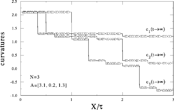
FIG. 5.: Numerical results for the curvature values observed at long times as a function of the parameter $X/\tau$ for a system with $N=3$ and deterministic noise. For these computations $k=0.0003$, but the results are insensitive to $k$ when $k$ is small. The solid lines are the analytical prediction for these curvature values using Eqs. (25) and (21). The number and value of the stable memory values for given $X/\tau$ can be read from the graph, keeping in mind that curvature values which differ by an integer are on the same memory. For example, for $X/\tau=3$, $c_{1}\approx 1.3,c_{2}\approx 0.3,$ and $c_{3}\approx-0.7$, so there is one stable memory for these parameter values. Other choices of $X/\tau$ (such as $X/\tau=1.1$) yield more stable memories.

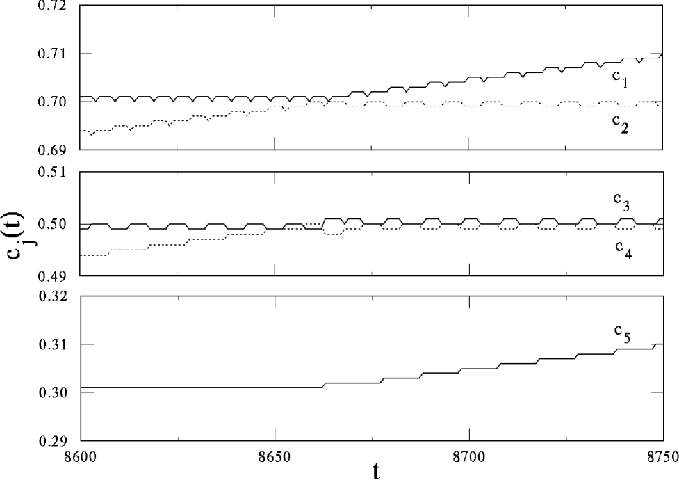
FIG. 6.: Plot of curvatures versus time on an expanded scale during the evolution of the noiseless system of Figure 1. Parameter values are $k=0.001$, $N=5$, $A=[0.1,0.3,0.5,0.7,0.9]$. The particles can be divided into two types—those whose curvatures oscillate periodically in time about memory values (for one case, $c_{5}$, the curvature on the memory is actually time-independent until $c_{4}$ hits a memory at $t\sim 8660$), and those in transit between memory values.

REFERENCES

- [1] S.N. Coppersmith et al., Phys. Rev. Lett. 78, 3983 (1997).
- [2] S.N. Coppersmith, Phys Rev. A 36, 3375 (1987).
- [3] This relationship is easiest to understand in the limit that the potential is turned off during each force pulse. During each pulse, each particle translates by an amount proportional to the total force on it (applied force plus spring force). causing each particle to fall into the nearest well bottom, at the closest integer.
- [4] A recent review of some aspects of this model is L.M. Floría and J.J. Mazo, Adv. Phys. 45, 505-598 (1996).
- [5] See, e.g., G. Grüner, Rev. Mod. Phys. 60, 1129 (1988), R.E. Thorne, Physics Today 49:5, 42 (1996), and references therein.
- [6] Experiments demonstrating single memory encoding in CDW’s are presented in R.M. Fleming and L.F. Schneemeyer, Phys. Rev. B 33, 2930 (1986), and S.E. Brown et al, Solid State Comm. 57,165 (1986).
- [7] S.N. Coppersmith and P.B. Littlewood, Phys. Rev. B 36, 311 (1987).
- [8] The signs here are chosen so that positive corresponds to the balls being moved closer to the nail (each noise event causing a reduction in strain).
- [9] P. Bak, C. Tang, and K. Wiesenfeld, Phys. Rev. Lett. 59, 381 (1987), J. Carlson and J. Langer, Phys. Rev. Lett. 62, 2632 (1989), A.V.M. Herz and J. J. Hopfield, Phys. Rev. Lett. 75, 1222 (1995).
- [10] C. Tang et al, Phys. Rev. Lett. 58, 1161 (1987).
- [11] The boundary conditions for the ’s is obtained most easily by writing . The requirement for all can be satisfied by setting for all .
-
[12]
Let
be the position of the particle and be the
unstretched length of the spring between particles and
at time , so that the spring force exerted by the
spring on particle at time is
.
(The sign follows because
the force pulses push the particles backward, so that
the ’s are negative and the curvatures
(spring forces) are positive.)
The must satisfy:
Defining , with , we find(76) (77)
If at time , the unstretched length of the spring, , is increased by , we obtain Eq. (8).(78) (79) - [13] See, e.g., S. G. Lemay, M.C. De Lind van Wijugaarden, T.L. Adelman, R.E. Thorne, Phys. Rev. B 57, 12781-91 (1988), and references therein; S. Ramakrishna, M.P. Maher, V. Ambegaokar, U. Eckern, Phys. Rev. Lett. 68, 2066-2069 (1992).
- [14] L. Pietronero and S. Strassler, Phys. Rev. B 28, 5683 (1983).
- [15] D.S. Fisher, Phys. Rev. B 31, 1396 (1985).
- [16] P.B. Littlewood, Phys. Rev. B 33, 6694 (1986).
- [17] It is straightforward to generalize the analysis presented here to include the case where an is an integer, but at the cost of a more cumbersome notation.
- [18] This restriction excludes only a set of ’s of measure zero.
- [19] To make and different at long times, one needs to apply forces at the ends whose magnitudes or durations are accelerating at different rates. Using force pulses which are inhomogeneous in space but independent of time does not lead to multiple memories, as can be seen from the results with no noise and the nailed boundary condition.
- [20] D. DiCarlo, R.E. Thorne, E. Sweetland, M. Sutton, J.D. Brock, Phys. Rev. B 50, 8288-96 (1994), and references therein.
-
[21]
One way to derive this solution is to define
.
Using Eq. (58), one finds that the obey
which has the solution(80) (81) - [22] L. P. Kadanoff and G. Baym, Quantum Statistical Mechanics: Green’s Function Methods in Equilibrium and Nonequlibrium Problems (W.A. Benjamin, New York, 1962).
- [23] S. Doniach and E.H. Sondheimer, Green’s Functions for Solid State Physicists (Benjamin/Cummings, Reading, MA, 1974).
- [24] M. Abramowitz and C.A. Stegun (Eds.), Handbook of Mathematical Functions with Formulas, Graphs, and Mathematical Tables, 9th printing (Dover, New York 1972).
- [25] S. Chandrasekhar, Rev. Mod. Phys. 15, 1 (1943).
- [26] This is clearly possible when the boundary conditions specify and . Our nailed boundary condition of one free and one fixed end is equivalent to fixing , with .