[

Magnetic skyrmion lattices in heavy fermion superconductor UPt₃

Abstract

Topological analysis of nearly SO(3)_spin symmetric Ginzburg–Landau theory, proposed for UPt₃ by Machida et al, shows that there exists a new class of solutions carrying two units of magnetic flux: the magnetic skyrmion. These solutions do not have singular core like Abrikosov vortices and at low magnetic fields they become lighter for strongly type II superconductors. Magnetic skyrmions repel each other as $1/r$ at distances much larger then the magnetic penetration depth $\lambda,$ forming a relatively robust triangular lattice. The magnetic induction near $H_{c1}$ is found to increase as $(H-H_{c1})^{2}$. This behavior agrees well with experiments.

]

Heavy fermion superconductors have surprising properties on both the microscopic and the macroscopic level. Charge carrier’s pairing mechanism is unconventional. The vortex state is also rather different from that of s-wave superconductors: there exist unusual asymmetric vortices, and phase transitions between numerous vortex lattices take place[1]. For the best studied material UPt₃ several phenomenological theories have been put forward [2, 3, 4] which utilize a multicomponent order parameter. In particular, great effort has been made to qualitatively and quantitatively map the intricate $H-T$ phase diagram. Most attention has been devoted to the region of magnetic fields near $H_{c2}$.

Magnetization curves of  UPt₃ near $H_{c1}$ are also rather unusual (see Fig.1). Theoretically, if the magnetization is due to penetration of vortices into a superconducting sample then one expects $-4\pi M$ to drop with an infinite derivative at $H_{c1}$ (dotted line). On the other hand experimentally $-4\pi M$ continues to increase smoothly (squares and triangles represent rescaled data taken from refs. [5] and [6] respectively). Such a behavior was attributed to strong flux pinning or surface effects [5]. However both experimental curves in Fig.1, as well as the other ones found in literature, are close to each other if plotted in units of $H_{c1}$. There might be a more fundamental explanation of the universal smooth magnetization curve near $H_{c1}$. If one assumes that fluxons are of unconventional type for which interaction is long range  then precisely this type of magnetization curve is obtained.

Magnetization near $H_{c1}$ due to fluxons carrying $N$ units of flux $\Phi_{0}\equiv hc/2e$, with line energy $\varepsilon$ and mutual interaction $V(r)$, is found by minimizing the Gibbs energy of a very sparse triangular lattice:

$$G(B)=\frac{B}{N\Phi_{0}}\left[\varepsilon+3V(a)\right]-\frac{BH}{4\pi},$$ (1)

where $a=(\Phi_{0}/B\sqrt{3})^{\frac{1}{2}}$ is lattice spacing. When $V(r)\sim\exp[-\lambda r],$ the magnetic induction has the conventional behavior $B\sim\left[\log\left(H-H_{c1}\right)\right]^{-2}$[7], while if it is long range, $V(r)\sim 1/r^{n},$ then one finds $B\sim\left(H-H_{c1}\right)^{n+1}$. The physical reason for this different behavior is very clear. For a short range repulsion, if one fluxon penetrated the sample, many more can penetrate almost with no additional cost of energy. This leads to the infinite derivative of magnetization. On the other hand for a long range interaction making a place for each additional fluxon becomes energy consuming. Derivative of magnetization thus becomes finite.

It is generally assumed that although vortices in UPt₃ differ from the usual Abrikosov vortices in many details [8] two important characteristics are preserved. First, their size $\lambda$ is well defined: magnetic field and interactions between vortices vanish exponentially beyond this length. Second, their energy is proportional to $\log\kappa$. However, in this note we show on the basis of topological analysis of a model by Machida et al. [9] that there exists an additional class of fluxons which we call magnetic skyrmions. They carry two units of magnetic flux $N=2$ and do not have a singular core, similar to ATC texture in superfluid ³He [10]. We show that their line energy $\varepsilon\approx 2\varepsilon_{0}$, $\varepsilon_{0}\equiv\left(\Phi_{0}/4\pi\lambda\right)^{2}$ is independent $\kappa$ and is smaller than that of Abrikosov vortices for strongly type II superconductors like UPt₃ ($\kappa\sim 50$). Magnetic skyrmion lattice becomes the ground state at low magnetic fields $(H-H_{c1})/H_{c1}\ll 1$. We further find that the repulsion of magnetic skyrmions is, in fact, long range: $V(r)\sim 1/r$. This allows us to produce a nice fit to the magnetization curve (solid line in Fig.1) which is universal (independent of $\kappa$).

The order parameter in the weak spin–orbit coupling model of UPt₃ is a three dimensional complex vector: $\psi_{i}(\vec{r})$[2]. The Ginzburg–Landau free energy reads:

$$F=F_{sym}+\Delta F,$$ (2)

$$F_{sym}=-\alpha\psi_{i}\psi_{i}^{\ast}+\frac{\beta_{1}}{2}(\psi_{i}\psi_{i}^{\ast})^{2}+\frac{\beta_{2}}{2}|\psi_{i}\psi_{i}|^{2}$$ (3)

$$+K_{1}\left(|{\cal D}_{x}\psi_{i}|^{2}+|{\cal D}_{y}\psi_{i}|^{2}\right)+K_{2}\left|{\cal D}_{z}\psi_{i}\right|^{2}+\frac{1}{8\pi}B_{j}^{2},$$ (4)

$$\Delta F=-\gamma|\psi_{x}|^{2}-\lambda|\psi_{z}|^{2}+\frac{\Delta\chi}{2}|\psi_{i}B_{i}|^{2}$$ (5)

$$+\sum_{i=x,y}\left[k_{1}^{i}\left(|{\cal D}_{x}\psi_{i}|^{2}+|{\cal D}_{y}\psi_{i}|^{2}\right)+k_{2}^{i}\left|{\cal D}_{z}\psi_{i}\right|^{2}\right],$$ (6)

where ${\cal D}_{j}\equiv\partial_{j}-i(2{e}/{\hbar c})A_{j}$ and $B_{j}=(\nabla\times\vec{A})_{j}$. We separated eq.(2) into a symmetric part $F_{sym}$ which is invariant under the spin rotation group   SO(3)_spin acting on the index $i$ of the order parameter, and into terms breaking the SO(3)_spin symmetry (anisotropy, coupling to antiferromagnetic spin fluctuations and spin-orbit coupling). Although $\Delta F$ is crucial in explaining the double superconducting phase transition in UPt₃ at zero external magnetic field and the shape of $H_{c2}(T)$ curve on the $H-T$ phase diagram, it can be considered as a small perturbation in the low temperature superconducting phase (phase B) well below its critical temperature $T\ll T_{c}^{-}\simeq.45$ K and at low magnetic fields $H\simeq H_{c1}$. Indeed, estimation of coefficients of $\Delta F$ at $T=T_{c}^{-}/2$ yields: $\gamma/\alpha\simeq.2,\lambda/\alpha\simeq.05$ and $\left(\frac{\Delta\chi}{2}H_{c1}^{2}\right)/\left(\frac{\alpha^{2}}{2\beta_{1}}\right)\simeq 10^{-6}$, and also $k\ll K$ [2]. Therefore, in a certain range of magnetic fields and temperatures there is an approximate O(3) symmetry and we first turn to minimize $F_{sym}$.

In the vacuum of phase B the order parameter is $\vec{\psi}=\psi_{0}(\vec{n}+i\vec{m})/\sqrt{2}$,$\psi_{0}^{2}\equiv\alpha/\beta_{1}$, $\;\vec{n}\perp\vec{m}$, $\vec{n}^{2}=\vec{m}^{2}=1.$ Stability requires: $\alpha>0$, $\beta_{1}>0$ and $\beta_{2}>-\beta_{1}.$ The symmetry breaking pattern of phase B is as follows. Both the spin rotations SO(3)_spin and the U(1) gauge symmetries are spontaneously broken, but a diagonal subgroup U(1) survives. The subgroup consists of combined transformations: rotations by angle $\vartheta$ around the axis $\vec{l}$ $\equiv\vec{n}\times\vec{m}$ accompanied by gauge transformations $e^{i\vartheta}$. Each vacuum state is specified by orientation of a triad of orthonormal vectors $\vec{n},$ $\vec{m},$ $\vec{l}$. The vacuum manifold is therefore isomorphic to SO(3). Topological defects might be of two kinds: regular and ”singular”. To find regular topological line defects, it is enough to consider the London approximation [10], i.e. to assume that the order parameter gradually changes in space from one vacuum to another. The triad $\vec{n},$ $\vec{m},$ $\vec{l}$ then becomes a field. The Abrikosov vortex is a singular defect: it has a core where the modulus of the order parameter vanishes and energy diverges logarithmically. Accordingly, a cutoff parameter – the correlation length – should be introduced and one obtains $\log\kappa$ dependence for the vortex line energy. This fact alone means that if there exists a regular solution it is bound to become energetically favorable for large enough $\kappa$. Below we consider a situation when the external magnetic field is oriented along $z$ axis and all configurations are translationally invariant in this direction. We use dimensionless units: $r\equiv\lambda\tilde{r}$, $A\equiv\left(\Phi_{0}/2\pi\lambda\right)\tilde{A}$, $B\equiv\left(\Phi_{0}/2\pi\lambda^{2}\right)\tilde{B}$ and $F=(\varepsilon_{0}/2\pi\lambda^{2})\tilde{F},$ where $\lambda\equiv(\Phi_{0}/2\pi)\sqrt{\beta_{1}/4\pi\alpha K_{1}}$ (the tilde will be dropped hereafter). The free energy takes form

$$F_{L}=1/2\left(\partial_{k}\vec{l}\right)^{2}+\left(\vec{n}\partial_{k}\vec{m}-A_{k}\right)^{2}+B_{k}^{2}$$ (7)

and the field equations are

$$n_{p}\vec{\nabla}m_{p}\!\!-\vec{A}=\vec{\nabla}\times\left(\vec{\nabla}\times\vec{A}\right)=\vec{j},$$ (8)

$$\Delta\vec{l}-\vec{l}(\vec{l}\cdot\Delta\vec{l})+2j_{k}(\vec{l}\times\partial_{k}\vec{l})=0.$$ (9)

Eq.(8) shows that the superconducting velocity is given by $n_{p}\vec{\nabla}m_{p}=-\vec{\nabla}\vartheta$, where the angle $\vartheta$ specifies the orientation of vector $\vec{n}$ or $\vec{m}$ in the plane perpendicular to $\vec{l}$ (see insert in Fig.2). Thus, $\vartheta$ is the superconducting phase.

Now we proceed to classify the boundary conditions. Magnetic field vanishes at infinity, while topology of the orientation of the triad $\vec{n},$ $\vec{m},$ $\vec{l}$ at different distant points is described by the first homotopy group of vacuum manifold: $\pi_{1}$(SO(3))$=$Z₂ [10]. It yields a classification of solutions into two topologically distinct classes (”odd” and ”even”). This classification is too weak, however, for our purposes because it does not guarantee nontrivial flux penetrating the plane. We will see that configurations having both ”parities” are of interest. In the presence of the magnetic flux possible configurations are further constrained by the flux quantization condition. The vacuum manifold is naturally factored into SO(3)$\rightarrow$SO(2)$\otimes$S₂ where the S₂ is set of directions of $\vec{l}$ and the SO(2) is the superconducting phase $\vartheta$. For a given number of flux quanta $N$, the phase $\vartheta$ makes $N$ windings at infinity, see Fig. 2. The first homotopy group of this part is therefore fixed: $\pi_{1}$(SO(2))$=$Z. If, in addition, $\vec{l}$ is constant, there is no way to avoid singularity in the phase $\vartheta$ where $|\vec{\psi}|=0$. However, general requirement that a solution has finite energy is much weaker. It tells us that the direction of $\vec{l}$ should be fixed only at infinity [11]. The relevant homotopy group is nontrivial: $\pi_{2}$(S₂)$=$Z. The second homotopy group appears because fixing $\vec{l}$ at infinity (say, up) effectively ”compactifies” two dimensional physical space into S${}_{2}.$ Unit vector $\vec{l}$ winds towards the center of the texture. The new topological number is $Q=(1/8\pi)\int\varepsilon_{ij}\,\vec{l}\,\left(\partial_{i}\vec{l}\times\partial_{j}\vec{l}\right)d^{2}r$.  Therefore, all configurations fall into classes characterized by the two integers $N$ and $Q$. For regular solutions, however, these two numbers are not independent. Upon integrating the supercurrent equation, eq.(8) along a remote contour and making use of the identity $\varepsilon_{pqs}l_{p}(\partial_{i}l_{q})(\partial_{j}l_{s})=(\partial_{i}n_{p})(\partial_{j}m_{p})-(\partial_{i}m_{p})(\partial_{j}n_{p}),$ we obtain: $Q=N/2.$ We call these regular solutions magnetic skyrmions.

The lowest energy solution within the London approximation corresponds to $N/2=Q=-1$ (or $N/2=Q=+1$). We analyze a cylindrically symmetric situation and choose the triad $\vec{n},$ $\vec{m},$ $\vec{l}$ in the form:

$$\vec{l} = \vec{e}_{z}\cos\Theta(\rho)+\vec{e}_{\rho}\sin\Theta(\rho),$$ (10)

$$\vec{n} = \left(\vec{e}_{z}\sin\Theta(\rho)-\vec{e}_{\rho}\cos\Theta(\rho)\right)\sin\varphi+\vec{e}_{\varphi}\cos\varphi,$$ (11)

$$\vec{m} = \left(\vec{e}_{z}\sin\Theta(\rho)-\vec{e}_{\rho}\cos\Theta(\rho)\right)\,\cos\varphi-\vec{e}_{\varphi}\sin\varphi,$$ (12)

where $\rho$ and $\varphi$ are polar coordinates and $\Theta=\widehat{\vec{e}_{z}\vec{l}}$. Boundary conditions are: $\Theta(0)=\pi$ and $\Theta(\infty)=0$. The vector potential is given by $\vec{A}=A(\rho)\vec{e}_{\varphi}$. The general form of such a configuration is shown in Fig.2. The unit vector $\vec{l}$ (solid arrows) flips its direction from up to down as it moves from infinity toward the origin. The phase $\vartheta$ (arrow inside small circles in Fig.2) winds twice while completing an ”infinitely remote” circle. If in eq. (7) only the first term were present we would deal with a standard $SO(3)$ invariant nonlinear $\sigma$-model [12]. Being scale invariant, it possesses infinitely many pure skyrmion solutions $\Theta_{s}(\rho;\delta)=2\arctan(\delta/\rho),$ which have the same energy equal to $2$ (in units of $\varepsilon_{0}$) for any size $\delta$ of a skyrmion. However, in the present case the structure of the order parameter is more complex and the above degeneracy is lifted  by the second and third terms of eq. (7).

Below we make use of the functions $\Theta_{s}(\rho;\delta)$ to explicitly construct the variational configurations. We show that as size of these configurations increases the energy is reduced to a value arbitrarily close to the absolute minimum of $\varepsilon_{ms}=2$. Substituting eq.(11) into eq.(7) and integrating over the $x-y$ plane we obtain the energy of the magnetic skyrmion in the form: $\varepsilon_{ms}=\varepsilon_{s}+\varepsilon_{cur}+\varepsilon_{mag}$, where $\varepsilon_{s}\equiv\int\rho d\rho\left(\Theta^{\prime 2}/2+\sin^{2}\Theta/2\rho^{2}\right)$, $\varepsilon_{cur}\equiv\int\rho d\rho\left[(1+\cos\Theta)/\rho+A\right]^{2}$ and $\varepsilon_{mag}\equiv\int\rho d\rho\left(A/\rho+A^{\prime}\right)^{2}$. The first term $\varepsilon_{s}$ is the same as in nonlinear $\sigma$-model without magnetic field. It is bound from below by $2$, the energy of a pure skyrmion. The second term $\varepsilon_{cur}$, the ”supercurrent” contribution, is positive definite. One still can maintain zero value of this term when the field $\Theta(\rho)$ is a pure skyrmion $\Theta_{s}(\rho;\delta)$ of certain size $\delta$. Assuming this one gets: $A(\rho)=-(1+\cos\Theta)/\rho=-2\rho/(\rho^{2}+\delta^{2})$. The third term, the magnetic field contribution (which is also positive definite), becomes $\varepsilon_{mag}=8/3\delta^{2}$. It is clear that when $\delta\rightarrow\infty$ we obtain energy arbitrarily close to the lower bound: $\varepsilon_{ms}\leq 2+8/3\delta^{2}\rightarrow 2$. Single magnetic skyrmion therefore blows up.

If many magnetic skyrmions are present, then their interactions can stabilize the system. They repel each other, as we will see shortly, and therefore form a lattice. Since they are axially symmetric, the interaction is axially symmetric and thus a triangular lattice is expected. Assume that the lattice spacing is $a$. At the boundaries of the hexagonal unit cells the angle $\Theta$ is zero, while at the centers it is $\pi$. The magnetic field $B$ is continuous on the boundaries. Therefore, to analyze a magnetic skyrmion lattice we should solve eqs.(8)–(9) on the unit cell with these boundary conditions demanding that two units of flux pass through the cell (by adjusting the value of magnetic field on the boundary). We have approximated the hexagonal unit cell by a circle of radius $R=3^{3/4}a/\sqrt{\pi}$ and the same area, and performed numerical integration of the equations

$$A^{\prime\prime}+\frac{A^{\prime}}{\rho}-\frac{A}{\rho^{2}}-A-\frac{1+\cos\Theta}{\rho} = 0,$$ (13)

$$\Theta^{\prime\prime}+\frac{\Theta^{\prime}}{\rho}+\frac{\sin\Theta}{\rho}\left(\frac{2+\cos\Theta}{\rho}+2A\right) = 0,$$ (14)

which follow from the cylindrically symmetric Ansatz of eq.(11). Calculations for $R$ from $R=5$ till $R=600$ were done by means of a finite element method. The energy per unit cell in a wide range of $R$ is satisfactory described (deviation at $R=10$ is $1\%$) by the function $\varepsilon_{cell}\simeq 2+5.62/R$. Note that in the limit $R\rightarrow\infty$ we recover our previous variational estimate: $\varepsilon_{cell}\rightarrow\varepsilon_{ms}=2.$ The dominant contribution to magnetic skyrmion energy at large $\ R$ comes from the first term $\varepsilon_{s}$, similar to the analytical variational state described above. The contribution to $\varepsilon_{cell}$ from magnetic field, $\varepsilon_{mag}$, is small for large $R$ but becomes significant in denser lattices. The most interesting feature of the solution is that the supercurrent contribution $\varepsilon_{cur}$ to the energy of magnetic skyrmion is negligibly small for all considered values of $R$. This is to be compared with the usual Abrikosov vortex where at high $\kappa$ the total energy is dominated by magnetic and supercurrent contributions which are of the same order of magnitude. Most of the flux goes through the region where the vector $\vec{l}$ is oriented upwards. In other words, the magnetic field is concentrated close to the center of a magnetic skyrmion.

Line energy of Abrikosov vortices $\varepsilon_{v}$ for the present model was calculated numerically (beyond London approximation) in [13]. For $\kappa=20$ and  $50$ we obtain $2\varepsilon_{v}/\varepsilon_{ms}\approx 3.5$ and $4.4$ respectively. Therefore we expect that the lower critical field of UPt₃ is determined by magnetic skyrmions: $h_{c1}=\varepsilon_{ms}/2N$. Returning to physical units,

$$H_{c1}=\Phi_{0}/4\pi\lambda^{2}.$$ (15)

To find magnetization, we now utilize eq.(1). Interactions among magnetic skyrmions follows easily from the energy of a unit cell of the hexagonal lattice: $V(r)=2(\varepsilon_{cell}-2)/6\simeq 1.87/r$. The resulting averaged magnetic induction, in units of $\Phi_{0}/2\pi\lambda^{2}$, reads

$$B\simeq 0.25\left(H/H_{c1}-1\right)^{2}.\;\;$$ (16)

This agrees very well with the experimental results, see Fig.1. For fields higher then several $H_{c1}$ London approximation is not valid anymore since magnetic skyrmions will start to overlap. In this case one expects that ordinary Abrikosov vortices, which carry one unit of magnetic flux, become energetically favorable. The usual vortex picture has indeed been observed at high fields by Yaron et al. [14] Curiously, our result is similar to conclusions of Burlachkov et al.[15] who investigated stripe-like (quasi one dimensional) spin textures in triplet superconductors. Having established the magnetic skyrmion solution of $F_{sym}$ we next estimated how it is influenced by various terms of $\Delta F$ eqs.(5)–(6). It was found that these perturbations do not lead to destabilization of a magnetic skyrmion.

In conclusion, we have performed a topological classification of the solutions in SO(3)_spin symmetric GL free energy. This model, with addition of very small symmetry breaking terms, describes heavy fermion superconductor UPt₃ and possibly other p-wave superconductors. A new class of topological solutions in weak magnetic field was identified. These solutions, magnetic skyrmions, do not have normal core. At small magnetic fields the magnetic skyrmions are lighter then Abrikosov vortices and therefore dominate the physics. Magnetic skyrmions repel each other as $1/r$ at distances much larger then magnetic penetration depth forming a relatively robust triangular lattice. $H_{c1}$ is reduced by a factor $\log\kappa$ as compared to that determined by usual Abrikosov vortex (see eq.(15)).

The following characteristic features, in addition to the slope of the magnetization curve, can allow experimental identification of a magnetic skyrmions lattice.

1. Unit of flux quantization is $2\Phi_{0}$.

2. Superfluid density $|\vec{\psi}|^{2}$ is almost constant throughout the mixed state. This can be tested using STM techniques.

3. Due to the fact that there is no normal core, in which usually dissipation and pinning take place, one expects that pinning effects are reduced.

It is interesting to note that our results are actually applicable to another model of UPt₃ with accidentally degenerate AE representations [16]. Although this model adopts the strong spin–orbit coupling scheme,  it has a structure closely related to $F_{sym}$ of eqs.(3)–(4) at low temperatures where both order parameters become of equal importance and can be viewed as a single three dimensional order parameter.

The authors are grateful to B. Maple for discussion of results of Ref. 5, to L. Bulaevskii, T.K. Lee and J. Sauls for discussions and to A. Balatsky for hospitality in Los Alamos. The work is supported by NSC, Republic of China, through contract #NSC86-2112-M009-034T.

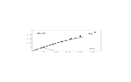
FIG. 1.: Magnetization of magnetic skyrmion lattice (solid line) and experimental data for UPt₃ from Ref.5 (squares) and Ref.6 (triangules). Magnetization of Abrikosov vortex lattice (dotted line) is given for comparison.

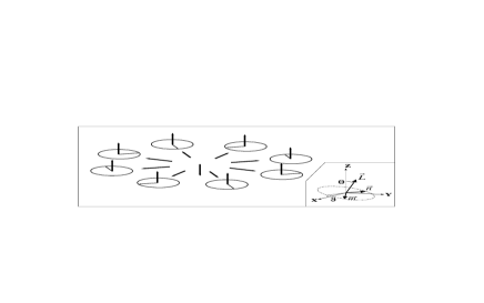
FIG. 2.: Configuration of a magnetic skyrmion. Solid arrows represent $\vec{l}$ field while the ”clocks” show that phase $\vartheta$ rotates twice as an infitely remote contour is circumvented. Insert explains defintions of $\vartheta$ and $\Theta.$

REFERENCES

- [1] J.A. Sauls, Adv. Phys., 43, 113 (1994); M. Sigrist, K. Ueda, Rev. Mod. Phys. 63, 239 (1991); I.A. Luk’yanchuk, M.E. Zhitomirsky, Supercond. Rev. 1, 207 (1995).
- [2] K.Machida, M.Ozaki, Phys. Rev. Lett. 66, 3293 (1991); K.Machida, T.Ohmi, M.Ozaki, J. Phys. Soc. Jpn. 62, 3216 (1993); T.Ohmi, K.Machida; ibid 65, 4018 (1996).
- [3] J.A.Sauls, J. Low Tem. Phys. 95, 153 (1994).
- [4] K.A.Park, R.Joynt, Phys. Rev. Lett. 74, 4734 (1995).
- [5] A.Amann, A.C.Mota, M.B.Maple, H.v.Lohneysen, Phys. Rev. B57, 3640 (1998).
- [6] Z.Zhao et al., Phys. Rev. Lett. 43, 13720 (1991).
- [7] M.Tinkham, Introduction to superconductivity (McGraw–Hill, 1996).
- [8] T.A.Tokuyasu, D.W.Hess, J.A.Sauls, Phys. Rev. B41, 8891 (1990); T.A.Tokuyasu, J.A.Sauls, Physica B 165 & 166, 347 (1990); Yu.S.Barash, A.S.Mel’nikov, Sov. Phys. JETP 73 (1), 170 (1991); K.Machida, T.Fujita, T.Ohmi, J. Phys. Soc. Jpn. 62, 680 (1993).
- [9] K.Machida, T.Ohmi, J. Phys. Soc. Jpn. 67, 1122 (1998).
- [10] M.M.Salomaa, G.E.Volovik, Rev. Mod. Phys. 59, 533 (1987).
- [11] This follows from the presence of term in of eq. (7), which cannot be ”gauged away” similar to the corresponding term for the SO(2) part.
- [12] R.Rajaraman, Solitons and instantons (North-Holland, 1982).
- [13] A.Knigavko, B.Rosenstein, Phys. Rev. B58, 9354 (1998).
- [14] U.Yaron et al., Phys. Rev. Lett. 78, 3185 (1998).
- [15] L.I.Burlachkov, N.B.Kopnin, Sov. Phys. JETP 65(3), 630 (1987).
- [16] M.E.Zhitomirsky, K.Ueda, Phys. Rev. B53, 6591 (1996).