On the ubiquity of matrix-product states in one-dimensional stochastic processes with boundary interactions
Kai Klauck, Andreas Schadschneider
Institut für Theoretische Physik, Universität zu Köln, D-50937 Köln, Germany

Abstract. Recently it has been shown that the zero-energy eigenstate – corresponding to the stationary state – of a stochastic Hamiltonian with nearest-neighbour interaction in the bulk and single-site boundary terms, can always be written in the form of a so-called matrix-product state. We generalize this result to stochastic Hamiltonians with arbitrary, but finite, interaction range. As an application two different particle-hopping models with three-site bulk interaction are studied. For these models which can be interpreted as cellular automata for traffic flow, we present exact solutions for periodic boundary conditions and some suitably chosen boundary interactions.

1 Introduction

The so-called Matrix-Product Ansatz (MPA) was developed and used for the construction of Optimum Ground States (OGS) in quantum spin chains (see e.g. [1, 2, 3] and references therein). Soon the method found its way into the field of one-dimensional stochastic processes. The most prominent example in this area is the solution of the totally asymmetric simple exclusion process (TASEP) with open boundaries by Derrida, Evans, Hakim and Pasquier (DEHP) [4] , which has reached a paradigmatic status in the field of low-dimensional nonequilibrium processes.
The general principle behind the MPA for stationary states of stochastic Hamiltonians – the so-called cancelling-mechanism – was recognized by Hinrichsen et al [6], allowing the treatment of more complex reaction-diffusion systems. The cancelling-mechanism may be considered as a generalization of the OGS-concept to stochastic systems [7].
Based on this cancelling-mechanism, Krebs and Sandow (KS) [8] could prove that for stochastic processes in one dimension with nearest-neighbour interaction in the bulk and boundary fields acting only on the first and the last site, the MPA is not an Ansatz, but merely a reformulation of the problem, i.e. the stationary state of such processes can always be written as a matrix-product state (MPS). This means that – in contrast to the situation for ground states of quantum systems – (generalized) OGS are generic for stationary states of stochastic models.

Many stochastic systems arising in the context of such fields as traffic flow, granular matter, chemical reactions and biological motion have naturally an interaction, which is not restricted to nearest neighbours. However, the only example of an application of the MPA to models with an interaction range $r\geq 2$ seems to be the work of Eßler and Rittenberg [9]. These authors introduced a three-site ($r=3$) version of the cancelling-mechanism used implicitely in [4]. Preliminary studies performed by us indicated, however, that this mechanism is not the most general one and allows only the solution of some special models. Therefore it was natural to look for a generalization of the proposition by KS in order to identify the most general mechanism for arbitrary interaction range $r\geq 2$.

Indeed we found that this generalization is possible. In this letter we want to show how the mechanism of KS has to be modified to be amenable to systems with interaction range $r\geq 2$. After clarifying the cancelling-mechanism – which is the main result of this letter – the proof of our propositions is a straightforward generalization of that of KS. We therefore omit it here and postpone the details to a later publication [10]. Moreover we want to show the usefulness of our method, by solving two different particle-hopping models with three-site interaction in the bulk for periodic boundary conditions and some suitably chosen boundary interactions. Both models are interesting on their own since they can be interpreted as cellular automata describing traffic flow on a highway.

2 The generalized Krebs-Sandow proposition

We split the original proposition of Krebs and Sandow in two independent propositions A and B. The main reason is that proposition A gives a sufficient local criterion for the existence of MPS and covers stochastic processes both with boundary interactions and periodic boundary conditions. Proposition B deals with boundary interactions only where it is possible to show explicitly that the criterion of proposition A can always be fulfilled.

Consider a stochastic process on a chain consisting of $L$ sites, where each site can be in one of $m$ states. For processes in continuous time the temporal evolution of the probability vector is governed by the master equation 

$$\partial_{t}|P_{L}(t)\rangle=-\hat{H}_{L}|P_{L}(t)\rangle.$$ (1)

The linear operator $\hat{H}_{L}$ is a stochastic Hamiltonian of the form

$$\hat{H}_{L}(r)=\hat{h}_{{\rm left}}(r)+\sum_{k=1}^{L-r+1}\hat{h}_{k,k+1,\ldots,k+r-1}+\hat{h}_{{\rm right}}(r),$$ (2)

in the case of boundary interactions.
For periodic boundary conditions (p.b.c.) it has the form

$$\hat{H}^{(p)}_{L}(r)=\sum_{k=1}^{L}\hat{h}_{k,k+1,\ldots,k+r-1}.$$ (3)

The integer $r$ denotes the range of interaction in the bulk, i.e. $\hat{h}_{k,k+1,\ldots,k+r-1}$ acts on $r$ sites beginning with site $k$; $\hat{h}_{{\rm left}}(r)$ and $\hat{h}_{{\rm right}}(r)$ are boundary interactions acting on the first, respectively last, $r-1$ sites of the chain. Note that the stochastic Hamiltonians (2) and (3) are in general non-hermitian.

From now on we will only be concerned with the steady state solution of (1), which is the eigenvector $|P_{L}\rangle_{0}$ of $\hat{H}_{L}$ with eigenvalue 0. Since $\hat{H}_{L}$ is a stochastic matrix, at least one such eigenvector exists [12]. We will refer to $|P_{L}\rangle_{0}$ as zero-energy eigenvector in the following.
Moreover we address the question whether $|P_{L}\rangle_{0}$ can be written as a matrix-product state

$$|P_{L}\rangle_{0}=\frac{1}{Z_{L}}~{}\langle W|\mathcal{D}^{\otimes L}|V\rangle,$$ (4)

in the presence of boundary interactions.
For periodic boundary conditions one has to modify the ansatz to guarantee translational invariance:

$$|P_{L}\rangle_{0}=\frac{1}{Z_{L}}~{}\operatorname{Trace}[\mathcal{D}^{\otimes L}].$$ (5)

In both cases $\mathcal{D}$ is a vector of dimension $m$ with components $D_{i}$, where the $D_{i}$ are matrices acting on some auxiliary vector space $A$. $|V\rangle\in A$ and $\langle W|\in A^{*}$ are vectors in $A$ and its dual $A^{*}$, respectively.

Proposition A gives a sufficient local criterion for the existence of a matrix-product state - the so-called cancelling-mechanism. Before we proceed we have to make the following definition:

Definition.

$\mathcal{X}(r)$ is a column-vector with $m^{r-1}$ entries $X_{i_{1},i_{2},\ldots,i_{r-1}}$, where $i_{\gamma}\in\{1,2,\ldots,m\}$. The $X_{i_{1},i_{2},\ldots,i_{r-1}}$ are matrices acting on the vector space $A$ defined above. The position of $X_{i_{1},i_{2},\ldots,i_{r-1}}$ in the vector $\mathcal{X}(r)$ is given by $1+(i_{1}-1)+m(i_{2}-1)+\ldots+m^{r-2}(i_{r-1}-1)$.

Using this definition we now can formulate the first part of the generalized KS-proposition:

Proposition (A).

(i) If one can find $m$ matrices $D_{i}$ and $m^{r-1}$ matrices $\mathcal{X}(r)$ such that they fulfil

$$\hat{h}_{k,k+1,\ldots,k+r-1}(\overbrace{\mathcal{D}\otimes\mathcal{D}\otimes\cdots\otimes\mathcal{D}}^{r\text{~{}times}})=\mathcal{X}(r)\otimes\mathcal{D}-\mathcal{D}\otimes\mathcal{X}(r)$$ (6)

then $|P_{L}\rangle_{0}=\operatorname{Trace}[\mathcal{D}^{\otimes L}]$ is an zero-energy eigenvector of $\hat{H}^{(p)}_{L}(r)$ (see (3)), i.e. a stationary state of the underlying stochastic process.
(ii) If in addition to (6) one can find vectors $|V\rangle\in A$ and $\langle W|\in A^{*}$ such that

$$\langle W|\hat{h}_{l}(r)(\overbrace{\mathcal{D}\otimes\mathcal{D}\otimes\cdots\otimes\mathcal{D}}^{r-1\text{ times}})=-\langle W|\mathcal{X}(r),$$ (7)

and

$$\hat{h}_{r}(r)(\underbrace{\mathcal{D}\otimes\mathcal{D}\otimes\cdots\otimes\mathcal{D}}_{r-1\text{ times}})|V\rangle=\mathcal{X}(r)|V\rangle,$$ (8)

then $|P_{L}\rangle_{0}=\langle W|\mathcal{D}^{\otimes L}|V\rangle$ is a zero-energy eigenvector of $\hat{H}_{L}(r)$ (see (2)) with boundary interactions $\hat{h}_{{\rm left}}(r)$ and $\hat{h}_{{\rm right}}(r)$.

Proof.

The proof is a straightforward generalization of the proof in [8]. For details see [10]. ∎

Remark.

The relations (6), (7) and (8) are the most general cancelling-mechanism for the stochastic processes considered here.

In the case of boundary interactions we are able to show more. Here the matrix-product state is not an ansatz, but merely a reformulation of the fact that the stationary state is a zero-energy eigenvector of $\hat{H}_{L}(r)$ for all system lengths.

Proposition (B).

Given a stochastic process described by a stochastic Hamiltonian of the form (2) which has a unique stationary state for any system length $L$. Then the eigenstate $|P_{L}\rangle_{0}$ with eigenvalue 0 corresponding to this stationary state can be written as a matrix-product state $\langle W|\mathcal{D}^{\otimes L}|V\rangle$ with $\mathcal{D}=(D_{1},D_{2},\ldots,D_{m})^{t}$ and vectors $\langle W|$, $|V\rangle$. Moreover one finds $m^{(r-1)}$ matrices $\mathcal{X}(r)$, such that the cancelling-mechanism (6)-(8) is fulfilled.

Proof.

See [10]. As in [8] one can give an explicit construction for the operators involved. ∎

Remark.

In the case of $m=2$ and $r=3$ it is easy to see, that the cancelling-mechanism proposed in [9] is a special case of our mechanism. Using this special mechanism a proposition similar to our proposition A could be formulated. Nevertheless our mechanism has the advantage that in case of boundary interactions it leads to an algebra which is manifestly non-trivial . This stems from the fact that in the course of the proof of proposition B we construct an explicit non-trivial representation of this algebra. A discussion of this point can be found in [10].

3 Application of the proposition

We present now applications of our cancelling-mechanism by determining the stationary states of one-dimensional two-state ($m=2$) reaction-diffusion systems with three-site interactions in the bulk. In the following we investigate two models which are generalizations of the TASEP.
In the first model (model A) particles hop exclusively in one direction, say to the right, along a one-dimensional chain of length $L$ with periodic boundary conditions. Particles hop one site to the right at rate $p_{1}$, if this site is not occupied. If a particle has two empty sites in front of it, it may also move two sites to the right with rate $p_{2}$. The stochastic Hamiltonian of model A has the form (3) with $r=3$. The local operator $\hat{h}_{k,k+1,k+2}$ acts on sites $k$, $k+1$ and $k+2$ and its explicit form is given by the dynamics of the model.

Model A is of obvious relevance for the modelling of traffic flow. It can be interpreted as a model for cars which have a maximum velocity $v_{max}=2$ moving on a single-lane highway. Up to now no exact solutions of probabilistic traffic flow models with $v_{max}>1$ are known.

For the stationary state we make an ansatz of the form (5) with $\mathcal{D}=(E,D)^{t}$ where $E,D\in\operatorname{End}(V)$ and $V$ a vector space. Note that this corresponds to a grand canonical description since (5) is a superposition of states with different particle numbers. However, in our case it is not difficult to obtain results for fixed particle densities.

Using Proposition A from above, $|P_{L}\rangle_{0}$ is a stationary state if one can find 6 operators $E$, $D$, $X_{11}$, $X_{12}$, $X_{21}$ and $X_{22}$ such that they fulfil the following relations, given by the use of our cancelling mechanism

$$\begin{aligned} 0&=X_{11}E-EX_{11},\qquad\\ p_{1}DEE&=X_{12}E-EX_{21},\qquad\\ -(p_{1}+p_{2})DEE&=X_{21}E-DX_{11},\qquad\\ 0&=X_{22}E-DX_{21},\qquad\end{aligned}\begin{aligned} p_{2}DEE&=X_{11}D-EX_{12},\\ p_{1}DED&=X_{12}D-EX_{22},\\ -p_{1}DED&=X_{21}D-DX_{12},\\ 0&=X_{22}D-DX_{22}.\end{aligned}$$ (9)

The algebra given by (9) has the following one-dimensional representation with $D,E\in\mathbb{R}$:

$$\begin{aligned} D&=1-E,\qquad\\ X_{11}&=xE/D+p_{2}E^{2},\qquad\\ X_{21}&=x-p_{1}ED,\qquad\end{aligned}\begin{aligned} \ &{\phantom{strunk}}\\ X_{12}&=x\in\mathbb{R}\qquad\text{ (free parameter)},\\ X_{22}&=xD/E-p_{1}D^{2}.\end{aligned}$$ (10)

As a consequence the stationary probability distribution is a simple product measure. The particle density $\rho$ is equal to $D$ and the flow $J$ is simply given by

$$J(\rho,p_{1},p_{2})=\rho(1-\rho)[p_{1}+2p_{2}(1-\rho)],$$ (11)

which gives us the fundamental diagram, i.e. the functional relation between flow and density, at hand (see figure 1).

Flow $J$
		Density $\rho$

Figure 1: Fundamental diagram for model A with $p_{2}=1$: The dashed line corresponds to $p_{1}=0.01$ and the solid line to $p_{1}=0.99$.

Since model A does not exhibit a particle-hole symmetry, the fundamental diagrams are not symmetric with respect to $\rho=1/2$.

We have also investigated model A with parallel dynamics, which is more appropriate for traffic models [13]. Comparing the results of a so-called car-oriented mean-field theory (COMF) [14] with Monte Carlo simulations indicates that COMF gives actually the exact fundamental diagram [10].

As a next step we examined model A with open boundaries, i.e. injection of particles at the left end of a chain of length $L$, and removal of particles at the right end. For the left end we have chosen the following input rates

(12)

The symbol $E$ denotes an empty site and $D$ an occupied one.
For the right end we have chosen the output rates

(13)

Using the cancelling mechanism one gets the following relations, which have to be fulfilled in addition to (9)

$$\begin{aligned} -(\alpha_{1}+\alpha_{2})EE&=-X_{11},\qquad\\ \alpha_{2}EE-\alpha_{3}ED&=-X_{12},\qquad\\ \alpha_{1}EE&=-X_{21},\qquad\\ \alpha_{3}ED&=-X_{22},\qquad\end{aligned}\begin{aligned} \beta_{1}ED+\beta_{3}ED&=X_{11},\\ (\beta_{2}-\beta_{1})ED&=X_{12},\\ -(\beta_{3}+\beta_{2})ED+\beta_{4}DD&=X_{21},\\ -\beta_{4}DD&=X_{22}.\end{aligned}$$ (14)

We found that the one-dimensional solution (10) serves as a solution of (14), if the boundary rates are given by

$$\begin{aligned} \alpha_{1}&=p_{1}D+p_{2}DE,\qquad\\ \alpha_{2}&=p_{2}D,\qquad\\ \alpha_{3}&=\alpha_{1},\qquad\\ \end{aligned}\begin{aligned} \beta_{1}&=-\beta_{3}+p_{1}E+p_{2}E(1+E),\\ \beta_{2}&=-\beta_{3}+p_{1}+p_{2}E,\\ \beta_{4}&=p_{1}E+p_{2}E^{2},\\ \end{aligned}$$ (15)

where $\beta_{3}\in\mathbb{R}$ is a free parameter, and

$$x=p_{1}D^{2}E-p_{2}DE^{3}.$$ (16)

A more complete investigation of the properties of this model for general values of the interaction parameters will be presented in [10].

The second model we want to present (model B) has again three-site interactions in the bulk. The same model has been studied independently in [15] where equivalent results for periodic and open systems have been found. Similar to model A particles move along a chain of length $L$ exclusively in one direction. If a particle has two empty sites in front of it, it moves one site with rate $1$; if only the next site is empty, the particle performs the same move with rate $\lambda$. For $\lambda<1$ this model may be considered as a traffic flow model with a so-called ’slow-to-start rule’ (see [16] and references therein).

The stochastic process obtained from model B after a particle-hole transformation  is also very interesting [10]. Here the hopping probability depends on the occupation number of the site directly behind the particle. If the site to the left is occupied a particle moves to the right with rate $p_{2}$, if it is empty it moves with rate $p_{1}$. For $p_{1}>p_{2}$ the particles prefer to stick together which can lead to interesting clustering properties. This model might have applications for granular matter and flocking behaviour where similar interactions have been studied (see e.g. [17]).

The matrix-product ansatz is the same as for model A and we find for the bulk-algebra:

$$\begin{aligned} X_{11}E&=EX_{11},\qquad\\ DEE&=X_{12}E-EX_{21},\qquad\\ -DEE&=X_{21}E-DX_{11},\qquad\\ X_{22}E&=DX_{21},&\qquad\end{aligned}\begin{aligned} X_{11}D&=EX_{12},\\ \lambda DED&=X_{12}D-EX_{22},\\ -\lambda DED&=X_{21}D-DX_{12},\\ X_{22}D&=DX_{22}.\end{aligned}$$ (17)

For this algebra we found a two-dimensional representation which has a structure generic for a 2-cluster approximation [13]

$$E=\begin{bmatrix}e&1\\ 0&0\end{bmatrix},\qquad D=\begin{bmatrix}d&0\\ 1&0\end{bmatrix},\qquad ed=\frac{\lambda}{1-\lambda}$$ (18)

$$\begin{aligned} X_{11}&=\frac{e}{d}(d+x)E,\qquad\\ X_{21}&=\frac{x}{d}DE,\end{aligned}\begin{aligned} X_{12}&=eD+\frac{x}{d}ED,\\ X_{22}&=xD.\end{aligned}$$ (19)

Remark.

(i) It is not hard to prove, that any two operators $E$ and $D$, which fulfil

$$\begin{split}E^{2}&=eE,\\ D^{2}&=dD,\\ {\lambda}DED&={ed}D,\end{split}$$ (20)

with $e$, $d$ being c-numbers and the $X_{ij}$ defined in terms of $E$, $D$ as in (19), yield a representation of the algebra (17).
(ii) A first consequence is that any representation of the Temperly-Lieb algebra $T_{3}(\pm\sqrt{\lambda})$ gives a representation of (17). This can be seen by defining $E=e_{1}$ and $D=pe_{2}$ where $e_{1}$ and $e_{2}$ are the generators of $T_{3}(\pm\sqrt{\lambda})$ and $p$ is a free parameter.

With the use of the two-dimensional representation (18) it is possible to calculate the expectation value of any observable in the stationary state (see e.g. [4]). The fundamental diagram is given by

$$J(\rho)=\rho\left[1-\frac{1-\sqrt{1-4(1-\lambda){\rho}(1-{\rho})}}{2(1-\lambda)(1-\rho)}\right].$$ (21)

As an example we present some fundamental diagrams in figure 2.

Flow $J$
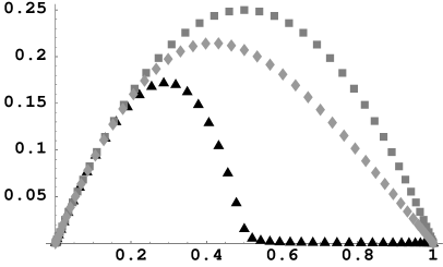
		Density $\rho$

Figure 2: Fundamental diagram of model B: squares correspond to $\lambda=0.999$, triangles to $\lambda=0.001$ and diamonds to $\lambda=0.5$ .

Again it is non-symmetric due to the lack of a particle-hole symmetry.

As for model A, we studied model B with open boundaries, having input rates

$$\lx@xy@svg{\hbox{\raise 0.0pt\hbox{\kern 17.5076pt\hbox{\ignorespaces\ignorespaces\ignorespaces\hbox{\vtop{\kern 0.0pt\offinterlineskip\halign{\entry@#!@&&\entry@@#!@\cr&&\\&&\crcr}}}\ignorespaces{\hbox{\kern-17.20828pt\raise 0.0pt\hbox{\hbox{\kern 0.0pt\raise 0.0pt\hbox{\hbox{\kern 3.0pt\raise 0.0pt\hbox{$\textstyle{|EE\cdots\ignorespaces\ignorespaces\ignorespaces\ignorespaces}$}}}}}}}\ignorespaces\ignorespaces\ignorespaces\ignorespaces{}{\hbox{\lx@xy@droprule}}\ignorespaces\ignorespaces\ignorespaces{\hbox{\kern 38.4183pt\raise 5.15138pt\hbox{{}\hbox{\kern 0.0pt\raise 0.0pt\hbox{\hbox{\kern 3.0pt\hbox{\hbox{\kern 0.0pt\raise-0.8625pt\hbox{$\scriptstyle{\alpha_{1}}$}}}\kern 3.0pt}}}}}}\ignorespaces{\hbox{\kern 71.80692pt\raise 0.0pt\hbox{\hbox{\kern 0.0pt\raise 0.0pt\hbox{\lx@xy@tip{1}\lx@xy@tip{-1}}}}}}{\hbox{\lx@xy@droprule}}{\hbox{\lx@xy@droprule}}{\hbox{\kern 41.5076pt\raise 0.0pt\hbox{\hbox{\kern 0.0pt\raise 0.0pt\hbox{\hbox{\kern 3.0pt\raise 0.0pt\hbox{$\textstyle{}$}}}}}}}{\hbox{\kern 71.80692pt\raise 0.0pt\hbox{\hbox{\kern 0.0pt\raise 0.0pt\hbox{\hbox{\kern 3.0pt\raise 0.0pt\hbox{$\textstyle{|DE\cdots}$}}}}}}}{\hbox{\kern-17.5076pt\raise-40.0pt\hbox{\hbox{\kern 0.0pt\raise 0.0pt\hbox{\hbox{\kern 3.0pt\raise 0.0pt\hbox{$\textstyle{|ED\cdots\ignorespaces\ignorespaces\ignorespaces\ignorespaces}$}}}}}}}\ignorespaces\ignorespaces\ignorespaces\ignorespaces{}{\hbox{\lx@xy@droprule}}\ignorespaces\ignorespaces\ignorespaces{\hbox{\kern 38.4183pt\raise-34.84862pt\hbox{{}\hbox{\kern 0.0pt\raise 0.0pt\hbox{\hbox{\kern 3.0pt\hbox{\hbox{\kern 0.0pt\raise-0.8625pt\hbox{$\scriptstyle{\alpha_{2}}$}}}\kern 3.0pt}}}}}}\ignorespaces{\hbox{\kern 71.5076pt\raise-40.0pt\hbox{\hbox{\kern 0.0pt\raise 0.0pt\hbox{\lx@xy@tip{1}\lx@xy@tip{-1}}}}}}{\hbox{\lx@xy@droprule}}{\hbox{\lx@xy@droprule}}{\hbox{\kern 41.5076pt\raise-40.0pt\hbox{\hbox{\kern 0.0pt\raise 0.0pt\hbox{\hbox{\kern 3.0pt\raise 0.0pt\hbox{$\textstyle{}$}}}}}}}{\hbox{\kern 71.5076pt\raise-40.0pt\hbox{\hbox{\kern 0.0pt\raise 0.0pt\hbox{\hbox{\kern 3.0pt\raise 0.0pt\hbox{$\textstyle{|DD\cdots}$}}}}}}}\ignorespaces}}}}\ignorespaces, \textstyle{|EE\cdots\ignorespaces\ignorespaces\ignorespaces\ignorespaces} \scriptstyle{\alpha_{1}} \textstyle{|DE\cdots} \textstyle{|ED\cdots\ignorespaces\ignorespaces\ignorespaces\ignorespaces} \scriptstyle{\alpha_{2}} \textstyle{|DD\cdots} \textstyle{|EE\cdots\ignorespaces\ignorespaces\ignorespaces\ignorespaces} \scriptstyle{\alpha_{1}} \textstyle{|DE\cdots} \textstyle{|ED\cdots\ignorespaces\ignorespaces\ignorespaces\ignorespaces} \scriptstyle{\alpha_{2}} \textstyle{|DD\cdots}$$ (22)

and output rates

$$\lx@xy@svg{\hbox{\raise 0.0pt\hbox{\kern 17.80692pt\hbox{\ignorespaces\ignorespaces\ignorespaces\hbox{\vtop{\kern 0.0pt\offinterlineskip\halign{\entry@#!@&&\entry@@#!@\cr&&\\&&\\&&\crcr}}}\ignorespaces{\hbox{\kern-17.5076pt\raise 0.0pt\hbox{\hbox{\kern 0.0pt\raise 0.0pt\hbox{\hbox{\kern 3.0pt\raise 0.0pt\hbox{$\textstyle{\cdots DE|\ignorespaces\ignorespaces\ignorespaces\ignorespaces}$}}}}}}}\ignorespaces\ignorespaces\ignorespaces\ignorespaces{}{\hbox{\lx@xy@droprule}}\ignorespaces\ignorespaces\ignorespaces{\hbox{\kern 38.67757pt\raise 6.1111pt\hbox{{}\hbox{\kern 0.0pt\raise 0.0pt\hbox{\hbox{\kern 3.0pt\hbox{\hbox{\kern 0.0pt\raise-1.75pt\hbox{$\scriptstyle{\beta_{1}}$}}}\kern 3.0pt}}}}}}\ignorespaces{\hbox{\kern 71.80692pt\raise 0.0pt\hbox{\hbox{\kern 0.0pt\raise 0.0pt\hbox{\lx@xy@tip{1}\lx@xy@tip{-1}}}}}}{\hbox{\lx@xy@droprule}}{\hbox{\lx@xy@droprule}}{\hbox{\kern 41.80692pt\raise 0.0pt\hbox{\hbox{\kern 0.0pt\raise 0.0pt\hbox{\hbox{\kern 3.0pt\raise 0.0pt\hbox{$\textstyle{}$}}}}}}}{\hbox{\kern 71.80692pt\raise 0.0pt\hbox{\hbox{\kern 0.0pt\raise 0.0pt\hbox{\hbox{\kern 3.0pt\raise 0.0pt\hbox{$\textstyle{\cdots ED|}$}}}}}}}{\hbox{\kern-17.5076pt\raise-40.0pt\hbox{\hbox{\kern 0.0pt\raise 0.0pt\hbox{\hbox{\kern 3.0pt\raise 0.0pt\hbox{$\textstyle{\cdots ED|\ignorespaces\ignorespaces\ignorespaces\ignorespaces}$}}}}}}}\ignorespaces\ignorespaces\ignorespaces\ignorespaces{}{\hbox{\lx@xy@droprule}}\ignorespaces\ignorespaces\ignorespaces{\hbox{\kern 38.67757pt\raise-33.8889pt\hbox{{}\hbox{\kern 0.0pt\raise 0.0pt\hbox{\hbox{\kern 3.0pt\hbox{\hbox{\kern 0.0pt\raise-1.75pt\hbox{$\scriptstyle{\beta_{2}}$}}}\kern 3.0pt}}}}}}\ignorespaces{\hbox{\kern 72.10623pt\raise-40.0pt\hbox{\hbox{\kern 0.0pt\raise 0.0pt\hbox{\lx@xy@tip{1}\lx@xy@tip{-1}}}}}}{\hbox{\lx@xy@droprule}}{\hbox{\lx@xy@droprule}}{\hbox{\kern 41.80692pt\raise-40.0pt\hbox{\hbox{\kern 0.0pt\raise 0.0pt\hbox{\hbox{\kern 3.0pt\raise 0.0pt\hbox{$\textstyle{}$}}}}}}}{\hbox{\kern 72.10623pt\raise-40.0pt\hbox{\hbox{\kern 0.0pt\raise 0.0pt\hbox{\hbox{\kern 3.0pt\raise 0.0pt\hbox{$\textstyle{\cdots EE|}$}}}}}}}{\hbox{\kern-17.80692pt\raise-80.0pt\hbox{\hbox{\kern 0.0pt\raise 0.0pt\hbox{\hbox{\kern 3.0pt\raise 0.0pt\hbox{$\textstyle{\cdots DD|\ignorespaces\ignorespaces\ignorespaces\ignorespaces}$}}}}}}}\ignorespaces\ignorespaces\ignorespaces\ignorespaces{}{\hbox{\lx@xy@droprule}}\ignorespaces\ignorespaces\ignorespaces{\hbox{\kern 38.67757pt\raise-73.8889pt\hbox{{}\hbox{\kern 0.0pt\raise 0.0pt\hbox{\hbox{\kern 3.0pt\hbox{\hbox{\kern 0.0pt\raise-1.75pt\hbox{$\scriptstyle{\beta_{3}}$}}}\kern 3.0pt}}}}}}\ignorespaces{\hbox{\kern 71.80692pt\raise-80.0pt\hbox{\hbox{\kern 0.0pt\raise 0.0pt\hbox{\lx@xy@tip{1}\lx@xy@tip{-1}}}}}}{\hbox{\lx@xy@droprule}}{\hbox{\lx@xy@droprule}}{\hbox{\kern 41.80692pt\raise-80.0pt\hbox{\hbox{\kern 0.0pt\raise 0.0pt\hbox{\hbox{\kern 3.0pt\raise 0.0pt\hbox{$\textstyle{}$}}}}}}}{\hbox{\kern 71.80692pt\raise-80.0pt\hbox{\hbox{\kern 0.0pt\raise 0.0pt\hbox{\hbox{\kern 3.0pt\raise 0.0pt\hbox{$\textstyle{\cdots DE|}$}}}}}}}\ignorespaces}}}}\ignorespaces. \textstyle{\cdots DE|\ignorespaces\ignorespaces\ignorespaces\ignorespaces} \scriptstyle{\beta_{1}} \textstyle{\cdots ED|} \textstyle{\cdots ED|\ignorespaces\ignorespaces\ignorespaces\ignorespaces} \scriptstyle{\beta_{2}} \textstyle{\cdots EE|} \textstyle{\cdots DD|\ignorespaces\ignorespaces\ignorespaces\ignorespaces} \scriptstyle{\beta_{3}} \textstyle{\cdots DE|} \textstyle{\cdots DE|\ignorespaces\ignorespaces\ignorespaces\ignorespaces} \scriptstyle{\beta_{1}} \textstyle{\cdots ED|} \textstyle{\cdots ED|\ignorespaces\ignorespaces\ignorespaces\ignorespaces} \scriptstyle{\beta_{2}} \textstyle{\cdots EE|} \textstyle{\cdots DD|\ignorespaces\ignorespaces\ignorespaces\ignorespaces} \scriptstyle{\beta_{3}} \textstyle{\cdots DE|}$$ (23)

According to our cancelling-mechanism this gives the following relations, which supplement the algebra (17):

$$\langle W|\begin{pmatrix}-\alpha_{1}EE\\ -\alpha_{2}ED\\ \alpha_{1}EE\\ \alpha_{2}ED\end{pmatrix}=-\langle W|\begin{pmatrix}X_{11}\\ X_{12}\\ X_{21}\\ X_{22}\end{pmatrix}$$ (24)

$$\begin{pmatrix}\beta_{2}ED\\ \beta_{1}DE-\beta_{2}ED\\ \beta_{3}DD-\beta_{1}DE\\ -\beta_{3}DD\end{pmatrix}|V\rangle=\begin{pmatrix}X_{11}\\ X_{12}\\ X_{21}\\ X_{22}\end{pmatrix}|V\rangle.$$ (25)

Again we found that the two-dimensional representation (18), (19) is also a representation for (24), (25) if $x$ is given by

$$x_{\pm}=\frac{\lambda}{1-\lambda}\left[e+d\pm\sqrt{(e-d)^{2}+\frac{4}{\lambda}ed}\right],$$ (26)

where $x_{+}$ and $x_{-}$ correspond to $\lambda>1$ and $\lambda<1$, respectively, and the boundary rates satisfy

$$\begin{aligned} \alpha_{1}&=1+\frac{x}{d},\qquad\\ \beta_{2}&=\beta_{3}=-\frac{x}{d},\qquad\\ \langle W|&=\left(-\frac{ed}{x},1\right),\qquad\end{aligned}\begin{aligned} \alpha_{2}&=\lambda\alpha_{1},\\ \beta_{1}&=\frac{-xe}{d(e+x)},\\ |V\rangle&=\left(1,-\frac{de}{x}-d-e\right)^{t}.\end{aligned}$$ (27)

That means that we found a line in the parameter space along which the stationary state can be written as a matrix-product state with 2-dimensional matrices. The density profiles calculated along this line are flat.

4 Conclusion

The generalization of the proposition of KS to stochastic processes with interaction range $r\geq 2$ leads to the most general cancelling-mechanism for such systems. The identification of this mechanism is one of the main results of this letter. Using this mechanism the existence of MPS for the stationary state of systems with boundary interaction is shown. As an application we were able to solve two models with three-site interactions.

These models are interesting by themselves since they might be of relevance for the description of traffic flow or granular matter. We were able to find the stationary state of the periodic system which in both cases is given by a finite-dimensional representation of the algebra obtained from the MPA.

For the open system with boundary interactions we could extend the solutions of the periodic systems for special values of the input and output rates. For general values of the boundary rates one probably needs infinite-dimensional representations.

Both models have a fundamental diagram with only one maximum. Using the argumentation of [18] one can expect that the phase diagrams of model A and B with boundary interactions essentially look like the well known phase diagram of the TASEP [4, 5].

A generalization of the KS-proposition to other update schemes [7] has been presented in [19]. A similar generalization is also possible in our case and will be presented elsewhere [10].

Acknowledgements
This work was performed within the research program of the Sonderforschungsbereich 341, Köln-Aachen-Jülich. We would like to thank K. Krebs, H. Niggemann, N. Rajewsky, V. Rittenberg, L. Santen and G. M. Schütz for useful talks and discussions.

References

• [1] Klümper A, Schadschneider A and Zittartz J 1991 J. Phys. A: Math. Gen. 24, L955; Z. Phys. B87, 281 (1992); Europhys. Lett. 24, 293 (1993)
• [2] Niggemann H and Zittartz J 1998 J. Phys. A: Math. Gen. 31, 9819
• [3] Mikeska H-J and Kolezhuk A K 1998 Int. J. Mod. Phys. 12, 2325
• [4] Derrida B, Evans M R, Hakim V and Pasquier V 1993 J. Phys. A: Math. Gen. 26, 1493
• [5] Schütz G M and Domany E 1993 J. Stat. Phys. 72, 277
• [6] Hinrichsen H, Sandow S and Peschel 1996 J. Phys. A: Math. Gen. 29, 2643
• [7] Rajewsky N, Santen L, Schadschneider A and Schreckenberg M 1998 J. Stat. Phys. 92, 151
• [8] Krebs K and Sandow S 1997 J. Phys. A: Math. Gen. 30, 3165
• [9] Essler F H L and Rittenberg V 1996 J. Phys. A: Math. Gen. 29, 3375
• [10] Klauck K and Schadschneider A, to be published
• [11] Alcaraz F C, Droz M, Henkel M and Rittenberg V 1994 Ann. Phys. 230, 250
• [12] van Kampen N G 1992 Stochastic processes in physics and chemistry, Elsevier (Amsterdam)
Oppenheim I, Shuler K E and Weiss G H 1977 Stochastic processes in chemical physics: The master equation, MIT Press (Cambridge)
• [13] Schreckenberg M, Schadschneider A, Nagel K and Ito N 1995 Phys. Rev. E51, 2939
• [14] Schadschneider A and Schreckenberg M 1997 J. Phys. A: Math. Gen. 30, L69
• [15] Antal T and Schütz G M 1998, preprint
• [16] Barlovic R, Santen L, Schadschneider A and Schreckenberg M 1998 Eur. Phys. J. 5, 793
• [17] Hayakawa H and Nakanishi K, cond-mat/9802131
• [18] Kolomeisky A B, Schütz G M, Kolomeisky E B and Straley J P 1998 J. Phys. A: Math. Gen. 31, 6911
• [19] Rajewsky N and Schreckenberg M 1997 Physica A245, 139