Recent results on Multiplicative Noise

Abstract

Recent developments in the analysis of Langevin equations with multiplicative noise (MN) are reported. In particular, we: (i) present numerical simulations in three dimensions showing that the MN equation exhibits, like the Kardar-Parisi-Zhang (KPZ) equation both a weak coupling fixed point and a strong coupling phase, supporting the proposed relation between MN and KPZ; (ii) present dimensional, and mean field analysis of the MN equation to compute critical exponents; (iii) show that the phenomenon of the noise induced ordering transition associated with the MN equation appears only in the Stratonovich representation and not in the Ito one, and (iv) report the presence of a new first-order like phase transition at zero spatial coupling, supporting the fact that this is the minimum model for noise induced ordering transitions. PACS: 05.40.+j

I Introduction

The idea that noise can induce rather non-trivial effects when added to deterministic equations it is not considered any more a shocking one. Some recently undercovered phenomena have familiarized us with the idea that strange physical mechanisms induced by noise are not as infrequent previously thought. Stochastic resonance [1], resonant activation [2], noise-induced spatial patterns [3], noise-enhanced multistability in coupled oscillators [4], and noise-induced phase transitions [5, 6, 7, 8] are just a few examples. In particular, a lot of attention has been devoted in recent years to the study of phase transitions appearing in systems the associated deterministic part of which does not exhibit any symmetry breaking. These studies were mostly limited to one-variable systems [9] until an interesting paper by Van den Broeck, Parrondo and Toral ) [5, 10] (see also [6]). These authors showed the possibility of having noise-induced transitions in spatially extended systems, and illustrated the physical mechanism originating this phenomenon: A short time instability is generated owing to the noise, and the generated non-trivial state is afterwards rendered stable by the spatial coupling [10]. In this way, by increasing the noise amplitude the instability in enhanced, and the system becomes more and more ordered: A noise-induced ordering phase transition (NIOT) is generated. In the model presented in [5] the NIOT was followed on further increasing of the noise amplitude by a second phase transition. At larger noise amplitudes, the usual role of the noise as a disorganizing source takes over and the system becomes again disordered. This is what we call a noise-induced disordering transition (NIDT). The same type of behavior has been found in other models [11, 12, 13].

In a recent paper [14] (see also [15]) we put forward that the NIOT and the NIDT have different origin. The NIOT is induced by multiplicative noise, while the NIDT is due to the presence of additive noise (even though it can also be generated in a somehow artificial way by multiplicative noise [14]). In this way we proposed the Langevin equation with multiplicative noise [16, 17], interpreted in the Stratonovich sense, as a new minimal model for NIOT. As a consequence of the previous observation we predicted and afterward confirmed the existence NIOTs in one-dimensional systems.

On the other hand, the MN Langevin equation has been proved to be related to the Kardar-Parisi-Zhang (KPZ) equation describing non-equilibrium surface growth [18]. In fact, by performing a, so called, Cole-Hopf transformation the MN Langevin equation becomes the KPZ equation with an extra wall that limits the maximum value of the height [16, 17, 19]. In this way, the critical point of the MN equation is related to a wetting transition. In fact, for large values of the control parameter, the surface escapes from the limiting wall and behaves as a KPZ surface, while for smaller values of the control parameter there is a phase in which the surface wets the wall and remains bound to it. Separating both phases there is a critical point at which the surface gets depinned or unbound [17, 20]. This critical point may either be a weak or a strong coupling fixed point depending on the noise intensity and on the system dimensionality.

In this paper we continue to explore the Langevin equation with multiplicative noise from different perspectives. The paper is structured as follows.

In section II we present the MN Langevin equation, discuss its connection with KPZ, and define the critical exponents.

In section III, we present dimensional analysis and predictions for the mean field exponents.

In section IV, by exploiting the connection with KPZ we try to observe numerically whether the MN equation does exhibit strong noise and weak noise fixed points [18, 21, 22, 23] in dimensions larger than two.

In section V we analyze the MN equation from the Ito-Stratonovich dilemma point of view and find out that the NIOT is specific of the Stratonovich representation and can not be obtained when the basic Langevin equation is intended in the Ito sense.

In section VI we show evidence of a first order phase transition at zero value of the spatial coupling. This is, the system, that in absence of spatial coupling is disordered, develops a finite value of the order parameter even for infinitesimal values of the spatial coupling constant. For all the previously studied models the spatial coupling has to be above a certain, non-zero, value to observe ordering. This supports the MN as the minimal model exhibiting a NIOT.

Finally some conclusions are presented.

II Model definition and Connection with KPZ

In this section we define the multiplicative noise Langevin equation, and review some of its properties and connections with KPZ. The MN equation is

$${\partial}_{t}\psi=-a\psi-p{\psi}^{p+1}+D{\nabla}^{2}\psi+\sigma\psi\eta$$ (1)

intended in the Stratonovich sense, where $\psi(x,t)$ is a field, and $a$, $p$, $D$ and $\sigma$ are parameters, and $\eta$ a Gaussian white noise with

$$\left<\eta(x,t)\right> = 0$$ (2)

$$\left<\eta(x,t)\eta(x^{\prime},t^{\prime})\right> = (1-\alpha\psi^{2})\delta(x-x^{\prime})\delta(t-t^{\prime}).$$ (3)

The Fokker-Planck equation associated with this reads

$${dP(\psi(x),t)\over dt}=-\int dx{\delta\over\delta\psi(x)}[-a\psi-p{\psi}^{p+1}+D{\nabla}^{2}\psi]$$ (4)

$$+ {\sigma^{2}\over 2}\int dx{\delta\over\delta\psi(x)}\sqrt{\psi}(1-\alpha\psi^{2}){\delta\over\delta\psi(x)}\sqrt{\psi}(1-\alpha\psi^{2})$$ (5)

To simplify things, we could just consider the $\alpha=0$ case for which we recover the pure multiplicative noise equation analyzed in [16, 17]. The equation with $\alpha>0$ was introduced in [14] as a prototype model exhibiting not only a NIOT but also a NIDT. This is, the order parameter does not keep on growing as noise amplitude is increased (as happens in the case $\alpha=0$). Instead, it reaches a maximum value after the NIOT, and decreases upon further increasing of noise amplitude, until a NIDT transition appears and the systems comes back to a disordered state. Phenomena of this type are often called ’reentrant transitions’.

Although, in principle, we could work in the simplest case $\alpha=0$, for technical reasons most of the numerical results present in what follows are obtained for $\alpha=1$, but it is worth stressing that, apart from the presence of the NIDT, non of the (universal) results depend on $\alpha$.

By performing a Cole-Hopf transformation ($n=\exp h$) this equation (with $\alpha=0$) reduces to:

$${\partial}_{t}h(x,t)=-a-p\exp(ph)+D{\nabla}^{2}h+D({\nabla}h)^{2}+\eta.$$ (7)

This is just a KPZ equation for a surface, defined by the height variable $h(x,t)$, except for the exponential term. This acts as a wall repelling $h$ from positive to negative values [24]. For large values of $a$ the surface escapes linearly in time from the wall and therefore, asymptotically, any effect of it is lost and the equation reduces to KPZ. In terms of $\psi$ the unbounded phase corresponds to the absorbing phase characterized by a vanishing value of its stationary order parameter value. On the other hand, for small enough values of $a$ the surface remains bound to the wall (or wetting the wall). In this the stationary value of $\psi$ takes a non-vanishing value. Separating both regimes there is a critical point which nature has been analyzed in [16, 17]. Some exponents, unexisting for KPZ, can be defined for MN. For example, if $m$ is the averaged order parameter, $\xi$ the correlation length, and $\tau$ the correlation time we have:

$$\xi \sim |a-a_{c}(\sigma)|^{\nu_{x}}$$ (8)

$$\tau \sim |a-a_{c}(\sigma)|^{\nu_{t}}$$ (9)

$$m(a) \sim |a-a_{c}(\sigma)|^{\beta_{a}}$$ (10)

$$m(\sigma) \sim |\sigma-\sigma_{c}(a)|^{\beta_{\sigma}}$$ (11)

$$m(t,a=a_{c},\sigma=\sigma_{c}) \sim t^{-\theta}.$$ (12)

Some of these exponents can be related to KPZ exponents using scaling arguments [16, 17]. For example, if $z$ is the dynamic exponent in KPZ, it was proved in [17] that $\nu_{x}=1/(2z-2)$ and $\beta_{a}>1$. On the other hand, using straightforward scaling relations we have $\theta=\beta_{a}/\nu_{t}$ and $\nu_{t}=z\nu_{x}$.

Some other exponents can be defined in analogy with what is customary in the study of systems with absorbing states [26]. These are the so called spreading or epidemic exponents. To measure them one places an initial seed in an otherwise absorbing configuration and study the evolution of the space integral of $\psi$, $N(t)$, the surviving probability $P(t)$, and the mean square deviation from the origin $R^{2}(t)$. At the critical point these scale as

$$N(t) \sim t^{\eta}$$ (13)

$$P(t) \sim t^{-\delta}$$ (14)

$$R^{2}(t) \sim t^{z^{\prime}}$$ (15)

where $\eta$, $\delta$ and $z^{\prime}=2/z$ are the spreading exponents. The following scaling law is expected to hold [27, 28]:

$$\eta+\delta+\theta=dz^{\prime}/2.$$ (16)

Searching for power law behaviors of the spreading magnitudes is a very precise way to determine the critical point.

Given the aforementioned connections between MN and KPZ, it is not surprising that their respective renormalization group (RG) flow diagrams [16] resemble very much to each other. In particular, for both of them [21, 16]: At any dimension larger than $d=2$ there are two different attractive fixed points: (i) a mean field or weak coupling (weak noise in the MN language) fixed point at which the non-linear parameter vanishes, and (ii) a strong coupling (strong noise in the MN language), non-trivial fixed point, not accessible to standard perturbative techniques [21, 29]. This means, that in particular, in $d=3$ there are two different phases depending on the noise intensity: For small intensities the system is in a weak coupling phase characterized by mean field like exponents. For noise intensities above a certain critical threshold the system is in a (rough) strong coupling phase.

The multiplicative noise equation has been studied numerically in $d=1$, and it was found that in fact the predicted relations with KPZ hold. The best values for the different critical exponents are reported in table I. However, as said before there is no roughening transition in $d=1$, and consequently it has not been observed so far in systems with MN. On what follows we present the results of extensive numerical simulations performed in three dimensional systems. By changing the noise amplitude we intend to observe the two different phases: one with exponents related to the strong coupling $3d$ KPZ exponents, and the other related to mean field (i.e. Edward Wilkinson [22, 23]) exponents.

III Scaling analysis and mean field results

Let us start discussing in this section the mean field predictions for the previously defined exponents, which already present some interesting features, and in the next section we will present numerical simulations of the three-dimensional model.

Let us fist present some naive scaling arguments. For that we define the generating functional associated to Eq. (3) [30, 31]

$$Z=\int D\psi\ D\phi\exp{(-\int{d}^{d}{\bf x}\ dt\cal L)}$$ (17)

with $\cal L$ given by

$${\cal L}={\sigma^{2}\over 2}{\phi}^{2}{\psi}^{2}+\phi\left[{\partial}_{t}\psi+(a-{\sigma^{2}\over 2})\psi+p{\psi}^{p+1}-{\nabla}^{2}\psi\right].$$ (18)

Using naive dimensional arguments, the dimensions of the time $t$, $d_{t}$, the field $\psi$, $d_{\psi}$, the response field $\phi$, $d_{\phi}$ and $\sigma^{2}$, $d_{\sigma^{2}}$ expressed in function of momenta (inverse of length) are

$${d}_{t} = -2$$ (19)

$${d}_{\psi}+{d}_{\phi} = d$$ (20)

$${d}_{\sigma^{2}}+2d-d-2 = 0\rightarrow{d}_{\sigma^{2}}=2-d.$$ (21)

From this, we conclude that the noise amplitude is marginal at the critical dimension $d_{c}=2$, irrelevant above it and relevant below $d=2$, and this result does not depend on the degree of the other nonlinearity, i.e. on $p$.

As it was shown in [27] the surviving probability in general systems with absorbing states scales as the response field. In the case of multiplicative noise the particle density in the absorbing state (i.e. in the unbound phase) decay continuously to zero, but does never reach that value (in fact $h$ goes continuously to minus infinity, and for any finite though large value of $h$, $n$ takes a non zero value). Therefore the surviving probability is equal to unity and the dimension of the response field is zero, $d_{\phi}=0$, (i.e. it scales as a constant) [27, 17]; this implies that $\delta=0$. Consequently $d_{\psi}=d$, which at the critical dimension is $d_{\psi}=2$; and therefore (using that the dimension of $a$ is $2$)

$$m\sim{[a]}^{{\beta}_{a}}\rightarrow 2=2{\beta}_{a}\rightarrow{\beta}_{a}=1.$$ (22)

Analogously $\beta_{\sigma}=1$. Observe that these results depend on the nature of the noise, and are independent on the degree of the nonlinearity in Eq. (3), i.e. on $p$. This gives us a justification, of the fact, observed numerically [17] that Eq. (3) gives the same exponents for different values of the nonlinearity $p$ (this same property is also shared by the exactly solvable zero dimensional case [32]).

On the other hand, it is interesting to observe that naive mean field approximations, not coming from power counting of the generating functional give the wrong result $\beta_{a}=\beta_{\sigma}=1/p$. In particular, in appendix A, we present different types of mean field approaches all of them leading to the same (wrong) prediction for the critical exponent $\beta$. The origin for the failure of standard mean field approaches is a rather delicate issue. We believe this is based on the fact, that even in the weak noise regime the stationary probability distribution is non-trivial; in particular it is non-symmetric and its mean value is typically far away from the most probable one. A detailed analysis of this and related issues will be discussed elsewhere.

Regarding the rest of critical indices, the mean field predictions are as follows. $\eta$ is the anomalous dimension of the field, and therefore it vanishes in mean field approximation where no diagrammatic corrections are taken into account. For the same reason, just considering naive power counting arguments: $z^{\prime}=1$, $z=2$, $\nu_{x}=1/2$, and $\theta=1$.

IV Numerical Results: the roughening transition

In this section we describe the results of extensive numerical simulations of Eq. (3) performed using the Heun method (see [33] and references therein). For that purpose space and time have been discretized using meshes of ${a}_{r}=1$ (space) and $\epsilon=0.001$ (time) respectively, and have fixed $p=2$. In $d=1$ we have chosen $D=0.2$, and $a=1$ while in $d=2$ and $d=3$ we take $D=1$, and $a=1$ (weak noise regime) or $a=18$ (strong noise regime). In all dimensions we verify that the system exhibits a NIOT as well as a NIDT for $\alpha>0$.

A $d=1$

We consider a system size $L=1000$, $D=0.2$, $a=1$, the space and time meshes are as said previously $1$ and $0.001$ respectively.

We determine some exponents, the values of which have not been previously reported in the literature, in particular $\beta_{\sigma}$, and some other with improved precision, and illustrate the methods employed to compute them.

In order to determine accurately the location of the critical point ${\sigma}_{c}$ (keeping $a$ fixed and varying $\sigma$) and the critical exponent $\beta_{\sigma}$, we determine numerically the order parameter as a function of $\sigma$ (see Fig. 1). In order to measure the order parameter we let the system evolve long enough so the stationary state is reached. Then we write $m={(\sigma-{\sigma}_{c})}^{{\beta}_{\sigma}}$, and take as critical point the value of ${\sigma}$ that maximizes the linear correlation coefficient when representing $\log(m)$ as a function of $\log(\sigma-{\sigma}_{c})$ (see Fig. 2 and 3). From the corresponding slope we determine ${\beta}_{\sigma}$ (Fig. 3). In particular we obtain ${\sigma}_{c}=1.81\pm 0.07$ and ${\beta}_{\sigma}=0.9\pm 0.1$.

FIG. 1.: Order parameter $m$ as a function of $\sigma$ in the vicinity of the critical point for $d=1$.

FIG. 2.: Linear correlation coefficient when fitting $\log(m)$ in $d=1$ as a function of $\log(\sigma-{\sigma}_{c}))$, for different values of ${\sigma}_{c}$. The maximum of this curve gives the best estimation for the critical point ${\sigma}_{c}=1.81\pm 0.07$.

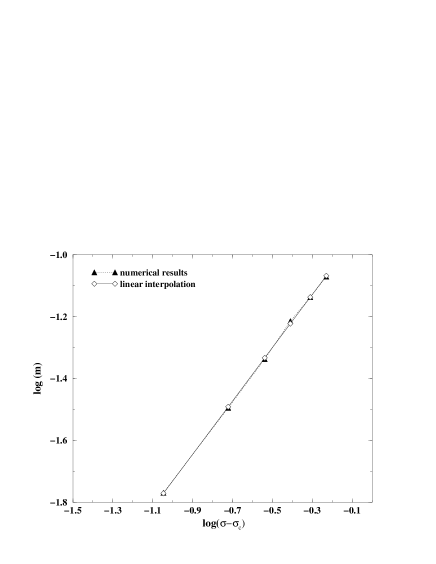
FIG. 3.: Order parameter $m$ as a function of $(\sigma-{\sigma}_{c})$ (on a log-log scale) in $d=1$. The slope gives the critical index ${\beta}_{\sigma}=0.9\pm 0.1$.

In order to determine the exponent $\beta_{a}$, defined as $m\propto{({a}_{c}-a)}^{{\beta}_{a}}$, we fix $\sigma=\sigma_{c}$, and diminish $a$ to stay in the active phase. Then we follow a maximization of the linear correlation coefficient procedure similar to the one described above. In that way we measure ${a}_{c}=1.04\pm 0.01$ and ${\beta}_{a}=1.5\pm 0.1$.

Right at the critical point the order parameter decays in time as $m(t)\propto t^{-\theta}$. In order to have an independent estimation of the critical point we plot the local slope of the averaged magnetization as a function of $1/t$ for different values of $\sigma$ (see Fig.(4)). It is clear that the curve for $\sigma=1.8$ ($\sigma=1.7$) curves upward (downward) and corresponds to the active (absorbing) phase; the critical point is located around $\sigma_{c}\approx 1.75$, slightly smaller than the previously determined value, but compatible with that value within accuracy limits. The intersection point at $1/t=0$ of the central curve gives the value of the exponent $\theta$; $\theta=1.1\pm 0.1$.

FIG. 4.: Local slope, $\theta(t)$, of $\log m(t)$ as a function of $\log t$, plotted as a function of $t^{-1}$. The extrapolated value at $t^{-1}=0$ gives the value of $\theta$, $\theta=1.1\pm 0.1$.

In order to measure spreading exponents we consider much larger system sizes. Simulations are stopped either when the activity arrives to any of the system boundaries. In this way we have determined $z^{\prime}$, $\eta$. Using the previously obtained valued $\sigma_{c}=1.75$, we measure $z^{\prime}=1.25\pm 0.10$ e $\eta=-0.4\pm 0.1$. The standard critical exponent $z$ is $z=\frac{2}{z^{\prime}}=1.6\pm 0.1$ compatible with the KPZ value $z=1.5$ (in an analogous discrete model argued to be in the same MN universality class, which is expected to converge faster to its asymptotic behavior we measured $z=1.52\pm 0.03$ [19], which remains the most accurate estimate for $z$). For this system the exponent $\nu_{x}$ has been already measured numerically [17, 19]; the result $\nu_{x}=1$ is in agreement with the theoretical prediction [16]. See Table I, for a complete list of the to the date best exponent estimates [17, 19, 14]. Observe that all the scaling relations (including that for spreading exponents) are satisfied within numerical accuracy.

B $d=2$

We have performed simulations in $d=2$ systems with $L^{2}=1600$, and confirmed the presence of a phase transition (as it was already observed in [14]), but have not performed extensive analysis to determine accurately the critical exponents. At $d=2$ there are two fixed points of the RG for KPZ a trivial, unstable, one at zero noise amplitude to which correspond, obviously, mean field exponents, and a stable, rough phase one, with non trivial exponents for any non-vanishing noise amplitude. Instead of analyzing this case with only one stable fixed point, we preferred to analyze the a priori more interesting three-dimensional case.

C $d=3$

In the three-dimensional simulations we consider system sizes up to $L^{3}=64000$ and periodic boundary conditions. The space and time meshes are $1$ and $0.001$ respectively. The spatial coupling constant is $D=1$.

1 The weak noise phase.

We fix $a=1$ for this small value we expect the transition to occur at a small value of $\sigma$, and therefore to be controlled by the weak noise fixed point (weak coupling, in he language of KPZ). In the weak noise regime the mean field predictions (see appendix) are expected to be exact, and therefore for $a=1$ one should have $1-\sigma^{2}/2=0$, implying $\sigma_{c}=\sqrt{2}$. In fact, following the same procedure described in the one-dimensional case, the best estimation of the critical point is ${\sigma}_{c}=1.420\pm 0.002$ (the deviation from $\sigma_{c}=\sqrt{2}$ is a finite size effect) and the slope of a log-log plot of the order parameter versus $\sigma-\sigma_{c}$ gives ${\beta}_{\sigma}=1.00\pm 0.01$ (see Fig. (5)).

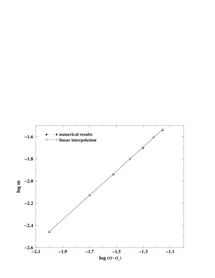
FIG. 5.: Order parameter $m$ as a function of $(\sigma-{\sigma}_{c})$ (on a log-log scale) in $d=3$ with $a=1$ and $p=2$. The slope gives the critical index ${\beta}_{\sigma}=1.00\pm 0.01$.

The order parameter time-decay exponent, $\theta$ is found to be $\theta=1.0\pm 0.1$, while for $z^{\prime}$ and $\eta$ we measure $z^{\prime}=1.00\pm 0.01$ (see Fig. ( 6)) and $\eta=-0.1\pm 0.1$. Using scaling relations we estimate $\nu_{x}=0.50\pm 0.05$.

FIG. 6.: Log-log plot of $R^{2}(t)$ as a function of $t$ at the critical point for $d=3$ and $a=1$. From the slope we obtain $z^{\prime}=1.00\pm 0.01$.

Fixing $\sigma=1.418$ we have measured $m$ for different values of $a$, with $a<1$. The linear correlation coefficient of a log-log plot of the order parameter versus $a-a_{c}$ is maximum for $a_{c}=0.995\pm 0.010$, and the corresponding slope gives ${\beta}_{a}=0.97\pm 0.05$, also compatible with its mean field value ${\beta}_{a}=1$ (see Fig. (7)).

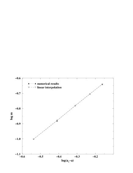
FIG. 7.: $\log(m)$ as a function of $\log({a}_{c}-a)$ and its corresponding linear interpolation for $a=1$, $\sigma=1.418$ and $d=3$. From the slope we measure ${\beta}_{a}=0.97\pm 0.05$.

Therefore, summing up, all the exponent in the weak noise regime are in good agreement with their corresponding mean field values, and their expected scaling relations are satisfied.

2 The strong noise phase.

Now we take a large value of $a$, namely $a=18$, for which the transition is expected to occur at a large value of the noise amplitude, and therefore to be controlled by a strong noise fixed point (strong coupling, in the KPZ language). We find the critical point to be located at ${\sigma}_{c}=7.2\pm 0.3$, and ${\beta}_{\sigma}=1.2\pm 0.1$ (see Fig. (8)). Observe that contrarily to the weak noise case, now the critical value of $\sigma$ is renormalized; the mean field prediction is $\sigma_{c}=\sqrt{2a}=6$.

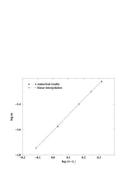
FIG. 8.: Log-log plot of the stationary value of the order parameter $m$ as a function of $\sigma-\sigma_{c}$ for $a=18$ and $d=3$. From the slope we measure ${\beta}_{\sigma}=1.2\pm 0.1$ .

Following the previously described methods, we we obtain $\theta=2.0\pm 0.1$, and for the spreading exponents $z^{\prime}=1.20\pm 0.01$, and $\eta=-0.5\pm 0.1$ (the best power laws fit for the spreading exponents are obtained for $\sigma=6.875$ slightly smaller that the critical value obtained from the order parameter analysis). Using the value of $z^{\prime}$, we obtain $z=\frac{2}{z^{\prime}}=1.67\pm 0.03$ in excellent agreement with the best estimation for the strong noise phase of KPZ in $d=3$, namely $z=1.695$ [34]. And applying the scaling law relating $z$ and $\nu_{x}$, we obtain. $\nu_{x}=0.75\pm 0.03$. On the other hand the hyperscaling relation for spreading exponents Eq. (16) is not expected to hold above the upper critical dimension where dangerously irrelevant operators should affect it [31] and, in fact, introducing the values obtained numerically one observes that it is clearly violated.

Fixing $\sigma$ to its critical value and varying $a$ we obtain ${\beta}_{a}=2.5\pm 0.1$ (see Fig. (9)); in particular, ${\beta}_{a}\geq 1$ in agreement with the prediction made in [16]. Contrarily to the mean field predictions observe that in the strong noise regime $\beta_{a}\neq\beta_{\sigma}$.

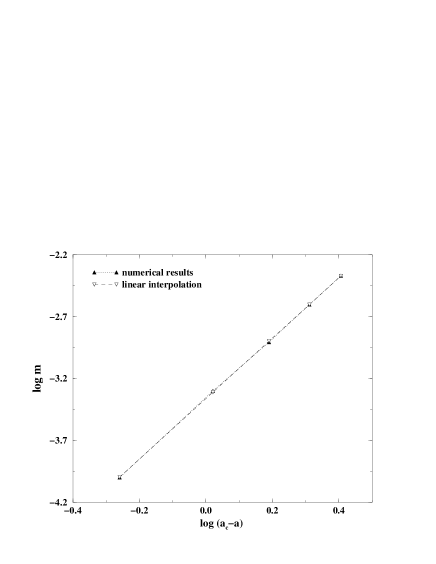
FIG. 9.: $\log(m)$ as a function of $\log({a}_{c}-a)$ and its corresponding linear interpolation for $\sigma=6.875$ and ${a}_{c}=18.05$, for $d=3$. From the slope we determine ${\beta}_{a}=2.5\pm 0.1$.

Using $\nu_{x}=\beta_{a}/(z\theta)$ and introducing the measured values of $\beta_{a}$, $\theta$, and $z$, we determine $\nu_{x}=0.76\pm 0.03$ in excellent agreement with our previous estimation. This provides a test for the accuracy of our measurements.

In conclusion, we have verified numerically the existence of two different regimes for the MN equation exhibiting different values of the critical exponents, and related respectively to the weak and strong coupling regimes of the KPZ equation.

V Ito-Stratonovich dilemma

In order to study the dependence of the NIOT on the type of interpretation, in the sense of the Ito-Stratonovich dilemma, of the Langevin equation let us now consider Eq. (3) intended in the Ito sense. It is obvious that an equation completely equivalent to Eq.(3), i.e. with exactly the same physics, can be written in the Ito interpretation using the well known transformation rules [35, 36]. The problem we study here is different; we analyze the same multiplicative noise Langevin equation in a different interpretation, i.e. Ito instead of Stratonovich.

By repeating the mean field like approximations discussed in the appendix, but using the Ito interpretation, one obtains the same final results Eq. (26), and (44) just by substituting $(\sigma^{2}/2-a)$ by $-a$. Therefore for positive definite initial conditions, and positive values of $a$ (i.e. values for which the deterministic equation has $m=0$ as the only solution), there is no non-trivial solution. This indicates that the NIOT disappears when intending the MN in the Ito sense, and therefore, in the Stratonovich interpretation it is due to the effective shift of the a-dependent term in the stationary probability distribution when multiplicative noise is introduced. In the same way, it is also straightforward to verify by performing a linear stability analysis that the homogeneous solution $\psi=0$ is stable, contrarily to what happens in the Stratonovich interpretation. The presence of an instability had been identified as a key ingredient to generate noise induced transitions (see [14] and references therein), and therefore in absence of it no ordering is expected in the Ito interpretation.

We have verified this prediction in numerical simulations.

VI Coupling constant dependence

In this section we pose ourselves the question of which is the minimum value of the coupling necessary to obtain a NIOT. As pointed out in [10, 5] the NIOT appears due to the interplay between a short time instability and the presence of a spatial coupling that renders stable the generated non trivial state. In all the previously discussed models exhibiting a NIOT and a NIDT there are critical values of $D$ below which no ordering is possible. In order to determine whether there is a critical $D$ in our model we have studied it in $d=1$ by changing $D$ with fixed $a=1$ (the forthcoming results are qualitatively independent of the value of $a$). In Fig. (10) we show a sketchy phase diagram, outcome of systematic numerical simulations.

FIG. 10.: Schematic Phase diagram in the plane $(\sigma,D)$ for the MN Langevin equation. The rightmost line of second order phase transitions moves to the right as $\alpha$ is reduced; and goes to $\infty$ in the limit $\alpha=0$, indicating that the NIDT disappears.

There is a large interval of values of $\sigma$ for which the system exhibits a first order transition at $D=0$; i.e. as soon as an arbitrarily small spatial coupling is switched on the system gets ordered (for $D=0$ the only stationary state is $m=0$). In Fig. (11) the order parameter is plotted as a function of $1/D$ for a value of $\sigma$ in this interval; observe how even for values as small as $D=10^{-7}$, $m$ takes a large value of about $0.15$.

FIG. 11.: Order parameter $m$ as a function of $1/D$ for $\sigma=10$ and $a=1$. The curve converges to a constant for large values of $1/D$, this is for small couplings, indicating that at $D=0$ there is a first order phase transition.

The fact that there is a large interval for which the systems becomes ordered as soon as a spatial coupling is switched on, property that was absent in all the previously studied models for NIOT, is a new indication that the MN equation is the minimal model for NIOT, and that the associated ordering mechanism is not mixed up with other unnecessary ingredients.

For values of $\sigma$ out of the previously discussed interval, the system exhibits a second order phase transitions at a value of $D$, $D_{c}(\sigma)$, Defining $\beta_{D}$ by

$$m\propto{\left(D-{D}_{c}\right)}^{{\beta}_{D}},$$ (23)

we obtain ${D}_{c}=0.094\pm 0.003$ and ${\beta}_{D}=0.08\pm 0.03$ for the particular choice of parameters $a=\sigma=5$.

VII Conclusions

We have presented some recent results on Langevin equations with multiplicative noise. In particular, we have studied numerically for the first time the presence of two different regimes: Weak and a strong noise regimes, in $d=3$. All the predicted scaling laws and relations with KPZ exponents in its respective weak coupling and strong coupling fixed points are verified. On he other hand, we have shown that the noise induced ordering transition associated with Langevin equations with multiplicative noise is specific of the Stratonovich representation, and shown that these noise induced ordering transitions are obtained even for arbitrarily small values of the spatial coupling constant, supporting the fact that the Langevin equation with pure multiplicative noise is the minimal model for noise induced ordering transitions.

VIII Appendix

In this appendix we present some different mean field approximations to evaluate the order parameter exponent for both $\alpha=0$ and $\alpha>0$.

Defining the averaged magnetization as $m$, in the limit of large dimensionalities the discretized Laplacian operator can be written as

$$\nabla^{2}\psi=1/2d\sum_{j,N.N.}\psi_{j}-\psi_{i}\approx m-\psi_{i}.$$ (24)

Using this approximation, and determining $m$ in a self-consistent way it is possible to obtain an analytical solution of the Langevin equation. In what follows we present different calculations corresponding to infinite and finite values of the spatial coupling $D$ respectively. In both cases the obtained value of the critical exponent $\beta_{a}$ is $1/p$.

A Infinite spatial coupling limit: $D\rightarrow\infty$

Using the previous approximation, writing down the stationary probability distribution, solution of the associated Fokker-Planck equation [35, 36], and imposing the self-consistent requirement $m=<\psi>$ we obtain

$${m=\frac{\int_{I}d\psi\psi\exp\int_{0}^{\psi}d\psi\frac{F+D(m-\psi)-GG^{\prime}/2}{G^{2}/2}}{\int_{I}d\psi\exp\int_{0}^{\psi}d\psi\frac{F+D(m-\psi)-GG^{\prime}/2}{G^{2}/2}}}.$$ (25)

For large values of $D$ the integral can be evaluated in saddle point approximation [5, 10], giving

$$m={\left[\frac{1}{p}\left(\frac{{\sigma}^{2}}{2}-a\right)\right]}^{\frac{1}{p}}.$$ (26)

The NIOT transition is predicted at $\frac{{\sigma}^{2}}{2}=a$ with an associated exponent ${\beta}_{a}={\beta}_{\sigma}=\frac{1}{p}$.

B Finite spatial coupling

In order to make sure that the previous result is not due to the approximation involved in considering $D\rightarrow\infty$, we present here an analogous calculation for finite values of $D$. In this case, the associated asymptotic stationary probability is

$$P_{\infty}\propto{\psi}^{-1-\frac{2}{{\sigma}^{2}}(a+D)}\exp{\left(-\frac{2Dm}{{\sigma}^{2}\psi}\right)}\exp{\left(-\frac{2}{{\sigma}^{2}}{\psi}^{p}\right)}$$ (27)

where $m$ has to be fixed self-consistently by imposing $m=\langle\psi\rangle$, this is

$${m=\frac{\int_{0}^{\infty}d\psi{\psi}^{-\frac{2(a+D)}{{\sigma}^{2}}}\exp\left(-\frac{2Dm}{{\sigma}^{2}\psi}-\frac{2}{{\sigma}^{2}}{\psi}^{p}\right)}{\int_{0}^{\infty}d\psi{\psi}^{-1-\frac{2(a+D)}{{\sigma}^{2}}}\exp\left(-\frac{2Dm}{{\sigma}^{2}\psi}-\frac{2}{{\sigma}^{2}}{\psi}^{p}\right)}.}$$ (28)

The numerical solution of this last equation for parameter values $a=1,D=1$, and $p=1$ is shown in Fig. 12 and Fig. 13.

FIG. 12.: The solution, $m$, of the self-consistency equation is the intersection point between $y=f(m)$ (where $f(m)$ represents the function on the r.h.s. of Eq. ()) and $y=m$.

FIG. 13.: $m$ as a function of $\sigma$ in mean field theory with $\alpha=0$. The points here correspond to the intersection of the curves in the previous figure with the line $m=f(m)$. The critical point is located at $\sigma_{c}^{2}=2$.

In order to derive the exponent $\beta_{a}$ in this MF approximation we define the following change of variables,

$$t = \frac{1}{\psi}$$ (29)

$$\alpha = \frac{2}{{\sigma}^{2}}$$ (30)

$$\gamma = \frac{2}{{\sigma}^{2}}(a+D)$$ (31)

$$\mu = \frac{2Dm}{{\sigma}^{2}}.$$ (32)

Eq. (28) can be written as

$${\frac{\mu}{\alpha D}=-1/{\partial}_{\mu}\log{\left\{\int_{0}^{\infty}dt\ {t}^{\gamma-2}\exp\left[-\mu t-\frac{\alpha}{{t}^{p}}\right]\right\}}.}$$ (33)

Introducing a Gaussian transformation the integral in the previous expression can be rewritten as

$$\int_{0}^{\infty}dt\ {t}^{\gamma-2+\frac{p}{2}}\exp[-\mu t]\int_{-\infty}^{+\infty}d\eta\ \exp\left[-\frac{{t}^{p}{\eta}^{2}}{4\alpha}+i\eta\right]=$$ (34)

$$\ \ \ \ \ \ ={\mu}^{1-\gamma}\int_{-\infty}^{+\infty}d\eta\ \exp\left(i\eta\sqrt{4\alpha{\mu}^{p}}\right)$$ (35)

$$\ \ \ \ \ \ \ \ \ \ \ \ \ \ \ \ \ \ \ \ \ \int_{0}^{\infty}\frac{dt}{t}\ {t}^{\gamma+\frac{p}{2}-1}\exp\{-t-{t}^{p}{\eta}^{2}\}=$$ (36)

$$\ \ \ \ \ \ ={\mu}^{1-\gamma}\int_{0}^{\infty}d\eta\cos\left(\eta\sqrt{4\alpha{\mu}^{p}}\right)$$ (37)

$$\ \ \ \ \ \ \ \ \ \ \ \ \ \ \ \ \ \ \ \ \int_{0}^{\infty}\frac{dt}{t}\ {t}^{\gamma+\frac{p}{2}-1}\exp\{-t-{t}^{p}{\eta}^{2}\}=$$ (38)

$$={\mu}^{1-\gamma}\{{H_{0}}^{(p)}(\gamma+\frac{p}{2}-1)-2\alpha{\mu}^{p}{H_{1}}^{(p)}(\gamma+\frac{p}{2}-1)+...\}$$ (39)

(40)

where we have expanded the cosine function up to second order, and we have defined

$${H_{n}}^{(p)}(\delta) = \int_{0}^{\infty}\ {\eta}^{2n}{\Gamma}_{p}(\delta,{\eta}^{2})$$ (41)

$${\Gamma}_{p}(\delta,{\eta}^{2}) = \int_{0}^{\infty}\frac{dt}{t}{t}^{\delta}\exp{\{-t-{t}^{p}{\eta}^{2}\}}$$ (42)

for $\delta>0$. This calculation is valid only if $\gamma+\frac{p}{2}>1$. At the end of the calculation we will verify that this constraint is verified. Eq. (33) can be simply expressed as

$$\alpha D=2\alpha p{{H_{1}}^{(p)}(\gamma+\frac{p}{2}-1)\over{H_{0}}^{(p)}(\gamma+\frac{p}{2}-1){\mu}^{p}}+(\gamma-1).$$ (43)

From this we find the solution $\mu=0$ corresponding to $m=0$ and if $\frac{{\sigma}^{2}}{2}-a\geq 0$ a second solution exists with

$$m=\frac{{\sigma}^{2}}{2D}{\left(\frac{{H_{0}}^{(p)}}{2{H_{1}}^{(p)}}\right)}^{\frac{1}{p}}{\left[\frac{1}{p}\left(\frac{{\sigma}^{2}}{2}-a\right)\right]}^{\frac{1}{p}}\propto{\left(\frac{{\sigma}^{2}}{2}-a\right)}^{\frac{1}{p}}.$$ (44)

This solution confirms the results obtained in the $D\rightarrow\infty$ case; namely ${a}_{c}=\frac{{\sigma}^{2}}{2}$, for $a\geq 0$, ${{\sigma}_{c}}^{2}=2a$, and ${\beta}_{\sigma}={\beta}_{a}=\frac{1}{p}$ which is consistent with the requirement $\gamma+p/2>0$ for all the values of $p$ rendering consistent the calculation.

C Infinite coupling limit for $\alpha>0$

For completeness’ sake let us present here the mean field analysis in the case in which $\alpha>0$. In this subsection we evaluate the infinite coupling limit.

The solution $m=0$ is unstable for ${\sigma}^{2}>2a$, and the new stable solution is

$$m={\left[\frac{{\sigma}^{2}-2a}{(p)({\sigma}^{2}+1)}\right]}^{\frac{1}{p}}.$$ (45)

Let us notice that this approximation predicts a NIOT at the same point the pure MN equation (with $\alpha=0$) does, namely $\sigma^{2}=a/2$, but contrarily to the pure model the order parameter does not grow indefinitely by increasing noise amplitude. Instead it saturates to a value $m=(p)^{-1/p}$.

D Finite coupling for $\alpha>0$

In the case of finite coupling $D$ and $\alpha>0$ we have that the asymptotic probability defined in the interval $0\leq\psi\leq 1$ is (for $p=1$)

$$P_{\infty}(\psi)\propto{\psi}^{-\left(1+\frac{2(a+D)}{{\sigma}^{2}}\right)}{\left(\frac{1-\psi}{1+\psi}\right)}^{-\frac{Dm}{{\sigma}^{2}}}$$ (46)

$$\ \ \ \ \ \ \ \ \ \ \ \ \ \ \ \ {(1-{\psi}^{2})}^{-\frac{1}{2}+\frac{a+D+1}{{\sigma}^{2}}}\exp\left[-\frac{2Dm}{{\sigma}^{2}\psi}\right].$$ (47)

The self-consistency equation is obtained equating $m$ to

$${\frac{\int_{0}^{1}d\psi\ {\psi}^{-\frac{2(a+D)}{{\sigma}^{2}}}{(\frac{1-\psi}{1+\psi})}^{-\frac{Dm}{{\sigma}^{2}}}{(1-{\psi}^{2})}^{-\frac{1}{2}+\frac{a+D+1}{{\sigma}^{2}}}e^{-\frac{2Dm}{{\sigma}^{2}\psi}}}{\int_{0}^{1}{\psi}^{-(1+\frac{2(a+D)}{{\sigma}^{2}})}{(\frac{1-\psi}{1+\psi})}^{-\frac{Dm}{{\sigma}^{2}}}{(1-{\psi}^{2})}^{-\frac{1}{2}+\frac{a+D+1}{{\sigma}^{2}}}e^{-\frac{2Dm}{{\sigma}^{2}\psi}}}.}$$ (48)

Both of the integrals exhibit a singularity at $\psi=1$, but they are integrable. It is straightforward verifying that in the limit $\sigma\rightarrow\infty$, $m\rightarrow 0$, and therefore for finite values of $D$ this approximation predicts both a NIOT (also located at $\sigma^{2}=2a$) and a NIDT.

FIG. 14.: Solution of the mean field theory for $\alpha>0$. Observe that contrarily to what happens in Fig. 13, here the intersection point between the curves for different values of $\sigma$ and the straight line $y=m$ reaches a maximum value after which it starts decreasing.

FIG. 15.: $m$ as a function of $\sigma$ in mean field theory with $\alpha>0$. The points here correspond to the intersection of the curves in the previous figure with the line $m=f(m)$. The critical point is located at $\sigma_{c}^{2}=2$.

ACKNOWLEDGEMENTS

We acknowledge useful discussions with P. Garrido, G. Grinstein, Y. Tu, T. Hwa, J. M. Sancho, L. Pietronero, R. Dickman, G. Parisi and R. Toral. We thank Claudio Castellano and R. Pastor-Satorras for a critical reading of the manuscript. M.A.M. is supported by the M. Curie fellowship contract ERBFMBICT960925, and by the TMR ’Fractals’ network, project number EMRXCT980183.

d	$1$	$3\ (WeakN.)$	$3\ (StrongN.)$
${\beta}_{a}$	$1.5\pm 0.1$	$0.97\pm 0.05$	$2.5\pm 0.1$
${\beta}_{\sigma}$	$0.9\pm 0.1$	$1.0\pm 0.01$	$1.2\pm 0.1$
$z$	$1.52\pm 0.03$	$2.00\pm 0.05$	$1.67\pm 0.03$
$\eta$	$-0.4\pm 0.1$	$-0.1\pm 0.05$	$-0.5\pm 0.1$
$\theta$	$1.1\pm 0.1$	$1.0\pm 0.1$	$2.0\pm 0.1$
$\nu_{x}$	$1.0\pm 0.1$	$0.50\pm 0.05$	$0.75\pm 0.03$

TABLE I.: Table of critical indices obtained from numerical simulations. In the second column we report results for the $d=1$ case. In the three-dimensional weak noise phase (third column) the exponents are in very good agreement with the expected mean field values. The last column reports the numerical values obtained in his work for the three-dimensional exponents in the strong noise phase.

REFERENCES

- [1] R. Benzi, A. Sutera and A. Vulpiani, J. Phys. A 14, L453 (1981). K. Weisenfeld and F. Moss, Nature 373, 33 (1995)
- [2] C. R. Doering and J. C. Gadoua, Phys. Rev. Lett. 69, 2318 (1992). See also, P. Pechukas and P. Hänggi, Phys. Rev. Lett. 73, 2772 (1994).
- [3] J. García-Ojalvo, A. Hernández-Machado and J. M. Sancho, Phys. Rev. Lett. 71, 1542 (1993); J. M. Parrondo, C. Van den Broeck, J. Buceta and F. J. de la Rubia, Physica A 224, 153 (1996).
- [4] S. Kim, S. H. Park, and C. S. Ryu, Phys. Rev. Lett. 78, 1616 (1997).
- [5] C. Van den Broeck, J. M. R. Parrondo and R. Toral, Phys. Rev. Lett. 73, 3395 (1994).
- [6] A. Becker and L. Kramer, Phys. Rev. Lett. 73, 955 (1994).
- [7] C. Van den Broeck, J.M.R. Parrondo, J. Armero and A. Hernández-Machado, Phys. Rev. E 49, 2639 (1994).
- [8] W. Genovese, M. A. Muñoz and P.L. Garrido, Phys. Rev. E 58, 6828 (1998).
- [9] See W. Horsthemke e R. Lefever, Noise Induced Transitions, Springer Verlag, Berlin, 1984, and references therein.
- [10] C. Van den Broeck, J. M. R. Parrondo, R. Toral and R. Kawai, Phys. Rev. E 55, 4084 (1997).
- [11] J. García-Ojalvo, J. M. R. Parrondo, J.M. Sancho and C. Van den Broeck, Phys. Rev. E 54, 6918 (1996).
- [12] S. Kim, S. H. Park and C. S. Ryu, Phys. Rev. Lett. 78, 1616 (1997).
- [13] R. Müller, K. Lippert, A. Kühnel and U. Behn, Phys. Rev. E 56, 2658 (1997).
- [14] W. Genovese, M.A. Muñoz and J. M. Sancho, Phys. Rev. E 57, R2495 (1998).
- [15] S. Kim, S. H. Park and C. S. Ryu, Phys. Rev. Lett. 78, 1827 (1997).
- [16] G. Grinstein, M.A. Muñoz and Y. Tu, Phys. Rev. Lett. 76, 4376 (1996).
- [17] Y. Tu, G. Grinstein and M.A. Muñoz, Phys. Rev. Lett. 78, 274 (1997).
- [18] M. Kardar, G. Parisi and Y. C. Zhang, Phys. Rev. Lett. 56, 889 (1986).
- [19] M.A. Muñoz and T. Hwa, Europhys. Lett. 41, 147 (1998).
- [20] H. Hinrichsen, R. Livi, D. Mukamel and A. Politi, Phys. Rev. Lett. 79, 2710 (1997).
- [21] E. Medina, T. Hwa and M. Kardar, Phys. Rev. A 39, 3053 (1989). M. Lässig Nucl. Phys. B 448, 559 (1995).
- [22] T. Halpin-Healy and Y.-C. Zhang, Phys. Rep. 254, 215 (1995).
- [23] A. L. Barabási, H. E. Stanley, Fractal Concepts in Surface Growth Cambridge University Press, Cambridge, 1995.
- [24] In the case there are two different walls: the one discussed in the text, and another one at a smaller value, at . As goes to this second wall goes to . By performing a change of variables , and , the Langevin equation for , has a noise amplitude proportional to . Even if the noise amplitude is proportional to the square root of the field, the critical phenomena associated at this NIDT are not expected to be related to the Reggeon field theory (RFT) and directed percolation [25]. This is because this second wall, in spite of having a RFT like noise is not truly absorbing, i.e. the dynamics does not cease even for a flat configuration at .
- [25] See for example, G. Grinstein and M. A. Muñoz, in Fourth Granada Lectures in Computational Physics, Ed. P. Garrido and J. Marro, Springer (Berlin) 1997. Lecture Notes in Physics, 493, 223 (1997), and references therein.
- [26] P. Grassberger and A. De La Torre, Ann. Phys. 122, 373 (1979)
- [27] M. A. Muñoz, G. Grinstein and Y. Tu, Phys. Rev. E 56, 5101 (1997).
- [28] J.F.F. Mendes, R. Dickman, M. Henkel and M.C. Marques, J. Phys. A 27, 3019 (1994).
- [29] C. Castellano, M. Marsili and L. Pietronero, Phys. Rev. Lett. 80, 4830 (1998). C. Castellano, A. Gabrielli, M. Marsili, M. A. Muñoz, and L. Pietronero. E 58, R5209 (1998).
- [30] C. J. DeDominicis, J. Physique 37, 247 (1976); H.K. Janssen, Z. Phys. B 23, 377 (1976); P. C. Martin, E. D. Siggia and H. A. Rose, Phys. Rev. A 8, 423 (1978); L. Peliti, J. Physique, 46, 1469 (1985).
- [31] J. Zinn-Justin, Quantum Field Theory and Critical Phenomena (Oxford Science, Oxford, 1989).
- [32] Schenzle and H. Brand, Phys. Rev. A 20, 1628 (1979). R. Graham and A. Schenzle, Phys. Rev. A 25, 1731 (1982).
- [33] M. San Miguel and R. Toral, Stochastic Effects in Physical Systems, to be published in Instabilities and Nonequilibrium Structures, VI, E. Tirapegui and W. Zeller, eds. Kluwer Academic Pub. (1997). (Cond-mat/9707147).
- [34] T. Ala-Nissila, Phys. Rev. Lett. 80, 887 (1998).
- [35] N.G. van Kampen, Stochastic Processes in Physics and Chemistry, North Holland, Amsterdam, 1981.
- [36] C. W. Gardiner, Handbook of Stochastic Methods, Springer Verlag, Berlin and Heidelberg, 1985.