Chaos in Quantum Dots: Dynamical Modulation of Coulomb Blockade Peak Heights

Abstract

We develop a semiclassical theory of Coulomb blockade peak heights in quantum dots and show that the dynamics in the dot leads to a large modulation of the peak height. The corrections to the standard statistical theory of peak height distributions, power spectra, and correlation functions are non-universal and can be expressed in terms of the classical periodic orbits of the dot that are well coupled to the leads. The resulting correlation function oscillates as a function of peak number in a way defined by such orbits; in addition, the correlation of adjacent conductance peaks is enhanced. Both of these effects are in agreement with recent experiments.

The electrostatic energy of an additional electron on a quantum dot– a mesoscopic island of confined charge with quantized states– blocks the flow of current through the dot, an effect known as the Coulomb blockade[1]. Current can flow only if two different charge states of the quantum dot are tuned to have the same energy; this produces a peak in the the conductance of the dot whose magnitude is directly related to the magnitude of the wavefunction near the contacts to the dot. Since dots are generally irregular in shape, the dynamics of the electrons is chaotic, and the characteristics of Coulomb blockade peaks reflect those of wavefunctions in chaotic systems[2, 3, 4]. Previously, a statistical theory for the peaks was derived[2, 3] by assuming these wavefunctions to be completely random and uncorrelated with each other. The experimental data[5, 6] for the distribution of the Coulomb blockade peak heights were found to be in excellent agreement with the predictions of the statistical theory, thus giving a solid foundation to the conjecture of effective “randomness” of the quantum dot wavefunctions.

It therefore came as a surprise when several recent experiments[6, 7, 8] demonstrated large correlations between the heights of adjacent peaks. The effect of nonzero temperature (when several resonances contribute to the same peak) was found to be insufficient to account for these correlations[9]. To explain the correlations, the enhancement due to spin-paired levels[8, 9], due to a decrease of the effective level spacing found in density functional calculations[10], and due to of level anticrossings in interacting many-particle systems[11] were proposed. However, we show here that peak height correlations arise already within an effective single-particle picture of the electrons in the quantum dot. The specific internal dynamics of the dot, even though it is chaotic, modulates the peaks: because all systems have short-time features, chaos is not equivalent to randomness. The predicted dynamical modulation is exactly of the type needed to explain the experiments[6, 7, 8].

To study the non-universal effects of the dynamics of a particular dot, we derive a relation between the quantum conductance peak height and the classical periodic orbits in the dot. The main effect is that as a system parameter varies– the magnetic field or the number of electrons in the dot in response to a gate voltage, for instance– the interference around each periodic orbit oscillates between being destructive and constructive. When the interference is constructive for those periodic orbits which come close to the leads used to contact the dot, the wavefunction is enhanced near the leads, the dot-lead coupling is stronger, and so the conductance is larger. Likewise, destructive interference produces a smaller conductance. The resulting modulation can be substantial, as shown in Fig. 1. Similar short-time dynamical effects have been noted in other contexts such as atomic and molecular spectra[12, 13, 14], eigenfunction scarring[14, 15], magnetotransport in antidot lattices[16], and tunneling into quantum wells[17, 18, 19]. Such modulation is completely omitted in theories in which the wavefunction is assumed to change randomly as the system changes[2, 3].

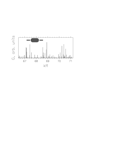
FIG. 1.: The peak conductance from tunneling through subsequent energy levels for the stadium billiard shown in the inset. Each peak is placed at the wavevector $k$ corresponding to its level; $R$ is the radius of the half-circle parts of the stadium. A Gaussian lead wavefunction appropriate for tunneling from a single transverse mode is used with width $ka_{\rm eff}=15$.

Our starting point is the connection between the peak height and the width of the level in the quantum dot. We consider a dot close to two leads (Fig. 1 inset) so that the width, $\Gamma$, of a level comes from tunneling of the electron to either lead. When the mean separation of levels is larger than the temperature $T$ which itself is much larger than the mean width, the electrons pass through a single quantized level in the dot. The conductance peak height in this regime is[20]

$$G_{\rm peak} = \frac{e^{2}}{h}\frac{\pi{\Gamma}}{4kT}.$$ (1)

Here for simplicity we consider symmetrically placed leads– the total width is equally split between tunneling to the right and left leads– spinless particles, and temperature much smaller than the level spacing.

The width of the level is related by Fermi’s Golden Rule to the square of the matrix element for tunneling between the lead and the dot, $M^{\ell\rightarrow d}$. A convenient expression for the matrix element in terms of the lead and dot wavefunctions, $\Psi_{\ell}$ and $\Psi_{d}$ respectively, was derived by Bardeen[21] and can be expressed as[17, 18]

$$M^{\ell\rightarrow d}=\frac{\hbar^{2}}{m^{*}}\int_{S}d{\bf S}\Psi_{\ell}(r){\bf\bigtriangledown}\Psi_{d}(r)$$ (2)

where the surface $S$ is the edge of the quantum dot. $\Gamma$, then, depends on the square of the normal derivative of the dot wavefunction at the edge weighted by the lead wavefunction. Writing the product of the two $\Psi_{d}$’s in $\Gamma$ as a Green function $G(r,r^{\prime})$ and using the standard semiclassical expression for the latter[12], we express $\Gamma$ as a sum over the classical trajectories which start at $r$ on the edge of the dot near the lead and end at $r^{\prime}$ which is also on the edge near the lead.

Tunneling from the lead to the dot is dominated by the lowest transverse energy subband in the constriction between the lead and the dot[3]. Therefore, for the calculation of the tunneling matrix element the transverse potential in the tunneling region can be taken quadratic: $U_{\ell}\sim\kappa\left(y-y_{\ell}\right)^{2}$. In this case the transverse dependence of the lead wavefunction is simply a harmonic oscillator wavefunction, so that at the edge of the dot $\Psi_{\ell}\sim c_{\ell}\exp[-(y-y_{\ell})^{2}/2a_{\rm eff}^{2}]$, where $\hat{\bf y}$ represents the direction tangential to the boundary of the dot, $y_{\ell}$ is the center of the lead and constriction, and the effective width is $a_{\rm eff}=\sqrt{\hbar}/\sqrt[4]{2\kappa m^{*}}$. While the exact form of the lead wavefunction is not crucial, the $\hbar$-dependence of the width is important for the semiclassical argument which follows; note that $a_{\rm eff}\sim\sqrt{\hbar}$ does not depend on a particular transverse potential.

Using this information about $\Psi_{\ell}$ in the expression for $M^{\ell\rightarrow d}$, we see that the lead wavefunction restricts the integration to a semiclassically narrow region of width $a_{\rm eff}\sim\sqrt{\hbar}$. This allows one to express the contribution of the open trajectories entering the Green function in terms of an expansion near their closed neighbors. In the resulting expression for $\Gamma$, the contribution of each of these closed orbits is suppressed by a factor exponentially small in $\Delta p_{y}^{2}$, where $\Delta p_{y}$ is the change of transverse momentum after one traversal. This suppression is the effect of the mismatch of the closed orbit (momentum) with the distribution of transverse momentum at the lead, which is centered at zero with width $\delta p_{\ell}\sim\hbar/a_{\rm eff}\sim\sqrt{\hbar}$ for the lowest subband. Therefore, only closed orbits with semiclassically small momentum change $\Delta p$ contribute to the width. This in turn implies that the closed orbit is located semiclassically close (within a distance $\sim\sqrt{\hbar}$) to a periodic orbit for which $\Delta p\equiv 0$. Thus, one can express the tunneling width in terms of the properties of these periodic orbits, obtaining[22]

$$\Gamma=\bar{\Gamma}+\sum_{\mu:{\rm p.o.}}A_{\mu}\cos\left(\frac{S_{\mu}}{\hbar}+\phi_{\mu}\right)$$ (3)

where the monotonic part is

$$\bar{\Gamma}=\frac{\sqrt{\pi}}{2}c_{\ell}^{2}a_{\rm eff}\frac{p^{2}}{m^{*}}\ e^{-\zeta}\ \left[I_{0}\left(\zeta\right)+I_{1}\left(\zeta\right)\right],\ \ \zeta=\frac{p^{2}a_{\rm eff}^{2}}{2\hbar^{2}},$$ (4)

the amplitude is

$$A_{\mu} = 4\sqrt{2}\ \frac{\hbar c_{\ell}^{2}p^{\mu}_{z}}{m^{*}}\ \left[{\rm Tr}^{2}\left[M_{\mu}\right]\left(1+\sigma_{+}^{2}\right)\left(1+\sigma_{-}^{2}\right)\right]^{-1/4}$$ (5)

$$\times \exp\left(-\frac{\sigma_{+}^{2}\bar{p}^{2}}{\left(1+\sigma_{+}^{2}\right)}-\frac{\sigma_{-}^{2}\bar{y}^{2}}{\left(1+\sigma_{-}^{2}\right)}\right)$$ (6)

with

$$\sigma_{\pm} \equiv \frac{1}{2}\left[\overline{m}_{12}\!-\!\overline{m}_{21}\pm\sqrt{\left(\overline{m}_{22}\!-\!\overline{m}_{11}\right)^{2}+\left(\overline{m}_{21}\!+\!\overline{m}_{12}\right)^{2}}\right]$$ (7)

$$\overline{m}_{ij} \equiv \frac{2m^{\mu}_{ij}}{{\rm Tr}\left[M_{\mu}\right]+2}\left(\frac{a_{\rm eff}^{2}}{\hbar}\right)^{\frac{j-i}{2}}$$ (8)

$$\theta \equiv \frac{1}{2}\arctan\left(\frac{\overline{m}_{22}-\overline{m}_{11}}{\overline{m}_{21}+\overline{m}_{12}}\right)$$ (9)

$$\bar{y} \equiv \cos\theta\left(y_{\mu}-y_{\ell}\right)/a_{\rm eff}+\sin\theta\ p^{\mu}_{y}a_{\rm eff}/\hbar$$ (10)

$$\bar{p} \equiv \cos\theta\ p^{\mu}_{y}a_{\rm eff}/\hbar-\sin\theta\left(y_{\mu}-y_{\ell}\right)/a_{\rm eff}\,,$$ (11)

and, finally, the result for the slowly varying phase $\phi_{\mu}$ will be given elsewhere. Here $I_{n}$ is the Bessel function of complex argument, ${\bf p}^{\mu}$ is the electron momentum for the periodic orbit $\mu$ at the bounce point, $y_{\mu}$ is the bounce point coordinate, $S_{\mu}$ is the action of the periodic orbit, and $M_{\mu}\equiv\left(m_{ij}^{\mu}\right)$ is the corresponding monodromy matrix[12]. The semiclassical approach used here is similar to the calculation of the tunneling current in a resonant tunneling diode in a magnetic field developed in Ref. [17] and [19].

The equation above is the main result of this paper: it expresses the modulation of the heights of the Coulomb blockade peaks by the classical periodic orbits. Note that the result (3) is valid not only for chaotic but also for both integrable and mixed systems (for an integrable system or for the contributions of the remaining unbroken tori of a mixed system ${\rm Tr}\left[M\right]\equiv 2$).

In order to assess the validity of the semiclassical expression (3), we compare it to numerical calculations for two simple billiards, one integrable– the circle– and one chaotic– the stadium. The stadium billiard (Fig. 1 inset) is one of the canonical examples of a completely chaotic system[12]. From the dot wavefunctions (numerically obtained using the method of Ref. [23]), $\Gamma$ can be calculated from Eq. (2) using the $\Psi_{\ell}$ given above. To observe the variation in peak height, we vary the energy, or equivalently the wavevector $k\!\!=\!p/\hbar$, which changes the number of electrons on the dot as more levels are filled.

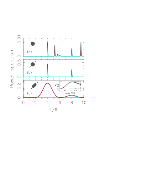
FIG. 2.: Length spectrum of the oscillations in $G(k)$ obtained from the Fourier power, numerical (blue) and semiclassical (red) results compared. The power is normalized to the mean conductance and then this mean is removed for clarity. (a) Circular dot with narrow leads, $ka_{\rm eff}\approx 1.2$. where $a_{\rm eff}$ is the width of the lead wavefunction. (b) Circular dot with wider leads, $ka_{\rm eff}\approx 12$. (c) Stadium dot using data in Fig. 1; dependence of amplitude at $L/R\!\!=\!4$ on $ka_{\rm eff}$ in inset. The width of the peaks reflects the length of $G(k)$ used. More data was available for the circle because it is integrable; conservation of angular momentum allows a simple representation of the wavefunctions in terms of Bessel functions. In (a) the peak at $L/R\!\!=\!4$ is the diameter, that at $8$ is its repetition, those accumulating to $2\pi$ are the whispering gallery trajectories, and the largest length peak is the star orbit. The magnitude of the oscillatory part compared to the mean depends on the strength of the coupling to the periodic orbit and so on $a_{\rm eff}$ as well. For the stadium, (c), the principal peak corresponds to the horizontal orbit, which appears at $4$ because we use only the wavefunctions symmetric about the vertical symmetry axis (equivalent to using a half-stadium). Note the excellent agreement between the semiclassical theory and the numerical results in all cases.

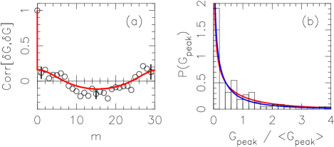
FIG. 3.: Conductance statistics: (a) peak-to-peak correlation function and (b) probability distribution of $G$ for the stadium data in Fig. 1. The numerical correlation function (circles with typical error bars)– the average of all pairs of peaks $m$ peaks apart– is in good agreement with the semiclassical theory (red). The agreement for small $m$ is surprising since this regime is not semiclassical, but shows how dynamics can give rise to correlations even between nearest-neighbors. The numerical probability distribution (histogram) is for the entire range of data in Fig. 1 and is compared to both the semiclassical theory (red) and the standard statistical theory based on random wavefunctions (blue). The two theories predict nearly the same result for this quantity, and both are consistent with the numerics.

In Fig. 1 we show an example trace of $G$ for the stadium. The calculation clearly demonstrates both strong peak-to-peak fluctuations and an oscillatory modulation of the heights (3 periods are observed). While the former comes from the quasi-random fluctuations in the wavefunctions near the leads, the large oscillatory modulation is caused by interference along the horizontal orbit which connects both leads.

Since the main theoretical result concerns the periodic modulation of the peak heights, it is natural to consider the Fourier power spectrum of $G_{\rm peak}(k)$. In Fig. 2 we present a comparison of the numerical and semiclassical power spectra, calculated for both integrable (circular) and chaotic (stadium) dots. The data show that for both the circle and the stadium the power spectrum has sharp peaks corresponding to periodic orbits. More peaks appear for narrow leads [Fig. 2(a)] because the lack of momentum constraint in this regime allows coupling to more periodic orbits. The excellent agreement between the semiclassical expression and the numerical result in all cases is a striking demonstration of the validity of our theory.

Further characterization of the peak fluctuations is shown in Fig. 3. The peak-to-peak correlation function is

$${\rm Corr}_{m}\left[\delta G,\delta G\right]\equiv\frac{\langle\delta G\left(E_{n+m}\right)\delta G\left(E_{n}\right)\rangle_{n}}{\langle\delta G\left(E_{n}\right)^{2}\rangle_{n}},$$ (12)

where $\delta G\left(E_{m}\right)\equiv G\left(E_{m}\right)-\langle G\left(E_{n}\right)\rangle_{n}$ is a natural measure of the statistics of nearby peaks. A semiclassical expression for this quantity can be derived by assuming that the distribution of individual peak heights is locally Porter-Thomas[24], with the mean given by the semiclassical envelope (3). Indeed, as was first shown by Kaplan and Heller [15], this is generally true for wavefunction fluctuations in chaotic systems. We obtain

$${\rm Corr}_{m} = \delta_{m,0}+\left(1-\delta_{m,0}\right)\times\frac{\sum_{\mu}A_{\mu}^{2}\cos\left(\frac{\tau_{\mu}\Delta}{\hbar}m\right)}{4\bar{\Gamma}^{2}+3\sum_{\mu}A_{\mu}^{2}}\,.$$ (13)

In Fig. 3(a) we compare the semiclassical correlation function with numerical data for the stadium dot. The oscillatory behavior for large separations reflects the peak in the corresponding power spectrum in Fig. 2 and is in agreement with the semiclassical result. The positive correlation for nearest neighbors is also in agreement with the semiclassical theory, demonstrating the influence of dynamics even in this apparently non-semiclassical regime.

When $T\!\gg\!\Delta$, the major source of correlations between neighboring peaks is the joint contribution of several resonances to the same conductance peak[9]. In this regime the “nearest-neighbor” correlator is ${\rm Corr}_{m=1}\!\sim\!1$, and the dynamical effect accounts for only a small correction to the correlation function. However, for low temperature $T\!\leq\!\Delta$, the correlations due to temperature are exponentially suppressed. In this regime, the correlations induced by dynamical modulation dominate, and they account for the experimentally observed enhancement of correlations at low temperatures[8].

The probability distribution of $G_{\rm peak}$ over a large energy range is the main quantity considered in the previous statistical theories[2, 3]. They predict no peak-to-peak correlation or periodic modulation of the heights, and a Porter-Thomas distribution: $P(G_{\rm peak})=\sqrt{4/\pi G_{\rm peak}}\exp(-G_{\rm peak})$. Considering an energy range larger than any period in Eq. (3), we find, in contrast, that the distribution should be locally Porter-Thomas but with the mean modulated by the periodic components, as in Ref. [15]. Curiously, the resulting distribution is not very different from Porter-Thomas: Fig. 3(b) shows that the two theories predict nearly the same result, and both are consistent with numerical calculation. This explains why no dynamical effect was observed in the experimental peak-height probability distribution[5, 6].

In contrast, the periodic modulation of the peak heights has been observed in several recent experiments[6, 7, 8]. The clearest observation is in Ref. [8]: the data in their Fig. 1 show modulated peak heights as a function of the number of electrons in the dot. In their trace of 90 peaks, approximately six oscillations are visible, yielding a period of $\sim\!15$ peaks. In our treatment, this period is the ratio of the period of fundamental oscillation in Eq. (3) to the level spacing $\Delta$. The fundamental period is given by $\left(\frac{1}{\hbar}\frac{\partial S_{\mu}}{\partial\varepsilon}\right)^{-1}\equiv\hbar/\tau_{\mu}$ where $\tau_{\mu}$ is the period of the relevant orbit. To determine $\tau_{\mu}$, we use the billiard approximation: $L_{\mu}\equiv v_{F}\tau_{\mu}$, where $L_{\mu}$ is the length of the shortest orbit and $v_{F}$ is the Fermi velocity. We use the micrograph of the dot to estimate $L_{\mu}$ for the $V$-shaped orbit connecting the two leads, and calculate $v_{F}$ from the experimental density[25]. Using the appropriate spin-resolved level spacing $\Delta\!\!=\!10$ $\mu$eV (which is half of the spin-full value from excitation measurements in Ref. [8]), we find $\hbar/\tau_{\mu}\Delta\!\approx\!12$. Because the billiard approximation underestimates the period in a soft wall potential, this is a lower bound for the modulation period, and therefore our theory is in good agreement with the experiment.

Similarly, we make estimates which are consistent with the other two experiments showing variation as a function of number of electrons[5, 6]. A similar approach to the peak modulation as a function of magnetic field is in agreement with the experimental results[6, 7] as well. This agreement with experiment is perhaps surprising, since the adding of electrons changes the effective potential defining the dot; however, experiments on ”magnetofingerprints” of the peaks[26] suggest that this change is small while to affect the dynamical modulation one must substantially change the action of the shortest periodic orbit.

We close with two further experiments suggested by our results. First, if the tuning parameter used to change the number of electrons, such as a gate voltage, does not change the action of the dominant periodic orbit, then no modulation connected to that orbit should be seen. In particular, gates which affect different parts of the dot may produce different oscillatory behavior. Second, several samples made in a robust geometry– a circle with directly opposite leads, for example– should show the same modulation. Any deviations from the same behavior would be a sensitive indication of the material quality.

We gratefully acknowledge stadium eigenfunction calculations by J. H. Lefebvre, helpful discussions with C. M. Marcus, the hospitality of the Aspen Center for Physics where this work was initiated, and support from the US ONR and the US NSF.

- [1] H. Grabert and M. H. Devoret, Single Charge Tunneling: Coulomb Blockade Phenomena in Nanostructures (Plenum Press, New York, 1992).
- [2] R. A. Jalabert, A. D. Stone, and Y. Alhassid, Phys. Rev. Lett. 68, 3468 (1992).
- [3] L. P. Kouwenhoven, C. M. Marcus, P. L. McEuen, S. Tarucha, R. M. Westervelt, and N. S. Wingreen, in Mesoscopic Electron Transport, edited by L. L. Sohn, L. P. Kouwenhoven, and G. Schön (Kluwer, Dordrecht, 1997) pp. 105-214.
- [4] M. Stopa, Physica B 251, 228 (1998).
- [5] A. M. Chang, H. U. Baranger, L. N. Pfeiffer, K. W. West, and T. Y. Chang, Phys. Rev. Lett. 76, 1695 (1996).
- [6] J. A. Folk, S. R. Patel, S. F. Godijn, A. G. Huibers, S. M. Cronenwett, and C. M. Marcus, Phys. Rev. Lett. 76, 1699 (1996).
- [7] S. M. Cronenwett, S. R. Patel, C. M. Marcus, K. Campman, and A. G. Gossard, Phys. Rev. Lett. 79, 2312 (1997).
- [8] S. R. Patel, D. R. Stewart, C. M. Marcus, M. Gök cedag, Y. Alhassid, A. D. Stone, C. I. Duruöz, and J. S. Harris, Jr., Phys. Rev Lett. 81, 5900 (1998).
- [9] Y. Alhassid, M. Gokcedag, and A. D. Stone, Phys. Rev. B 58, 7524 (1998).
- [10] M. Stopa, Phys. Rev. B 54, 13767 (1996).
- [11] G. Hackenbroich, W. D. Heiss, and H. A. Weidenmüller, Phys. Rev. Lett. 79, 127 (1997).
- [12] M. Gutzwiller, Chaos in Classical and Quantum Mechanics (Springer, New York, 1990).
- [13] J. B. Delos and C. D. Schwieters, in Classical, Semiclassical and Quantum Dynamics in Atoms, Lecture notes in physics 485, ed. by H. Friedrich and B. Eckhardt, p. 223-247, Springer (1997); M. W. Beims, V. Kondratovich, and J. B. Delos, Phys. Rev. Lett. 81, 4537 (1998).
- [14] E. J. Heller, in Chaos and Quantum Physics, edited by M. J. Giannoni, A. Voros, and J. Zinn-Justin (Elsevier, Amsterdam, 1991) pp. 547-663.
- [15] L. Kaplan, Phys. Rev. Lett 80, 2582 (1998); L. Kaplan, and E. J. Heller, Annals of Phys. 264, 171 (1998).
- [16] D. Weiss, K. Richter, A. Menschig, R. Bergmann, H. Schweizer, K. von Klitzing and G. Weimann, Phys. Rev. Lett. 70, 4118 (1993); G. Hackenbroich, and F. von Oppen, Europhys. Lett., 29, 151 (1995); K. Richter, Europhys. Lett. 29, 7 (1995).
- [17] E. E. Narimanov, A. D. Stone, and G. S. Boebinger, Phys. Rev. Lett. 80, 4024 (1998); an alternative semiclassical theory of resonant magnetotunneling was developed by E. B. Bogomolny, and D. C. Rouben, Europhys. Lett. 43, 111 (1998).
- [18] T. S. Monteiro, D. Delande, A. J. Fisher, G. S. Boebinger, Phys. Rev. B 56, 3913 (1996).
- [19] E. E. Narimanov, and A. D. Stone, to be published in Physica D; also preprint cond-mat/9808161.
- [20] C. W. J. Beenakker, Phys. Rev. B 44, 1646 (1991).
- [21] J. Bardeen, Phys. Rev. Lett. 6, 57 (1961).
- [22] The expressions given for and are for tunneling from a single subband in the lead. The generalization to many subbands is straightforward.
- [23] T. Szeredi, J. H. Lefebvre, D. A. Goodings, Nonlinearity 7, 1463 (1994).
- [24] L. E. Reichl, The Transition To Chaos (Springer-Verlag, New York, 1992).
- [25] C. M. Marcus, private communication.
- [26] D. R. Stewart, D. Sprinzak, C. M. Marcus, C. I. Duruöz, and J. S. Harris, Science 278, 1784 (1997).