Steady-State Cracks in Viscoelastic Lattice Models

Abstract

We study the steady-state motion of mode III cracks propagating on a lattice exhibiting viscoelastic dynamics. The introduction of a Kelvin viscosity $\eta$ allows for a direct comparison between lattice results and continuum treatments. Utilizing both numerical and analytical (Wiener-Hopf) techniques, we explore this comparison as a function of the driving displacement $\Delta$ and the number of transverse sites $N$. At any $N$, the continuum theory misses the lattice-trapping phenomenon; this is well-known, but the introduction of $\eta$ introduces some new twists. More importantly, for large $N$ even at large $\Delta$, the standard two-dimensional elastodynamics approach completely misses the $\eta$-dependent velocity selection, as this selection disappears completely in the leading order naive continuum limit of the lattice problem.

I Introduction

Recently, there has been renewed interest in the subject of dynamic fracture [2]. This has been sparked in large part by a set of experiments [3, 4] that have called into question some of the predictions of the traditional, continuum mechanics approach to fracture propagation. Specifically, it has been shown that cracks exhibit a branching instability long before they reach the predicted limiting speed of advance; this instability leads to enhanced dissipation and effectively prevents much additional acceleration. Although there are some hints of this instability in the continuum approach [5], attempts at a systematic analysis [6] have been inconclusive.

In this work, we adopt the philosophy of Marder and Gross [7] and consider lattice models of fracture. These models provide an invaluable test-bed for deciding when and if a continuum formulation is appropriate. After all, if the tip of a brittle crack really occurs at the scale of the lattice, there is no a priori reason for suspecting that a continuum approach could get the correct behavior. It is already clear, for example, that lattice models exhibit a sharp (sometimes discontinuous) jump from static cracks to propagating ones; this is not reproducible if one neglects lattice scale effects. One might hope, though, that at larger velocity there is some effective continuum description, perhaps utilizing the cohesive zone approach of Barenblatt [8]. From our perspective, it is an open issue as to whether any such model can accurately predict the behavior of some specific microscopic dynamical system exhibiting fracture.

Historically, lattice models of fracture received a major impetus from the work of Slepyan [9], who used the Wiener-Hopf technique to solve for steady-state propagation. In his work, he considered the case of infinitesimal dissipation. This fact made it difficult to carry out explicit comparisons between lattice results and continuum predictions thereof, inasmuch as the latter allows steady-state motion only at the limiting wave speed. One needs dissipative terms so as to introduce a new macroscopic velocity scale in order to allow more general steady-state continuum solutions. Subsequent analyses by Marder and collaborators [7, 10] did introduce dissipation in the form of a Stokes term; however, they did not explicitly consider the lattice-continuum comparison. In this paper, we introduce dissipation in a different form by adding a Kelvin viscosity term to the equation of motion. We will see that the advantage of this choice is that the continuum model is in fact an accurate approximation to the lattice dynamics at large enough $\eta v$. Note too that from a physics perspective, this type of viscoelasticity appears to have a marked effect on the crack stability [11] and is therefore interesting in its own right.

In this paper, we choose the simplest nonlinear form for the lattice springs, namely that the spring becomes completely broken (with no residual force) once it is stretched beyond some threshold. In a future publication, we will extend our analysis and results to a more general nonlinear force law. This generalization appears to change very little qualitatively with respect to the steady-state problem, although it is crucial in allowing for a direct calculation of the linear stability of the propagating fracture. As mentioned above, this stability issue is perhaps the one of most immediate relevance as far as the connection to experiments is concerned. But, as we shall see, the steady-state problem we solve here offers quite a few subtle and interesting aspects.

The organization of the paper is as follows. First, we introduce the lattice model, and discuss its basic energetic thresholds. We also briefly discuss the static arrested crack solutions. In the next section, we generalize the procedure we employed for finding the static solutions to solve for steady-state moving cracks for the case of one row of mass points ($N=1$), employing as a foundation the Slepyan ansatz for the form of the discrete steady-state solution. We analyze the dependence of the velocity on the driving displacement, studying the effect of the various parameters. The most important of these parameters is the viscosity. In the following section, we compare these results to a naive continuum limit, finding that whereas this naive continuum limit successfully reproduces the large-velocity regime, it fails to account for the nonexistence of solutions below a driving threshold. We then extend our method to arbitrary $N$, again solving for the dependence of the crack velocity on the driving displacement, as a function of the other parameters. Subsequently, we again compare our results to those of our naive continuum limit. In particular, we focus on the large $N$ limit, demonstrating how in this limit the standard continuum calculation is recovered. We find the surprising result that whereas the large-scale structure of the displacement field is almost completely insensitive to the crack velocity for velocities less than the wave-speed, the small-scale structure is extremely sensitive. Thus the whole velocity selection is completely a function of the lattice-scale dynamics, which no continuum theory can reproduce correctly. We conclude with directions for the future and some general observations.

II Model, Energetics and Statics

We study in this paper the Slepyan lattice model [9] for Mode III fracture, generalized to include Kelvin viscosity. The model consists of N infinitely long rows of mass points (with unit mass) coupled horizontally and vertically by damped “springs”. The bottom and top rows are anchored by “springs” to lines. The system is loaded by extending the top row a distance $\Delta$. The springs all have spring constant $1$, except for the bottom row, which has spring constant $k$. All the springs have a viscous damping $\eta$. The bottom springs break when their extension exceeds some threshold $\epsilon$. We label the (scalar) displacement of the $(i,j)$ mass from its unstressed equilibrium position as $u_{i,j}$. The equation of motion for $u_{i,j}$ reads

$${\ddot{u}}_{i,j}=(1+\eta\frac{d}{dt})(u_{i+1,j}+u_{i-1,j}+u_{i,j+1}+u_{i,j-1}-4u_{i,j})$$ (1)

for $j\neq 1$ with $u_{i,N+1}\equiv\Delta$, and

$${\ddot{u}}_{i,1}=(1+\eta\frac{d}{dt})(u_{i+1,j}+u_{i-1,j}+u_{i,2}-3u_{i,j})-k\theta(\epsilon-u_{i,1})(1+\eta\frac{d}{dt})u_{i,1}\ .$$ (2)

Of particular interest is the case $k=2$, which is equivalent to the problem of an up-down symmetric crack, joined at the fracture line by springs of strength $1$.

There are a number of important strain thresholds which can be understood from energetics and statics. The first is the point at which the uniformly stressed state cracks catastrophically. For our model in which the bottom spring has spring constant $k$ and the other vertical springs has spring constant $1$, for a (horizontally) uniform state, the equilibrium displacements are given by

$$u_{i,j}=u_{j}^{U}=\frac{(j-1)k+1}{Nk+1}\Delta\,$$ (3)

so that the strain of each spring is $k\Delta/(1+Nk)$, except for the bottom ’$k$’ spring which has strain $\Delta/(1+Nk)$. The system will fail catastrophically if the strain of the $k$ spring exceeds $\epsilon$ and this gives us our first threshold,

$$\Delta_{U}=\epsilon(Nk+1)$$ (4)

The second strain threshold is the Griffith’s criterion, which is the $\Delta$ at which the uniformly strained state becomes metastable with respect to the cracked state. The energy per column of the cracked state, $u_{i,j}=\Delta$, is just the energy to stretch the $k$ spring to cracking, $\frac{1}{2}\epsilon^{2}$, whereas the energy of the uniformly stressed state is

$${\cal E}_{U}=\frac{k\Delta^{2}}{2(Nk+1)}\ .$$ (5)

The cracked state is thus energetically favored when $\Delta$ exceeds

$$\Delta_{G}=\epsilon\sqrt{Nk+1}$$ (6)

Note that this is much smaller than $\Delta_{U}$ for large $N$.

This system is known to possess stationary solutions which represent semi-infinite arrested cracks. For completeness, and to begin to build the machinery we will need to treat the moving crack, we briefly outline the solution for this arrested crack. We choose $x=0$ to be the position of the last uncracked spring. We solve separately the problem in the uncracked $(x>0)$ and cracked $(x<0)$ regions and then tie the answers together. To solve, we need to know the normal modes of the vertical springs in the two regions. We define the general $N\times N$ coupling matrix as

$${\cal M}_{N}(m)=\left[\begin{array}[]{ccccccc}-(m+1)&1&&&&&\\ 1&-2&1&&&&\\ &1&-2&1&&&\\ &&&\ddots&&&\\ &&&&1&-2&1\\ &&&&&1&-2\end{array}\right]$$ (7)

The coupling matrix on the uncracked side is ${\cal M}_{N}(k)$ while on the cracked side it is ${\cal M}_{N}(0)$. Denote the eigenvectors of ${\cal M}_{N}(0),\ {\cal M}_{N}(k)$ as $\xi_{n},\Xi_{n}$, with eigenvalue $\lambda_{n},\Lambda_{n}$, $i=1,\ldots,N$. (Here and in the following lower (upper) case symbols refer to quantities on the cracked (uncracked) side).

The equation of equilibrium on either side reads

$$0=u_{i+1,j}-2u_{i,j}+u_{i-1,j}+{\cal M}_{N;j,j^{\prime}}(m)u_{i,j^{\prime}}$$ (8)

The general decaying solution on the uncracked side, $i\geq 0$, is

$$u_{i,j}=u^{U}_{j}+\sum_{n}^{N}A_{n}(\Gamma_{n})^{i}(\Xi_{n})_{j}$$ (9)

where $u^{U}$ is the uniformly strained solution presented above and

$$\Gamma_{n}=1-\frac{1}{2}\Lambda_{n}-\sqrt{-\Lambda_{n}+\frac{1}{4}(\Lambda_{n})^{2}}$$ (10)

governs the spatial decay of the $n$th mode, and satisfies $(\Gamma_{i})^{2}-(2-\Lambda_{i})\Gamma_{i}+1=0$.

The solution on the cracked side, $i\leq 0$, is similar:

$$u_{i,j}=\Delta-\sum_{n}^{N}a_{n}(\gamma_{n})^{i}(\xi_{n})_{j}$$ (11)

where

$$\gamma_{n}=1-\frac{1}{2}\lambda_{n}+\sqrt{-\lambda_{n}+\frac{1}{4}(\lambda_{n})^{2}}$$ (12)

This solution has $2N$ unknowns, $\{A_{n},a_{n}\}$. The equality of the two different expressions for $u_{0,j}$ provides $N$ equations. The equation of motion for $x=0$ provides the other $N$ equations. Solving this $2N\times 2N$ inhomogeneous system yields the desired answer. The range of validity of this solution is determined by the conditions that $u_{0,1}<\epsilon<u_{-1,1}$, so that the spring at $i=0$ is the last unbroken spring.

Doing this, we find that the possible $\Delta$’s span a range, $\Delta_{A}^{-}<\Delta<\Delta_{A}^{+}$ that encompasses the Griffith’s value $\Delta_{G}$. Above $\Delta_{A}^{+}$ the crack has to run, for it has no other alternative. Below $\Delta_{A}^{-}$, any initial crack would head itself.

In Fig. 1, we look at $\Delta_{A}^{\pm}/\Delta_{G}$ as a function of width for the natural case, $k=2$, and the case $k=.2$, where the material has been weakened along the incipient crack surface. As can be seen, the effect of the width, $N$, is to widen the window, but the effect is quite small, once things are normalized to $\Delta_{G}$. The convergence is numerically consistent with a $O(1/N)$ behavior. We see that $k$, on the other hand, has a dramatic effect, closing the size of the allowed window significantly.

III Moving Cracks, $N=1$

We now look at moving cracks, starting for simplicity with the case $N=1$. The key is the Slepyan traveling wave ansatz

$$u_{i}(t)=u(t-x/v)$$ (13)

We thus only need to find the function of one variable $u(t)$. Plugging this ansatz into the equation of motion, we get a differential-difference equation which is non-local in time:

$$\ddot{u}(t)=(1+\eta\frac{d}{dt})[u(t+1/v)-3u(t)+u(t-1/v)]-k\theta(\epsilon-u(t))(1+\frac{d}{dt})u(t)+\Delta$$ (14)

We choose $t=0$ to be the moment at which $u$ exceeds $\epsilon$, so we can replace the step function above by $\theta(-t)$. As in the static case, we solve the equation separately in the cracked ($t>0$) and uncracked ($t<0$) regions. It is convenient to discretize time with a small time-step $dt$, so that $t_{i}=i\,dt$. Then the solution for the uncracked side is

$$u(t_{i})=u^{U}+\sum_{l}A_{l}(\Gamma_{l})^{i}$$ (15)

where now the $\Gamma$ are given by those roots of

$$\frac{1}{dt^{2}}(\Gamma-2+\frac{1}{\Gamma})-\left[1+\frac{\eta}{dt}(1-\frac{1}{\Gamma})\right]\left[\Gamma^{n_{b}}-3-k+\Gamma^{-n_{b}}\right]\ .$$ (16)

which lie outside the unit circle. The number $n_{b}=1/(vdt)$ is constrained to be an integer, which implies that our resolution in $v$ is limited by our resolution in $dt$. There are $2n_{b}+1$ roots of this polynomial, (for $\eta\neq 0$), some number, $n_{u}$, of which lie outside the unit circle and thus give rise to a $u$ which converges as $t\to-\infty$. Thus, the solution for negative $t$ is parameterized by $n_{u}$ coefficients $A_{l}$, $l=\{1,2,\ldots,n_{u}\}$. Similarly, we solve in the cracked region, and the solution is now parameterized by $n_{c}$ coefficients $a_{l}$ corresponding to the roots of Eq. (16) (with $k$ set to zero) which lie inside the unit circle. It can also be shown that for sufficiently small $dt$, $n_{u}+n_{c}=2n_{b}+1$. Thus the entire solution is parameterized by $2n_{b}+1$ parameters. As in the static case, the two solutions overlap, this time for $2n_{b}$ values of $t_{i}$, $i=-n_{b},-n_{b}+1,\ldots,n_{b}-1$, so the last uncracked equation at $i=-1$ fixes $u$ out to $i=n_{b}-1$ and the last cracked equation at $i=1$ likewise fixes $u$ down to $i=-n_{b}$. The identity of the two expressions for $u$ in the overlap region give us $2n_{b}$ equations. The last equation we need comes from the equation of motion at the crack point $i=0$. Solving this inhomogeneous system gives us our desired solution. Reading off $u_{1}(0)=\epsilon$ gives us the relation between $v$ and $\Delta/\epsilon$ we need.

FIG. 1.: $\Delta_{A}^{\pm}/\Delta_{G}$ vs. N for the case $k=2,0.2$

Again, as in the static problem, there is a consistency constraint on the solution, namely that $u_{1}(t)$ not reach $\epsilon$ before $t=0$. In the $\eta=0$ problem studied by Marder, this happens for too small $v$. This holds true, as we shall see, for sufficiently small $\eta$.

In Fig. 2, we present data on $v$ versus $\Delta/\Delta_{G}$ for two values of $\eta=0.2,\ 2$ with $k=2$. Two striking features present themselves. First is the divergence of the velocity, which occurs for both values of $\eta$ at $\Delta_{U}$ which we calculated in Sec. 2 as the displacement for which the entire system wants to break apart. Note that in this model, there is nothing wrong with $v>1$, the wave speed in our units. The second important feature of these curves is the different behaviors exhibited at the left edge of the graph. The low $\eta$ graph exhibits the typical behavior of a subcritical bifurcation which ends at a square-root type cusp. The continuation past the cusp to even lower velocities is a numerical artifact of finite $dt$ and vanishes in the $dt\to 0$ limit. This cusp feature persists in the $\eta\to 0$ limit, and for smaller velocities the solutions are inconsistent with the condition mentioned above that $u(i)<\epsilon$ for $t<0$ and so are unphysical. For larger $\eta$, where the system is sufficiently overdamped, the solutions persist to zero velocity. However, the dependence on $\Delta/\Delta_{G}$ is very singular, and the graph approaches zero velocity at $\Delta_{A}^{+}$ exponentially in $1/v$. Before proceeding to a full survey of parameter space, it is useful to develop a naive continuum limit for our system, which is analytically more tractable and serves as a useful benchmark for our discussions. We do this in the next section.

FIG. 2.: $v$ versus $\Delta/\Delta_{G}$ for $\eta=0.2,\ 2$ for $N=1$, $k=2$. The calculation was done with $dt=.05$. The solid lines are the naive continuum results for the same parameters.

IV Naive Continuum Limit

We now develop the naive continuum limit of the equation of motion for $N=1$ steady-state moving cracks. We obtain this limit by simply replacing the finite difference by a derivative, yielding:

$$\ddot{u}(t)=(1+\eta\frac{d}{dt})\left(\frac{1}{v^{2}}\frac{d^{2}u}{dt^{2}}-u\right)-k\theta(-t)(1+\eta\frac{d}{dt})u+\Delta$$ (17)

The solution for $t<0$ is

$$u(t)=\frac{\Delta}{1+k}+A_{1}e^{Q_{1}vt}$$ (18)

where $Q_{1}$ is the unique root with positive real part of the polynomial $P(-(1+k);Q_{1})$ where in general $P(\lambda;Q)$ is defined by

$$P(\lambda;Q)\equiv\eta vQ^{3}+(1-v^{2})Q^{2}+(1+\eta vQ)\lambda\;.$$ (19)

In general, for $\lambda<0$, $P$ has one positive root, with the other roots having negative real parts. Similarly, the solution for $t>0$ is

$$u(t)=\Delta-a_{2}e^{-q_{2}vt}-a_{3}e^{-q_{3}vt}$$ (20)

where $-q_{2}$, $-q_{3}$ are the two roots with negative real part of $P(-1;q)$ One can solve for $A_{1}$, $a_{2}$, and $a_{3}$ by using the continuity of $u$ and its first two derivatives at $t=0$.

One can learn a few things from these equations. As pointed out by Langer in his study of a related model [12], vanishing $\eta$ in the continuum is a singular limit, since it controls the highest derivative. Secondly, the special role of the wave speed, $v=1$, is clear. Most interesting, however, is the question of when we expect this continuum limit to be valid. The condition is that at least some of the exponential decay rates are small, such that the solution will look smooth on the lattice scale. For small $v$, $Q_{1}\sim\sqrt{k+1}$, $q_{2}\sim 1$, and $q_{3}\sim 1/(\eta v)$, so none of the $q$’s are small and the continuum limit is not reliable. For large $v$, things are different. Here, $Q_{1}\sim v/\eta$, $q_{2,3}\sim(\eta\pm\sqrt{\eta^{2}-4})/(2v)$. The large value of $Q_{1}$ corresponds to the existence of a boundary layer which allows for the matching of the highest derivative term. If this boundary layer does not affect the lower order matches (as is fairly typical), then we would expect that the continuum result will agree with the lattice answer.

It is straightforward to work out the small velocity limit of the continuum theory. Using the limiting values of the $q$’s above, and solving the linear system, one gets that $\epsilon\sim\Delta/\sqrt{k+1}+O(v)$, so that $\Delta\sim\Delta_{G}+O(v)$. Thus, the continuum solution starts at the Griffith’s point $\Delta_{G}$ with zero velocity and the velocity grows linearly as $\Delta$ is increased. Continuing the calculation to first order in $v$, we find $v=(\Delta/\Delta_{G}-1)/[(\sqrt{k+1}-1)\eta]$. Thus, the velocity is inversely proportional to $\eta$. This is as expected, since for $v\ll 1$, the velocity only enters in the combination $\eta v$.

The large velocity limit is also analyzable. Again using the $q$’s found above, we obtain to leading order that $v=\left[(1-\Delta_{U})/(k\eta^{2})\right]^{-1/4}$ so that $v$ diverges at $\Delta_{U}$. Note also that in this regime $v$ scales as $\sqrt{\eta}$, so that as viscosity increases so does the velocity. This is because the only reason that propagation at $v>1$ is possible is because of the viscosity, so the larger the viscosity the more efficient the propagation.

As $\eta$ goes to zero, the continuum limit must break down. The velocity increases very rapidly (at a rate proportional to $1/\eta$) to near $1$, and stays there till $\Delta$ is near $\Delta_{U}$, whence it rapidly diverges. The velocity crosses unity at $\Delta=(1+k)^{2/3}$ with slope of order $\eta^{2/3}$. Thus, with vanishingly small $\eta$, steady-state propagation, at least in our naive continuum limit, is only possible at the wave speed $v=1$.

We are now in a position to compare our lattice calculation to the continuum results. For example, Fig. 2 above also displays the continuum curves. We see that in general the continuum calculation is very good only at the largest velocities. The agreement gets progressively worse for smaller velocities and breaks down completely for $\Delta$ less than the arrest value $\Delta_{U}^{+}$. This must be since the continuum calculation has the velocity going smoothly to zero at $\Delta_{G}$, which it never does due to the existence of arrested solutions. Also, the agreement is better at larger $\eta$; above some critical $\eta$, (about $\eta\approx 0.5$ for $k=2$), the continuum curve serves as an upper bound on the lattice curve and thus is a fair approximation until we start getting close to the arrest value. All of this is to be contrasted to what would have been obtained had we set $\eta=0$ and introduced instead a Stokes velocity term proportional to $\dot{u}$. Then, the continuum theory has a limiting velocity of $v=1$ and since this feature is not shared by the lattice dynamics, the continuum approximation would be nowhere accurate.

FIG. 3.: $\eta v$ versus $\Delta/\Delta_{G}$ for $\eta=1$, 1.5, 2, 4, 8 for $N=1$, $k=2$. The calculation was done with $dt=.05$.

We saw from the continuum calculation that for velocities $v\ll 1$, the relevant parameter for the continuum calculation is $\eta v$. We can test this for the lattice model by plotting $\eta v$ versus $\Delta$. This is presented in Fig. 3. We see that asymptotically for large $\eta$ this scaling sets in, but for finite $\eta$, the existence of the lattice length scale ruins the simple scaling.

It is interesting to see what happens for smaller $k$. We saw that the window of arrested solutions is significantly smaller for smaller $k$. In Fig. 4, we present the analog of Fig. 2, but this time with $k=0.2$. We see that the results are as far from the continuum limit as they were with the larger $k$. While the window of arrested solutions is smaller, so is the value of $\Delta_{U}/\Delta_{G}$, so the entire picture is just shrunk to a smaller range of $\Delta$.

A Wiener-Hopf Solution

Before we turn to general $N$, we will present the equivalent Wiener-Hopf solution of the $N=1$ problem. This method is more involved for the case $N=1$, but it is a model for the Wiener-Hopf solution we will present for general $N$, which we allow us to draw analytical conclusions in the large $N$ limit. The basic method follows that of Marder and Gross [7], but the presence of viscosity adds some new twists which are worthy of comment.

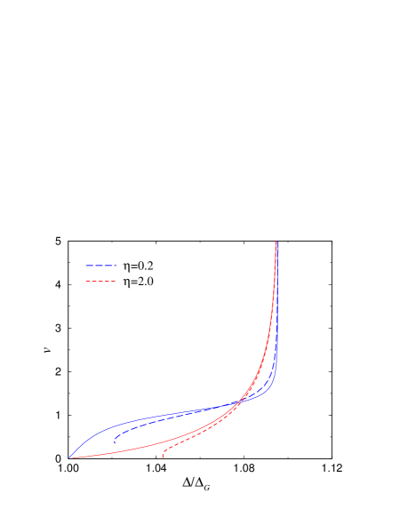
FIG. 4.: $v$ versus $\Delta/\Delta_{G}$ for $\eta=0.2,\ 2$ for $N=1$, $k=0.2$. The calculation was done with $dt=.05$. The solid lines are the naive continuum results for the same parameters.

To begin, we define the Fourier-transform ${\tilde{u}}^{\pm}$ of the right- and left-hand pieces of the $u$ field as follows:

$${\tilde{u}}^{\pm}(K)=\int_{-\infty}^{\infty}\,vdt\ \theta(\pm t)e^{iKvt}u(t)$$ (21)

It should be noted that ${\tilde{u}}^{\pm}$ are analytic in the upper and lower half-planes respectively. The Fourier transform of the $u$ field, $\tilde{u}$, is just the sum of the two parts: $\tilde{u}(K)={\tilde{u}}^{+}+{\tilde{u}}^{-}$. In terms of these fields, the equation of motion reads

$$0=\left(i\eta vK^{3}-(1-v^{2})K^{2}\right){\tilde{u}}-(1-i\eta vK){\tilde{u}}-k(1-i\eta vK){\tilde{u}}^{-}+\Delta\delta(K)-k\eta vu(0)$$ (22)

The last term is noteworthy, and arises because the time derivative does not act on the $\theta$-function in the last term in Eq. 17. Expressing $\tilde{u}$ in terms of its component pieces, we recognize that the coefficients of ${\tilde{u}}^{\pm}$ are nothing put $P(-1;-iK)$, $P(-(1+k);-iK)$ respectively, that we encountered in our solution above, so that the the equation of motion reads

$$0=P(-(1+k);-iK){\tilde{u}}^{-}+P(-1;-iK){\tilde{u}}^{+}+\Delta\delta(K)-k\eta vu(0)$$ (23)

Next, we factor the $P$’s in terms of their roots

$$P(-(1+k);-iK) = i\eta v(K-iQ_{1})(K+iQ_{2})(K+iQ_{3})$$ (24)

$$P(-1;-iK) = i\eta v(K-iq_{1})(K+iq_{2})(K+iq_{3})$$ (25)

Dividing through by $i\eta v(K-iq_{1})(K+iQ_{2})(K+iQ_{3})$ we obtain

$$0=\frac{K-iQ_{1}}{K-iq_{1}}{\tilde{u}}^{-}+\frac{(K+iq_{2})(K+iq_{3})}{(K+iQ_{2})(K+iQ_{3})}{\tilde{u}}^{+}-\frac{\Delta}{\eta vq_{1}Q_{2}Q_{3}}\delta(K)+\frac{ik}{(K-iq_{1})(K+iQ_{2})(K+iQ_{3})}u(0)$$ (26)

where we have used the $\delta(K)$ to simplify its prefactor. We use the fact that $q_{1}q_{2}q_{3}=-P(-1;0)/(\eta v)=1/\eta v$ to rewrite our equation as

$$0=\frac{K-iQ_{1}}{K-iq_{1}}{\tilde{u}}^{-}+\frac{(K+iq_{2})(K+iq_{3})}{(K+iQ_{2})(K+iQ_{3})}{\tilde{u}}^{+}-\frac{\Delta q_{2}q_{3}}{Q_{2}Q_{3}}\delta(K)+\frac{ik}{(K-iq_{1})(K+iQ_{2})(K+iQ_{3})}u(0)$$ (27)

To proceed, we have to decompose the two inhomogeneous terms into pieces analytic in either the upper- or lower- half-planes. The result is

$$0 = \frac{K-iQ_{1}}{K-iq_{1}}{\tilde{u}}^{-}+\frac{(K+iq_{2})(K+iq_{3})}{(K+iQ_{2})(K+iQ_{3})}{\tilde{u}}^{+}-\frac{\Delta q_{2}q_{3}}{Q_{2}Q_{3}}\left(\frac{i}{K+i0^{+}}-\frac{i}{K-i0^{+}}\right)$$ (28)

$$\ +\frac{ik}{(q_{1}+Q_{2})(q_{1}+Q_{3})}\left(-\frac{1}{(K-iq_{1})}+\frac{K+i(q_{1}+Q_{2}+Q_{3})}{(K+iQ_{2})(K+iQ_{3})}\right)u(0)$$ (29)

The key to the Wiener-Hopf method is the realization that the sum of the terms analytic in either half-plane have to vanish, allowing us to solve for ${\tilde{u}}^{\pm}$. We find

$${\tilde{u}}^{+} = \frac{i\Delta q_{2}q_{3}(K+iQ_{2})(K+iQ_{3})}{Q_{2}Q_{3}(K+i0^{+})(K+iq_{2})(K+iq_{3})}-\frac{ik(K+i(q_{1}+Q_{2}+Q_{3}))}{(q_{1}+Q_{2})(q_{1}+Q_{3})(K+iq_{2})(K+iq_{3})}u(0)$$ (30)

$${\tilde{u}}^{-} = \frac{-i\Delta Q_{1}(K-iq_{1})}{(1+k)q_{1}(K-i0^{+})(K-iQ_{1})}+\frac{ik}{(q_{1}+Q_{2})(q_{1}+Q_{3})(K-iQ_{1})}u(0)$$ (31)

Notice that the poles in ${\tilde{u}}^{\pm}$ give rise to exactly the same exponential terms in $u$ that we found previously. It can be explicitly verified that the two forms of the solution are equivalent. For our purposes, it is sufficient to examine what happens in the small $v$ limit. Then, as we have already noted $q_{3},Q_{3}\approx 1/(\eta v)$. The first, $\Delta$, term on the right-hand sides approaches a finite limit, with $O(v^{2})$ corrections, whereas the second $u(0)$ term vanishes linearly in $\eta v$. More explicitly, we find

$${\tilde{u}}^{+}\approx\frac{i\Delta q_{2}q_{3}(K+iQ_{2})}{Q_{2}Q_{3}(K+i0^{+})(K+iq_{2})}-\frac{ik\eta v}{(q_{1}+Q_{2})(K+iq_{2})}u(0)$$ (32)

Using $q_{1}=q_{2}=1$, $Q_{1}=Q_{2}=\sqrt{1+k}$, and $q_{3}=Q_{3}=1/\eta v$, and using the inverse Fourier transform to evaluate this in the limit $x\to 0^{+}$, we obtain

$$u(0)=\frac{\Delta}{\sqrt{1+k}}-\frac{k\eta v}{1+\sqrt{1+k}}u(0)$$ (33)

Recognizing $u(0)=\epsilon$ and $\sqrt{1+k}=\Delta_{G}/\epsilon$, after reorganizing we obtain

$$\eta v=\left(\frac{\Delta}{\Delta_{G}}-1\right)\frac{1+\sqrt{1+k}}{k}$$ (34)

which is easily seen to be equivalent to what we obtained from the direct method. As can be appreciated, the Wiener-Hopf method is much more involved than the direct method. Nevertheless, it will be the essential tool for analyzing the large-$N$ limit.

V General $N$

It is straightforward to extend the lattice calculations to arbitrary N. The basic method is the same: we solve the problem on the two sides of the crack tip position and patch the two solutions together. The solution on either side is again a sum over modes, which are a direct product of modes in the vertical direction, given by the eigenmodes of ${\cal M}_{N}(m=0,k)$, with the modes in the horizontal direction. Thus there are a total of $Nn_{u}$ and $Nn_{c}$ modes on the uncracked and cracked sides, respectively. The solutions on either side have to overlap for each value of the vertical component $j$, so there are an appropriate number of equations for the unknown coefficients of each mode. As for $N=1$, the condition $u(0,1)=\epsilon$ is used to determine the driving $\Delta$ corresponding to a given velocity.

We can also generalize our continuum calculation to finite $N$. As in the $N=1$ case, we replace finite differences in $t$ with derivatives, giving us $N$ coupled third-order differential equations. Again, we can solve these exactly on either side of the crack tip $t=0$, and match the functions and their first and second derivatives at this point. The functions are characterized by $N$ modes on the uncracked side, with decay rates $Q_{1,n}$, and $2N$ modes on the cracked side, with decay rates $q_{2,n}$, $q_{3,n}$. For each $n$, $Q_{1,n}$ is the positive root of of the polynomial $P({\Lambda_{n}})$ defined in Eq. (19) above. Let us denote the other roots of this polynomial, which we will need later, by $-Q_{2,n}$, $-Q_{3,n}$. Similarly, $-q_{2,n}$, $-q_{3,n}$ are the two negative (real part) roots of $P(\lambda_{n})$. with the third, positive, root being labeled by $q_{1,n}$. Implementing these procedures, we again calculate the crack velocity as a function of $\Delta/\Delta_{G}$. Again, we compare this data to that of our naive continuum (in $x$) calculation for the same value of $N$. We present in Fig. 5 the results for our overdamped case $\eta=2$, for $N=1,2,5,10,15$. Qualitatively, not much changes with $N$. The most important feature in that the middle section of the curves get progressively flatter as $N$ increases. This must be the case, since the point of divergence, $\Delta_{U}$, measured in terms of $\Delta_{G}$, increases as $N^{1/2}$. We also note that the data for low velocities seems to converge fairly rapidly as $N$ increases, and the rate of convergence slows as $v$ increases. Again, as in the $N=1$ case, the continuum results accurately reproduce the lattice calculations for large $v$ and are completely wrong for small $v$, missing the lattice-induced arrest phenomenon.

FIG. 5.: $v$ versus $\Delta/\Delta_{G}$ for $\eta=2$ for $N=1,\ 2,\ 5,\ 10,\ 15$; $k=2$. The calculation was done with $dt=.1$. The solid lines are the naive continuum results for the same parameters.

VI Large N

The physical problem of cracking a macroscopic object corresponds to the limit of large, but finite, $N$. The lattice calculations are prohibitively expensive for too large $N$. However, our naive continuum calculations can be carried out for fairly large $N$’s. Using the fact that for small $v$, the convergence in $N$ is rapid, and for larger $v$, the naive continuum results are reliable, we can piece together a fairly complete picture of what we expect in the macroscopic limit. In particular, it is interesting to compare this with the standard continuum theory in order to understand the limitations and successes of that theory.

FIG. 6.: $v$ versus $\Delta/\Delta_{G}$ in the continuum approximation for for $N=10,\ 50,\ 200,\ 400$, with $\eta=2$, $k=2$.

To begin, we present in Fig. 6 the results of our naive continuum theory, extended to larger values of $N$. The most striking feature of this graph is the slow convergence that sets in near $v=1$. Exploring numerically, we find that for fixed $v<1$, the data converges with large $N$ as $N^{-1/2}$. However, the coefficient of this $N^{-1/2}$ correction becomes ever larger as $v$ approaches unity. Looking at the value of $\Delta/\Delta_{G}$ where $v=1$, it appears to be diverging as $N^{1/6}$ as $N\to\infty$. Thus, in the macroscopic limit, the crack speed is effectively bounded by the wave speed.

To proceed further in studying our naive continuum theory at large $N$, it is useful to derive the Weiner-Hopf solution. To do this, we first Fourier transform the fields, writing

$$u_{j}(t)=\int_{-\infty}^{\infty}\frac{dk}{2\pi}e^{-ivKt}{\tilde{u}}_{j}(K)$$ (35)

The equations for all $j\neq 1$ are translationally invariant in $t$, and become algebraic. The structure of these equations is

$$0=\left(i\eta vK^{3}-(1-v^{2})K^{2}\right){\tilde{u}}_{j}+(1-i\eta Kv){\cal M}_{N-1;j,j^{\prime}}(1){\tilde{u}}_{j^{\prime}}+\delta_{j,2}(1-i\eta vK){\tilde{u}}_{1}+\delta_{j,N}\Delta\delta(K)$$ (36)

Defining $f(K)\equiv(i\eta vK^{3}-(1-v^{2})K^{2})/(1-i\eta vK)$ and denoting the $n\times n$ identity matrix as ${\cal I}_{n}$, we can using Cramer’s rule explicitly solve for ${\tilde{u}}_{2}$ in terms of ${\tilde{u}}_{1}$ as follows

$${\tilde{u}}_{2}=-\frac{det_{N-2}\left(f(K){\cal I}+{\cal M}(1)\right)}{det_{N-1}\left(f(K){\cal I}+{\cal M}(1)\right)}{\tilde{u}}_{1}-\frac{(-1)^{N}\Delta}{det_{N-1}{\cal M}(1)}\delta(K)\;.$$ (37)

where in the last term we have used the $\delta(K)$ to simplify the determinant. To treat the $j=1$ with its step functions we define

$${\tilde{u}}^{\pm}=\int_{-\infty}^{\infty}\,vdt\ \theta(\pm t)e^{iKvt}u_{1}(t)$$ (38)

so that ${\tilde{u}}_{1}={\tilde{u}}^{+}+{\tilde{u}}^{-}$. The $j=1$ equation now reads

$$0=(1-i\eta vK)\left[(f(K)-1){\tilde{u}}_{1}-\frac{det_{N-2}\left(f(K){\cal I}+{\cal M}(1)\right)}{det_{N-1}\left(f(K){\cal I}+{\cal M}(1)\right)}{\tilde{u}}_{1}-k{\tilde{u}}^{-}\right]$$ (39)

$$\;\;\;\;\;\;\;-k\eta vu_{1}(0)-\frac{(-1)^{N}\Delta}{det_{N-1}{\cal M}(1)}\delta(K)$$ (40)

Multiplying through by $det_{N-1}\left({f(K){\cal I}+\cal M}(1)\right)/(1-i\eta vK)$, we get

$$0 = det_{N}(f(K){\cal I}+{\cal M}(0)){\tilde{u}}^{-}+det_{N}(f(K){\cal I}+{\cal M}(k)){\tilde{u}}^{+}$$ (41)

$$\ -\frac{k\eta vu_{1}(0)det_{N-1}(f(K){\cal I}+{\cal M}(1))}{1-i\eta vK}-(-1)^{N}\Delta\delta(K)$$ (42)

The determinants are easy to calculate in the diagonal bases of the $\cal M$’s, and have zeros at $K$’s corresponding precisely to $i$ times the roots of the polynomials $P(\Lambda_{n})$, $P(\lambda_{n})$ we encountered in our original real-space calculation. We can thus write

$$det_{N}(f(K){\cal I}+{\cal M}(k)) = \left(1-i\eta vK)\right)^{-N}\prod_{n=1}^{N}P(\Lambda_{n};-iK)$$ (43)

$$= \left(\frac{i\eta v}{1-i\eta vK}\right)^{N}\prod_{n=1}^{N}(K-iQ_{1,n})(K+iQ_{2,n})(K+iQ_{3,N})$$ (44)

and similarly

$$det_{N}(f(K){\cal I}+{\cal M}(0)) = (1-i\eta vK)^{-N}\prod_{n=1}^{N}P(\lambda_{n};-iK)$$ (45)

$$= \left(\frac{i\eta v}{1-i\eta vK}\right)^{N}\prod_{n=1}^{N}(K-iq_{1,n})(K+iq_{2,n})(K+iq_{3,N})$$ (46)

Similarly, if we denote the eigenvalues of ${\cal M}_{N-1}(1)$ by $\ell_{m}$, $m=1,\ldots,N-1$, we can express $det_{N-1}(f(K){\cal I}+{\cal M}(1))$ in terms of the roots $\chi_{1,m}$, $-\chi_{2,m}$, and $-\chi_{3,m}$ of $P(\ell_{m})$

$$det_{N-1}(f(K){\cal I}+{\cal M}(1)) = (1-i\eta vK)^{-N-1}\prod_{m=1}^{N-1}P(\ell_{m};-iK)$$ (47)

$$= \left(\frac{i\eta v}{1-i\eta vK}\right)^{N-1}\prod_{m=1}^{N-1}(K-i\chi_{1,m})(K+i\chi_{2,m})(K+i\chi_{3,m})\;.$$ (48)

We can then re-express Eq. 41 as

$$0 = \prod_{n}\frac{K-iQ_{1,n}}{K-iq_{1,n}}{\tilde{u}}^{-}+\prod_{n}\frac{(K+iq_{2,n})(K+iq_{3,n})}{(K+iQ_{2,n})(K+iQ_{3,n})}{\tilde{u}}^{+}$$ (49)

$$\;+\frac{ik\prod_{m}(K-i\chi_{1,m})(K+i\chi_{2,m})(K+i\chi_{3,m})}{\prod_{n}(K-iq_{1,n})(K+iQ_{2,n})(K+iQ_{3,n})}u_{1}(0)-\frac{\Delta}{(\eta v)^{N}\prod_{n}q_{1,n}Q_{2,n}Q_{3,n}}\delta(K)$$ (50)

$$= \prod_{n}\frac{K-iQ_{1,n}}{K-iq_{1,n}}{\tilde{u}}^{-}+\prod_{n}\frac{(K+iq_{2,n})(K+iq_{3,n})}{(K+iQ_{2,n})(K+iQ_{3,n})}{\tilde{u}}^{+}$$ (51)

$$\;+\frac{ik\prod_{m}(K-i\chi_{1,m})(K+i\chi_{2,m})(K+i\chi_{3,m})}{\prod_{n}(K-iq_{1,n})(K+iQ_{2,n})(K+iQ_{3,n})}u_{1}(0)-\Delta\prod_{n}\frac{q_{2,n}q_{3,n}}{Q_{2,n}Q_{3,n}}\delta(K)$$ (52)

where in the last step, we applied the identity

$$\prod_{n}q_{1,n}q_{2,n}q_{3,n}=(-\eta v)^{-N}det{\cal M}_{N}(0)=(\eta v)^{-N}\ .$$ (53)

and where we have used the easily verified fact that $det{\cal M}_{N}(m)=(-1)^{N}(mN+1)$. Note that this product result nicely reduces to the result we previously obtained for $N=1$. Again, as in the $N=1$ case, to proceed with the Wiener-Hopf method, we need to break up the last two terms into pieces analytic in the upper and lower half-planes. The $u_{1}(0)$ piece does not appear to have a simple breakup. However, for large $N$, the effect of this term becomes irrelevant, since $u_{1}(0)$ is a factor $N^{1/2}$ smaller than $\Delta$. The last term is easily broken up as we did in the $N=1$ case. We find that to leading order

$${\tilde{u}}^{+}\approx\Delta\left(\frac{i}{K+i0^{+}}\right)\prod_{n}\frac{q_{2,n}q_{3,n}(K+iQ_{2,n})(K+iQ_{3,n})}{Q_{2,n}Q_{3,n}(K+iq_{2,n})(K+iq_{3,n})}\ .$$ (54)

In the large $N$ limit, we can use this to evaluate $u$ explicitly. (We need not concern ourselves with ${\tilde{u}}^{-}$, since for $t<0$, $u_{1}(t)$ is always smaller that $u_{1}(0)$, and so does not contribute to leading order.) To proceed, we need the explicit form of the $q,Q$’s to leading order. As we shall see, the behavior is controlled by modes where $n<<N$. For these modes, we may approximate the eigenvalues of ${\cal M}_{N}(k)$ by $\Lambda_{1,n}=\Lambda_{2,n}=-n^{2}\pi^{2}/N^{2}$, so that $Q_{1,n}=Q_{2,n}=\frac{n\pi}{N\sqrt{1-v^{2}}}$, $Q_{3,n}=(1-v^{2})/(\eta v)$. (Here we have assumed that $v$ is less than and not too close to $1$.) Similarly, for ${\cal M}_{N}(0)$, we find $\lambda_{1,n}=\lambda_{2,n}=-(n-\frac{1}{2})^{2}\pi^{2}/N^{2}$, so that $q_{1,n}=q_{2,n}=\frac{(n-\frac{1}{2})\pi}{N\sqrt{1-v^{2}}}$, $q_{3,n}=(1-v^{2})/(\eta v)$. Notice that since $Q_{3,n}\approx q_{3,n}$, the factors involving these quantities cancel. This has the immediate consequence that the viscosity $\eta$ has completely dropped out of the problem in this limit.

The remaining expression has poles at $-i0^{+}$ and at $-iq_{2,n}$. We can evaluate the residue of each of these poles explicitly. The residue at $-i0^{+}$ is immediately seen to be

$$Res(e^{-iKvt}{\tilde{u}}^{+})|_{-i0^{+}}=i\Delta\ .$$ (55)

Evaluating the residues at the other poles is more complicated. To proceed, let us cut-off the product at some large $n\equiv N_{c}<<N$. Then, our approximate expressions for the $q$’s and $Q$’s are valid. This leads to

$$Res(e^{-iKvt}{\tilde{u}}^{+})|_{-iq_{2,n}} = -ie^{-\frac{(n-\frac{1}{2})\pi vt}{N\sqrt{1-v^{2}}}}\frac{\Gamma(N_{c}+\frac{1}{2})\Gamma(n-\frac{1}{2})\Gamma(N_{c}+\frac{3}{2}-n)}{(n-\frac{1}{2})\Gamma(N_{c}+1)\Gamma^{3}(\frac{1}{2})\Gamma(n)\Gamma(N_{c}+1-n)}$$ (56)

$$\simeq -ie^{-\frac{(n-\frac{1}{2})\pi vt}{N\sqrt{1-v^{2}}}}\frac{\Gamma(n-\frac{1}{2})}{(n-\frac{1}{2})\pi^{\frac{3}{2}}\Gamma(n)}\ +\ O(\frac{1}{N_{c}})$$ (57)

We then take the limit of $N_{c}\rightarrow\infty$ to find the final answer for the macroscopic displacement field

$$u_{1}(t) = \theta(t)\Delta\left[1\ -\ \sum_{n=1}^{\infty}\frac{\Gamma(n-\frac{1}{2})}{(n-\frac{1}{2})\pi^{\frac{3}{2}}\Gamma(n)}e^{-\frac{(n-\frac{1}{2})\pi vt}{N\sqrt{1-v^{2}}}}\right]$$ (58)

$$= \theta(t)\Delta\left(1-\frac{2}{\pi}\sin^{-1}{e^{-\frac{\frac{1}{2}\pi vt}{N\sqrt{1-v^{2}}}}}\right)$$ (59)

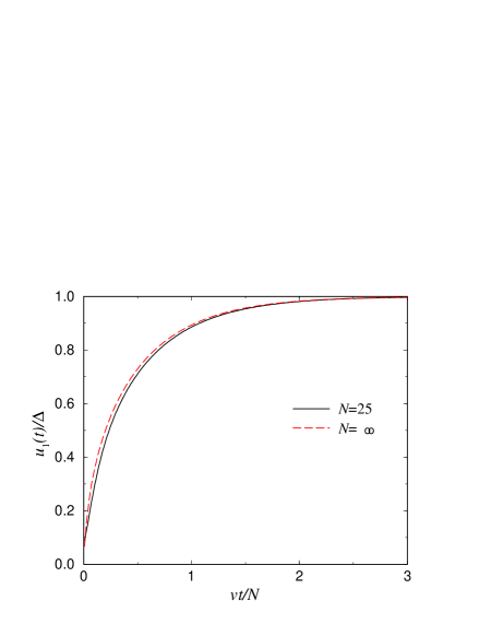
FIG. 7.: $u_{1}(t)/\Delta$ versus $vt/N$ in the continuum approximation for $k=2$, $\eta=2$, $N=25$, compared with the large-$N$ analytic result, Eq. (58).

This final answer exhibits the well-known square root branch cut at the crack tip location, $t=0$. It is worth noting that this behavior of the displacement gives rise to a macroscopic stress field which actually diverges as $\frac{1}{x^{3/2}}$ (recall the extra derivative due to the Kelvin viscosity) near the crack tip. This surprising finding renders invalid the 2-d continuum calculation of Langer[12] who studied this problem with the additional complication of a finite length cohesive zone. A correct continuum formulation which does reproduce the essential formula Eq. (54) is presented in the Appendix.

FIG. 8.: $u_{1}(t)/u_{\text{A}sympt}(t)$ versus $vt$ in the continuum approximation where $u_{\text{A}sympt}$ is the large-$N$ analytic result, Eq. (58), for $N=1,2,5,10,25$. Again, $k=2$, $\eta=2$.

A comparison of the above prediction with the numerically computed displacement is shown in Fig. (7) for the case $N=25$, plotted as a function of the macroscopic scale $vt/N$. We see that our large $N$ analytic result correctly reproduces the large-scale structure of the crack displacement. It does worse, though still quite accurate, close in to the crack tip. To demonstrate this more quantitatively, we present in Fig. (8) the ratio of the crack displacement $u_{1}(t)$ to the large-$N$ analytic result, for various $N$. Now the data is plotted as a function of the microscopic scale $vt$. We see that curves are all quite similar. They have a square-root divergence at the origin, since the analytic prediction is that $u(t)$ vanishes at $t=0$, whereas the true answer is finite. By $N=25$, they have converged to a limiting curve. This means that the finite-$N$ theory possesses a well-defined microscopic structure, in addition to the universal macroscopic structure defined by the standard continuum theory. This microscopic structure is on the scale of the lattice constant (in the $y$-direction) and is of course invisible to the standard continuum theory.

This observation implies that the entire issue of velocity selection via the condition that $u(x=0,y=1)$ be fixed to equal the breaking displacement is out of reach of the leading order macroscopic limit. Thus, as an example, the velocity depends explicitly on $\eta$ (as opposed to the macroscopic displacement which explicitly does not) even for arbitrarily large $N$. Conversely, calculating the macroscopic field in the continuum limit does not suffice for determining the crack speed which is always fixed at the lattice scale. Situations with equivalent macroscopic fields can have arbitrarily different crack velocities.

VII Summary

In this paper, we have studied in some detail the steady-state motion of mode III viscoelastic cracks in a lattice model of the microscopic dynamics. The most important finding are

1. The existence of a minimum velocity for crack propagation is dependent on the viscosity. At low $\eta$ (and indeed in the lattice models without dissipation that have been studied to date), the steady-state branch starts at finite $v$. For highly damped systems, on the other hand, the branch extends all the way to $v=0$ at the upper end of the allowed range of $\Delta$ for arrested cracks.

2. For finite $N$, a continuum approach (in $x$) for the crack does accurately predict the lattice results for values of the driving away from the lattice trapping (low or zero velocity) regime.

3. Taking the macroscopic limit ($N\rightarrow\infty$) allows us to recover the expected macroscopic behavior that the displacement grows as $\sqrt{x-x_{\mbox{tip}}}$ once we leave an inner core region of the lattice scale. The coefficient of this term can be calculated by using a continuum theory with the proper boundary conditions. A key feature of this macroscopic theory is that the viscosity becomes irrelevant.

4. However, the velocity selection as a function of the imposed displacement is wholly controlled by the core and cannot be accurately arrived at by any theory which does not explicitly consider the lattice scale. In particular, viscosity plays a crucial role in this feature of the physics.

As mentioned in the Introduction, the next step in our research program will be to consider the modifications introduced into the aforementioned results by having a continuous but nonlinear force law. In particular, having a force which immediately drops to zero means that there is no way that the system could dynamically decide to create a “cohesive” zone of mesoscopic (i.e., scaling as a positive power of $N$) proportions. In such a zone the displacement would be such that the force law would be beyond the linear spring regime but not so large that the force would be effectively zero). If it were of large size, it would lead to a more complex continuum theory along the lines suggested by Langer and co-workers [12, 13]; if it were purely on the lattice scale, it would change nothing. Our initial evidence suggests the latter, and we hope to report on this in the near future.

As far as the physics of fracture is concerned, we must address several issues that go well beyond the studies in this paper. Since most of the experiments concern mode I cracks, we need to extend our results to that situation; this is technically challenging but should not lead to any significant surprises. Next, we must explicitly investigate the stability of our steady-state equations. Finally, all lattice models leave out the possibility of ductile behavior involving the emission of dislocations from the crack tip; comparison to experiment and to molecular dynamics simulations will enable us to learn when these additional phenomena are crucial or alternatively when one can get by with a purely “brittle” model.

The Direct Continuum Calculation

In this appendix, we present a direct continuum (in $x$ and $y$) calculation of the steady-state crack. We will see that it recovers directly the leading-order results of the large-$N$ limit calculation presented in section VI above.

To begin, we write the displacement field $u(x,y,t)=u(t-x/v,y)$ in Fourier space:

$$u(t,y)=\Delta\frac{y}{W}+\int_{-\infty}^{\infty}\frac{dK}{2\pi}{\tilde{u}}(K)e^{-iKvt}\frac{\sinh(k_{y}(W-y)}{\sinh(k_{y}W)}$$ (60)

where $k_{y}$ satisfies the dispersion relation

$$(1-i\eta vK)(-K^{2}+k_{y}^{2})+v^{2}K^{2}=0$$ (61)

The crack is chosen to begin at $x=0$ so $u(x<0,0)=0$. On the crack surface $y=0$, $x>0$, we must set $du/dy=0$. Note that this condition implies that the normal stress on the free surface, $(1+\eta v\frac{d}{dx})\frac{du}{dy}$ vanishes. However, it is incorrect to assume, as Langer [12] did in a parallel calculation, that the vanishing of the normal stress is a sufficient condition, as this allows for (unphysical) displacement fields that do not have $du/dy=0$. As we have seen, the macroscopic field possesses a square-root singularity at the origin, while Langer’s condition eventually results in a much weaker $x^{3/2}$ singularity (in the absence of Barenblatt type surface stresses). Our condition implies

$$\int_{-\infty}^{\infty}\frac{dK}{2\pi}{\tilde{u}}(K)(-k_{y})\coth(k_{y}W)=-\frac{\Delta}{W}+\theta(-t)G(t)$$ (62)

or, Fourier-transforming this equation:

$${\tilde{u}}(K)(-k_{y}W)\coth(k_{y}W)=\frac{-\Delta}{W}\delta(K)+{\tilde{G}}^{-}(K)$$ (63)

where ${\tilde{G}}^{-}$ is the transform of $\theta(-t)G$ and has no zeros or roots in the lower-half-plane. To proceed, we use the identity

$$k_{y}W\coth(k_{y}W)=\prod_{n=1}^{\infty}\frac{1+\left(\frac{k_{y}W}{(n-\frac{1}{2})\pi}\right)^{2}}{1+\left(\frac{k_{y}W}{n\pi}\right)^{2}}$$ (64)

Now, we can use the dispersion relation to eliminate $k_{y}$ in favor of $K$. If we define $\lambda_{n}\equiv-[(n-\frac{1}{2})\pi/W]^{2}$ and $\Lambda_{n}\equiv-(n\pi/W)^{2}$, then we find that

$$k_{y}W\coth(k_{y}W)=\prod_{n=1}^{\infty}\frac{\Lambda_{n}P(\lambda_{n};-iK)}{\lambda_{n}P(\Lambda_{n};iK)}$$ (65)

Notice that $\Lambda_{n}$, $\lambda_{n}$ are precisely the same as those in the finite-$N$ calculation for $n\ll N$, if we identify $W=N$. Expressing the $P$’s in terms of their roots, we get

$$k_{y}W\coth(k_{y}W)=\prod_{n=1}^{\infty}\frac{Q_{1,n}Q_{2,n}Q_{3,n}(K-iq_{1,n})(K+iq_{2,n})(K+iq_{3,n})}{q_{1,n}q_{2,n}q_{3,n}(K-iQ_{1,n})(K+iQ_{2,n})(K+iQ_{3,n})}$$ (66)

Plugging this into Eq. (63), and reorganizing, we obtain

$${\tilde{u}}^{+}\prod_{n}\frac{Q_{2,n}Q_{3,n}(K+iq_{2,n})(K+iq_{3,n})}{q_{2,n}q_{3,n}(K+iQ_{2,n})(K+iQ_{3,n})}+{\tilde{u}}^{-}\prod_{n}\frac{q_{1,n}(K-iQ_{1,n})}{Q_{1,n}(K-iq_{1,n})}=\Delta\delta(K)-W{\tilde{G}}^{-}\prod_{n}\frac{q_{1,n}(K-iQ_{1,n})}{Q_{1,n}(K-iq_{1,n})}$$ (67)

Decomposing the $\delta$-function as in the finite-$N$ case, and separating out the pieces analytic in the upper-half plane, we get

$${\tilde{u}}^{+}\prod_{n}\frac{Q_{2,n}Q_{3,n}(K+iq_{2,n})(K+iq_{3,n})}{q_{2,n}q_{3,n}(K+iQ_{2,n})(K+iQ_{3,n})}=\frac{\Delta}{W}\frac{i}{K+i0^{+}}$$ (68)

so that

$${\tilde{u}}^{+}=\frac{i\Delta}{K+i0^{+}}\prod_{n}\frac{q_{2,n}q_{3,n}(K+iQ_{2,n})(K+iQ_{3,n})}{Q_{2,n}Q_{3,n}(K+iq_{2,n})(K+iq_{3,n})}$$ (69)

That this result is the direct equivalent of our leading-order finite-$N$ result, Eq. (54), is clear. One word of interpretation is called for, however. To achieve the macroscopic limit of our finite-$N$ result, we needed to take the width $N$ large. This in turn implied that viscosity was irrelevant in the macroscopic limit (unless we scaled it by a power of $N$ with no obvious physics justification). If we work directly in the continuum, however, we obtain the same final result without having to take $W$ large. Thus, the ratio of the viscous length scale to $W$ is arbitrary in this continuum calculation. Nevertheless, if we examine the large-$W$ limit of our continuum calculation, we again will find that viscosity becomes irrelevant. It is also worth reiterating that this continuum calculation has no sign of the subdominant pieces which control velocity selection.

REFERENCES

- [1] Permanent address: Dept. of Physics, Bar-Ilan University, Ramat Gan, Israel.
- [2] L. B. Freund, “Dynamic Fracture Mechanics”, (Cambridge University Press, Cambridge, 1990).
- [3] J. Fineberg, S. P. Gross, M. Marder and H. L. Swinney, Phys. Rev. Lett. 67, 457 (1992); Phys. Rev. B 45, 5146 (1992).
- [4] E. Sharon, S. P. Gross and J. Fineberg, Phys. Rev. Lett. 74, 5096 (1995); Phys. Rev. Lett. 76, 2117 (1996).
- [5] E. Y. Yoffe, Philos. Mag. 42, 739 ((1951).
- [6] J. S. Langer and A. E. Lobkovsky, J. Mech. Phys. Solids 46, 1521 (1998).
- [7] M. Marder and S. Gross, J. Mech. Phys. Solids 43, 1 (1995).
- [8] G. I. Barenblatt, Adv. Appl. Mech. 7, 56 (1962).
- [9] L. I. Slepyan, Doklady Sov. Phys. 26, 538 (1981); Doklady Sov. Phys. 37, 259 (1992). Sh. A. Kulamekhtova, V. A. Saraikin and L. I. Slepyan, Mech. Solids 19, 101 (1984).
- [10] M. Marder and X. Liu, Phys. Rev. Lett. 71, 2417 (1993).
- [11] O. Pla, F. Guinea, E. Louis, S. V. Ghasias and L. M. Sander, Phys. Rev. Lett. 57, 13981 (1998).
- [12] J. S. Langer, Phys. Rev. A 46, 3123 (1992).
- [13] M. Barber, J. Donley and J. S. Langer, Phys. Rev. A 40, 366 (1989).