Synthesis, Characterization and Magnetic Susceptibility of the Heavy Fermion Transition Metal Oxide LiV₂O₄

Abstract

The preparative method, characterization and magnetic susceptibility $\chi$ measurements versus temperature $T$ of the heavy fermion transition metal oxide LiV₂O₄ are reported in detail. The intrinsic $\chi(T)$ shows a nearly $T$-independent behavior below $\sim 30$ K with a shallow broad maximum at $\approx 16$ K, whereas Curie-Weiss-like behavior is observed above $\sim 50$–100 K. Field-cooled and zero-field-cooled magnetization $M^{\rm obs}$ measurements in applied magnetic fields $H=10\mbox{--}100$ G from 1.8 to 50 K showed no evidence for spin-glass ordering. Crystalline electric field theory for an assumed cubic V point group symmetry is found insufficient to describe the observed temperature variation of the effective magnetic moment. The Kondo and Coqblin-Schrieffer models do not describe the magnitude and $T$ dependence of $\chi$ with realistic parameters. In the high $T$ range, fits of $\chi(T)$ by the predictions of high temperature series expansion calculations provide estimates of the V-V antiferromagnetic exchange coupling constant $J/k_{\rm B}$ $\sim 20$ K, $g$-factor $g\sim 2$ and the $T$-independent susceptibility. Other possible models to describe the $\chi(T)$ are discussed. The paramagnetic impurities in the samples were characterized using isothermal $M^{\rm obs}(H)$ measurements with $0<H\leq 5.5$ T at 2 to 6 K. These impurities are inferred to have spin $S_{\rm imp}\sim 3/2$ to 4, $g_{\rm imp}\sim 2$ and molar concentrations of 0.01 to 0.8%, depending on the sample.

I Introduction

Especially since the discoveries of heavy fermion (HF)[1] and high temperature superconducting compounds,[2] strongly correlated electron systems have drawn much attention both theoretically and experimentally. Extensive investigations have been done on many cerium- and uranium-based HF compounds.[3] The term “heavy fermion” refers to the large quasiparticle effective mass $m^{*}/m_{\rm e}\sim 100\mbox{--}1000$ of these compounds inferred from the electronic specific heat coefficient $\gamma(T)\equiv C_{\rm e}(T)/T$ at low temperature $T$, where $m_{\rm e}$ is the free electron mass and $C_{\rm e}$ is the electronic specific heat. Fermi liquid (FL) theory explains well the low-$T$ properties of many HF compounds. Non-FL compounds[4] are currently under intensive study in relation to quantum critical phenomena.[5] The transition metal oxide compound LiV₂O₄ was recently reported[6] to be the first $d$-electron metal to show heavy FL behaviors characteristic of those of the heaviest mass $f$-electron systems.

LiV₂O₄ has the face-centered-cubic (fcc), normal-spinel structure with space group $Fd\bar{3}m$ [Fig. 1(a)], first synthesized by Reuter and Jaskowsky in 1960.[7] The V ions have a formal oxidation state of +3.5, assuming that those of Li and O are $+1$ and $-2$, respectively, corresponding to 1.5 $d$-electrons per V ion. In the normal oxide spinel LiV₂O₄, the oxygen ions constitute a nearly cubic-close-packed array. Lithium occupies the $8a$ sites,[8] corresponding to one-eighth of the 64 tetrahedral holes formed by the close-packed oxygen sublattice in a Bravais unit cell that contains eight Li[V₂]O₄ formula units. Vanadium occupies the $16d$ sites (enclosed in square brackets in the formula), corresponding to one-

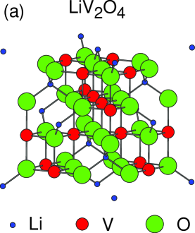
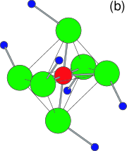
FIG. 1.: (color) (a) Normal spinel structure of LiV₂O₄ with an fcc Bravais unit cell. (b) A part of the structure depicting the trigonally distorted oxygen octahedra. The distortion shown is exaggerated for clarity and corresponds to an oxygen parameter $u=0.27$. Small, medium and large spheres represent lithium, vanadium and oxygen, respectively; their sizes have no intended physical significance.

half of the 32 octahedral holes in the oxygen sublattice per unit cell. All of the V ions are crystallographically equivalent. Due to this fact and the non-integral V oxidation state, the compound is expected to be metallic, which was confirmed by single-crystal resistivity $\rho(T)$ measurements by Rogers et al.[9] The V atoms constitute a three-dimensional network of corner-shared tetrahedra. The LiV₂ sublattice is identical to the cubic Laves phase (C15) structure, and the V sublattice is identical with the transition metal $T$ sublattice of the fcc $R_{2}T_{2}$O₇ pyrochlore structure.

Despite its metallic character, LiV₂O₄ exhibits a strongly temperature dependent magnetic susceptibility, indicating strong electron correlations. In the work reported before 1997, the observed magnetic susceptibility $\chi^{\rm obs}(T)$ was found to increase monotonically with decreasing $T$ down to $\approx$ 4 K and to approximately follow the Curie-Weiss law. [10, 11, 12, 13, 14, 15] Kessler and Sienko[10] interpreted their $\chi^{\rm obs}(T)$ data as the sum of a Curie-Weiss term $2C/(T-\theta)$ and a temperature-independent term $\chi_{0}=0.4\times 10^{-4}\,$cm³/mol. Their Curie constant $C$ was 0.468 cm³ K/(mol V), corresponding to a V⁺⁴ $g$-factor of 2.23 with spin $S=1/2$. The negative Weiss temperature $\theta=-63$ K suggests antiferromagnetic (AF) interactions between the V spins. However, no magnetic ordering was found above $4.2$ K. This may be understood in terms of possible suppression of long-range magnetic ordering due to the geometric frustration among the AF-coupled V spins in the tetrahedra network.[16, 17] Similar values of $C$ and $\theta$ have also been obtained by subsequent workers, [11, 12, 13, 14, 15] as shown in Table I, in which reported crystallographic data[18, 19, 20, 21, 22] are also shown. This local magnetic moment behavior of LiV₂O₄ is in marked contrast to the magnetic properties of isostructural LiTi₂O₄

TABLE I.: Lattice parameter $a_{0}$, oxygen parameter $u$ (see text) and magnetic parameters $\chi_{0}$, $C$ and $\theta$ reported in the literature for LiV₂O₄. The $u$ values shown are for the second setting of the space group $Fd\bar{3}m$ from the International Tables for Crystallography, Vol. A.[8] The “$T$ range” is the temperature range over which the fits to the susceptibility data were done, $\chi_{0}$ is the temperature-independent contribution, $C$ is the Curie constant and $\theta$ is the Weiss temperature. The error in the last digit of a quantity is given in parentheses. Unless otherwise noted, all measurements were done on polycrystalline samples.

$a_{0}$	$u$	$T$ range	$\chi_{0}$	$C$	$\theta$	Ref.
(Å)		(K)	$(10^{-6}\ \frac{{\rm cm}^{3}}{{\rm mol\ LiV_{2}O_{4}}})$	$(\frac{{\rm cm^{3}\ K}}{{\rm mol\ V}})$	(K)
8.22						[7]
8.2403(12)	$0.260(1)$					[18]
8.240(2)						[19]
8.22		4.2–308	37	$0.468$	$-$63	[10]
8.240(2)	$0.253(1)$					[20]
8.25a						[21]
8.255(6)	$0.260$	50–380a	37	$0.460$	$-$34	[12]
		50–380a	37	$0.471$	$-$42	[12]b
		80–300	43	$0.441\leavevmode\leavevmode\hbox{${}^{\rm a}$}$	$-$31a	[13]
8.241(3)a		80–300	43	$0.434\leavevmode\leavevmode\hbox{${}^{\rm a}$}$	$-$39a	[14]
				$0.473$		[11]
8.235		10–300	0	$0.535$	$-$35.4	[15]
8.2408(9)		100–300	230	$0.35$	$-$33	[22]

which manifests a comparatively temperature independent Pauli paramagnetism and superconductivity ($T_{\rm c}\leq 13.7$ K).[23]

Strong electron correlations in LiV₂O₄ were inferred by Fujimori et al.[24, 25] from their ultraviolet (UPS) and x-ray (XPS) photoemission spectroscopy measurements. An anomalously small density of states at the Fermi level was observed at room temperature which they attributed to the effect of long-range Coulomb interactions. They interpreted the observed spectra assuming charge fluctuations between $d^{1}$ (V⁴⁺) and $d^{2}$ (V³⁺) configurations on a time scale longer than that of photoemission ($\sim 10^{-15}$ sec). Moreover, the intra-atomic Coulomb repulsion energy, $U$, was found to be $\sim 2$ eV. This value is close to the width $W\sim 2$ eV of the $t_{2g}$ conduction band calculated for LiTi₂O₄.[26, 27] From these observations, one might infer that $U\sim W$ for LiV₂O₄, suggesting proximity to a metal-insulator transition.

We and collaborators recently reported that LiV₂O₄ samples with high magnetic purity display a crossover from the aforementioned localized moment behavior above $\sim 100$ K to a nearly temperature independent susceptibility below $\sim 30$ K.[6] This new finding was also reported independently and nearly simultaneously by two other groups.[22, 28] Specific heat measurements revealed a rapidly increasing $\gamma(T)$ with decreasing temperature below $\sim 30$ K with an exceptionally large value $\gamma(1\,{\rm K})\approx 0.42$ J/mol K².[6] To our knowledge, this $\gamma(1\,{\rm K})$ is the largest value reported for any metallic $d$-electron compound, e.g., Y_0.97Sc_0.03Mn₂ ($\lesssim 0.2$ J/mol  K²)(Ref. [29]) and V_2-yO₃ ($\lesssim 0.07$  J/mol  K²).[30] The Wilson ratio[31] at low $T$ was found to be $R_{\rm W}\sim$ 1.7, consistent with a heavy FL interpretation. From ⁷Li NMR measurements, the $T$ variation of the Knight shift $K$ was found to approxi-

mately follow that of the susceptibility. [6, 28, 32, 33, 34, 35] The ⁷Li nuclear spin-lattice relaxation rate $1/T_{1}$ in LiV₂O₄ was found to be proportional to $T$ below $\sim 4$ K, with a Korringa ratio on the order of unity, again indicating FL behavior.[6, 33, 34, 35]

In this paper we present a detailed study of the synthesis, characterization and magnetic susceptibility of LiV₂O₄. In Sec. II our synthesis method and other experimental techniques are described. Experimental results and analyses are given in Sec. III. In Sec. III A, after a brief overview of the spinel structure, we present structural characterizations of nine LiV₂O₄ samples that were prepared in slightly different ways, based upon our results of thermogravimetric analysis (TGA), x-ray diffraction measurements and their Rietveld analyses. In Sec. III B, results and analyses of magnetization measurements are given. In Sec. III B 1 an overview of the $\chi^{\rm obs}(T)\equiv M^{\rm obs}(T)/H$ data of all nine samples studied is presented. Then, in Sec. III B 2, we determine the magnetic impurity concentrations from analysis of the $M^{\rm obs}(H)$ data. Low-field ($H=10\mbox{--}100$ G) $\chi^{\rm obs}(T)$ susceptibility data, measured after zero-field cooling (ZFC) and field cooling (FC), are presented in Sec. III B 3 a, from which we infer that spin-glass ordering does not occur above 2 K. The above determinations of magnetic impurity contributions to $M^{\rm obs}(H,T)$ allow us to extract the intrinsic susceptibility $\chi(T)$ from $\chi^{\rm obs}(T)$, as explained in Sec. III B 3 b. The paramagnetic orbital Van Vleck susceptibility $\chi^{\rm VV}$ contribution is determined in Sec. IV A from a so-called $K$-$\chi$ analysis using ⁵¹V NMR measurements.[32, 35] We attempt to interpret the $\chi(T)$ data using three theories. First, the predictions of high temperature series expansion (HTSE) calculations for the spin $S=1/2$ Heisenberg model are compared to our $\chi(T)$ data in Sec. IV B. Second, a crystalline electric field theory prediction with the assumption of cubic point symmetry of the vanadium ion is tested in Sec. IV C. Third, we test the applicability of the Kondo and Coqblin-Schrieffer models to our $\chi(T)$ data in Sec. IV D. A summary and discussion are given in Sec. V. Throughout this paper, a “mol” means a mole

TABLE II.: Results of Rietveld refinements of x-ray diffraction measurements and magnetization $M^{\rm obs}(H)$ isotherm analyses. The oxygen parameter ($u$) is for the second setting of the space group $Fd\bar{3}m$ from the International Tables for Crystallography, Vol. A.[8] $f_{\rm str~{}imp}$ is the impurity concentration. The error in the last digit of a quantity is given in parentheses. The detection limit of $f_{\rm str~{}imp}$ is assumed to be 1%.[38] For samples 3 and 7 in which no discernable impurities were seen, this detection limit is listed; the Rietveld refinement for sample 5 directly yielded $f_{\rm str~{}imp}<1$%.

Sample	Alt. Sample	Cooling	Impurity	$a_{0}$	$u$	$f_{\rm str~{}imp}$
No.	No.			(Å)		(mol %)
1	4-0-1	air	V3O5	8.24062(11)	0.26115(17)	2.01
2	3-3	air	V2O3	8.23997(4)	0.2612(20)	1.83
3	4-E-2	air	pure	8.24100(15)	0.26032(99)	$<1$
4	3-3-q1	LN2	V3O5	8.24622(23)	0.26179(36)	3.83
4A	3-3-q2	ice H2O	V2O3	8.24705(29)	0.26198(39)	1.71
4B	3-3-a2	slow cool	V2O3	8.24734(20)	0.26106(32)	1.46
5	6-1	air	V2O3	8.24347(25)	0.26149(39)	$<1$
6	12-1	air	V3O5	8.23854(11)	0.26087(23)	2.20
7	13-1	air	pure	8.24114(9)	0.26182(19)	$<1$

of LiV₂O₄ formula units, unless otherwise noted.

II Synthesis and Experimental Details

Polycrystalline samples of LiV₂O₄ were prepared using conventional solid-state reaction techniques with two slightly different paths to the products. The five samples used in our previous work[6] (samples 1 through 5) were prepared by the method in Ref. [23]. Two additional samples (samples 6 and 7) were synthesized by the method of Ueda et al.[22] Different precursors are used in the two methods: “Li₂VO_3.5” (see below) and Li₃VO₄, respectively. Both methods successfully yielded high quality LiV₂O₄ samples which showed the broad peak in $\chi^{\rm obs}(T)$ at $\approx 16$ K. In this report, only the first synthesis method is explained in detail, and the reader is referred to Ref. [22] for details of the second method.

The starting materials were Li₂CO₃ (99.999 %, Johnson Matthey), V₂O₃, and V₂O₅ (99.995 %, Johnson Matthey). Oxygen vacancies tend to be present in commercially obtained V₂O₅.[36] Therefore, the V₂O₅ was heated in an oxygen stream at 500-550 ^∘C in order to fully oxidize and also dry it. V₂O₃ was made by reduction of either V₂O₅ or NH₄VO₃ (99.995 %, Johnson Matthey) in a tube furnace under 5 % H₂/95 % He gas flow. The heating was done in two steps: at 635 ^∘C for $\approx 1$  day and then at 900–1000 ^∘C for up to 3 days. The oxygen content of the nominal V_2-yO₃ obtained was then determined by thermogravimeteric analysis (TGA, see below). The precursor “Li₂VO_3.5” (found to be a mixture of Li₃VO₄ and LiVO₃ from an x-ray diffraction measurement) was prepared by heating a mixture of Li₂CO₃ and V₂O₅ in a tube furnace under an oxygen stream at $\approx 525$ ^∘C until the expected weight decrease due to the loss of carbon dioxide was obtained. Ideally the molar ratio of Li₂CO₃ to V₂O₅ for the nominal composition Li₂VO_3.5 is 2 to 1. A slight adjustment was, however, made to this ratio according to the actual measured oxygen content of the V_2-yO₃ ($y\simeq 0.005$ to 0.017) so that the final product

is stoichiometric LiV₂O₄. This precursor and V_2-yO₃ were ground thoroughly inside a helium-filled glovebox. The mixture was then pelletized, wrapped in a piece of gold foil, sealed into a quartz tube under vacuum, and heated between 570 ^∘C and 700 ^∘C for $\lesssim 2$  weeks. The as-prepared samples were all removed from the oven at the final furnace temperature and air-cooled to room temperature. For samples 2 and 3 additional heating at a higher $T=750$ ^∘C was given, with a repeated sequence of grinding, repelletizing and reheating for sample 2. From $\approx 725$ ^∘C different methods of cooling, liquid-nitrogen or ice-water quenching or slow-oven cooling, were applied to pieces from sample 2, yielding samples 4, 4A and 4B, respectively.

Using a Rigaku Geigerflex diffractometer with a curved graphite crystal monochrometer, x-ray diffraction patterns were obtained at room temperature with Cu K$\alpha$ radiation. Rietveld analyses of the diffraction patterns were carried out using the angle-dispersive x-ray diffraction version of the RIETAN-97$\beta$ program.[37, 38]

TGA measurements were done using a Perkin-Elmer TGA 7 Thermogravimetric Analyzer. Oxygen contents of the samples were calculated from weight gains after heating in an oxygen flow to 540 ^∘C for LiV₂O₄ and 620 ^∘C for V_2-yO₃, assuming that the oxidized products contained vanadium as V⁺⁵.

Magnetization $M^{\rm obs}$ measurements were performed using a Quantum Design MPMS5 superconducting quantum interference device (SQUID) magnetometer over the $T$ range from 1.8–2 K to 400 K with $H$ up to 5.5 T. Zero-field-cooled (ZFC, usually obtained by quenching the superconducting solenoid) $M^{\rm obs}(H=1\,{\rm T},T)$ scans were carried out and isothermal $M^{\rm obs}(H)$ data at various temperatures were obtained. Low-field (10–100 G) ZFC and field-cooled (FC) $M(T)$ scans were done from 1.8–2 K to 50 K in order to check for the presence or absence of spin-glass ordering.

III Results and Analyses

A Structure

X-ray diffraction patterns of our nine LiV₂O₄ samples revealed that the samples were single-phase or very nearly so. Figure 2(a) shows the diffraction pattern of sample 7 which has no detectable impurities. The nine samples described in detail in this paper are categorized into three groups in terms of purity: essentially impurity-free (samples 3 and 7), V₃O₅ impurity (samples 1, 4 and 6) and V₂O₃ impurity (samples 2, 4A, 4B and 5). The presence of these impurity phases is detected in magnified views of the diffraction patterns as shown in Fig. 2(b). Results from Rietveld analyses of the diffraction patterns for these samples are given in Table II. The refinements of the spinel phase (space group $Fd\bar{3}m$, No. 227) were based on the assumption of exact LiV₂O₄ stoichiometry and the normal-spinel structure cation distribution. The values of the isotropic thermal-displacement parameters $B$ of lithium and oxygen were taken from the Rietveld analysis of neutron diffraction measurements on our LiV₂O₄ sample 5 by Chmaissem et al.,[39] and fixed throughout to $B_{\rm Li}=1.1$ Å and $B_{\rm O}=0.48$ Å, respectively. These two atoms do not scatter x-rays strongly enough to allow accurate determinations of the $B$ values from Rietveld refinements of our x-ray diffraction data.

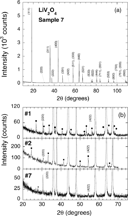
FIG. 2.: (a) X-ray diffraction pattern of LiV₂O₄ sample 7. The spinel-phase peaks are indexed as shown. (b) Expanded plots of the X-ray patterns of samples 1 (top), 2 (middle) and 7 (bottom). Indexed peaks are those of the spinel phase. Sample 1 has V₃O₅ impurity (filled circles), whereas sample 2 has V₂O₃ impurity (filled squares). Sample 7 has no impurity peaks except possibly the very weak unidentified one marked with a star.

The positions of the oxygen atoms within the unit cell of the spinel structure are described by a variable oxygen parameter $u$ associated with the $32e$ positions in space group $Fd\bar{3}m$. The value of $u$ [in the space group setting with the origin at center ($\bar{3}m$)] for each of our samples was found to be larger than the ideal close-packed-oxygen value of 1/4. Compared to the “ideal” structure with $u=1/4$, the volumes of an oxygen tetrahedron and an octahedron become larger and smaller, respectively. The increase of the tetrahedron volume takes place in such a way that each of the four Li-O bonds are lengthened along one of the $<$111$>$ directions, so that the tetrahedron remains undistorted. As a result of this elongation, the tetrahedral and octahedral holes become respectively larger and smaller.[40] Each of the oxygen atoms in a tetrahedron is also bonded to three V atoms. Since the fractional coordinates of both Li and V are fixed in terms of the unit cell edge, an oxygen octahedron centered by a V atom is accordingly trigonally distorted. This distortion is illustrated in Fig. 1(b).

The nine LiV₂O₄ samples were given three different heat treatments after heating to 700 to 750 ^∘C: air-cooling (samples 1, 2, 3, 5, 6 and 7), liquid-nitrogen quenching (sample 4), ice-water quenching (sample 4A) or oven-slow cooling at $\approx 20\,^{\circ}$C/hr (sample 4B). Possible loss of Li at the high synthesis temperature, perhaps in the form of a lithium oxide, was a concern. In a detailed neutron diffraction study, Dalton et al.[41] determined the lithium contents in their samples of Li_1+xTi_2-xO₄ ($0\leq x\leq 0.33$), and found lithium deficiency in the $8a$ site of the spinel phase of all four samples studied. If the spinel phase in the Li-V-O system is similarly Li-deficient, then samples of exact stoichiometry LiV₂O₄ would contain V-O impurity phase(s), which might then explain the presence of small amounts of V₂O₃ or V₃O₅ impurity phases in most of our samples.

Sample 3 was intentionally made slightly off- stoichiometric, with the nominal composition LiV_1.92O_3.89. A TGA measurement in oxygen showed a weight gain of 12.804 % to the maximally oxidized state. If one assumes an actual initial composition LiV_1.92O_3.89+δ, this weight gain corresponds to $\delta=0.08$ and an actual initial composition of LiV_1.92O_3.97 which can be rewritten as Li_1.01V_1.93O₄ assuming no oxygen vacancies on the oxygen sublattice. On the other hand, if one assumes an actual initial composition of Li_1-xV_1.92O_3.89, then the weight gain yields $x=0.19$, and an initial composition Li_0.81V_1.92O_3.89 which can be similarly rewritten as Li_0.83V_1.97O₄. Our Rietveld refinements could not distinguish these possibilities from the stoichiometric composition Li[V₂]O₄ for the spinel phase.

Sample 4, which was given a liquid-nitrogen quench from the final heating temperature of $\simeq 725\,^{\circ}$C (labelled “LN₂” in Table II), is one of the structurally least pure samples (see Table II). Our Rietveld refinement of the x-ray diffraction pattern for this sample did not reveal any discernable deviation of the cation occupancy from that of ideal Li[V₂]O₄. There is a strong similarity among samples 4, 4A (ice-water quenched) and 4B (oven-slow cooled), despite their different heat treatments. These samples all have much larger lattice parameters ($a_{0}\gtrsim 8.246$ Å) than the other samples. The as-prepared sample 2, from which all three samples 4, 4A and 4B were obtained by the above quenching heat treatments, has a much smaller lattice parameter. On the other hand, the oxygen parameters $u$ of these four samples are similar to each other and to those of the other samples in Table II.

The weight gains on oxidizing our samples in oxygen in the TGA can be converted to values of the average oxidation state per vanadium atom, assuming the ideal stoichiometry LiV₂O₄ for the initial composition. The values, to an accuracy of $\pm 0.01$, are 3.57, 3.55, 3.60, 3.56, 3.56, 3.57, 3.57, 3.55 for samples 1–7 and 4B, respectively. This measurement was not done for sample 4A. These values are systematically higher than the expected value of 3.50, possibly because the samples were not completely oxidized. Indeed, the oxidized products were gray-black, and upon crushing were brown, rather than a light color. On the other hand, x-ray diffraction patterns of the “LiV₂O_5.5” oxidation products showed only a mixture of LiVO₃ and Li₄V₁₀O₂₇ phases as expected from the known Li₂O-V₂O₅ phase diagram.[42] Our upper temperature limit (540^∘C) during oxidation of the LiV₂O₄ samples was chosen to be low enough so that the oxidized product at that temperature contained no liquid phase; this temperature may have been too low for complete oxidation to occur. In contrast, our V_2-yO₃ starting materials turned orange on oxidation, which is the same color as the V₂O₅ from which they were made by hydrogen reduction.

B Magnetization Measurements

1 Overview of Observed Magnetic Susceptibility

An overview of the observed ZFC magnetic susceptibilities $\chi^{\rm obs}(T)\equiv M^{\rm obs}(T)/H$ at $H=1.0$ T from 1.8–2 K to 400 K of the nine LiV₂O₄ samples is shown in Figs. 3 (a), (b) and (c). The $\chi^{\rm obs}(T)$ data for the various samples show very similar Curie-Weiss-like behavior for $T\gtrsim 50$ K. Differences in $\chi^{\rm obs}(T)$ between the samples appear at lower $T$, where variable Curie-like $C_{\rm imp}/T$ upturns occur.

Samples 1 and 6 clearly exhibit shallow broad peaks in $\chi^{\rm obs}$ at $T\approx 16$ K. The $\chi^{\rm obs}(T)$ of sample 6 is systematically slightly larger than that of sample 1; the reason for this shift is not known. Samples 3 and 4 also show the broad peak with a relatively small Curie-like upturn. Samples 2 and 7 show some evidence of the broad peak but the peak is partially masked by the upturn. For samples 4A, 4B and 5, the broad peak is evidently masked by larger Curie impurity contributions. From Fig. 3 and Table II, the samples 1, 4 and 6 with the smallest Curie-like magnetic impurity contributions contain V₃O₅ impurities, whereas the other samples, with larger magnetic impurity contributions, contain V₂O₃ impurities. The reason for this correlation is not clear. The presence of the vanadium oxide impurities by itself should not be a direct cause of the Curie-like upturns. The susceptibility of pure V₂O₃ follows the Curie-Weiss law in the metallic $T$ region above $\sim 170$ K, but for $T\lesssim 170$ K it becomes an antiferromagnetic insulator, showing a decrease in

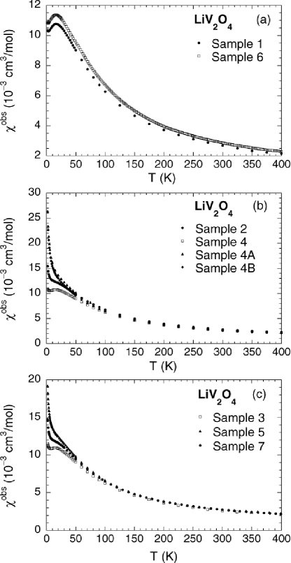
FIG. 3.: Observed magnetic susceptibility $\chi^{\rm obs}(T)$ ($\equiv M^{\rm obs}/H$) of all the nine samples studied, measured with $H=1$ T after being zero-field cooled to the lowest $T$: (a) Samples 1 and 6; (b) samples 2, 4, 4A and 4B; (c) samples 3, 5 and 7.

$\chi(T)$.[43] V_2-yO₃ ($y\approx 0.03$), on the other hand, sustains its high-$T$ metallic state down to low temperatures, and at its Néel temperature $T_{\rm N}\sim 10$ K it undergoes a transition to an antiferromagnetic phase with a cusp in $\chi(T)$.[43] V₃O₅ also orders antiferromagnetically at $T_{\rm N}=75.5$ K, but $\chi(T)$ shows a broad maximum at a higher $T=125$ K.[44] Though not detected in our x-ray diffraction measurements, V₄O₇, which has the same V oxidation state as in LiV₂O₄, also displays a cusp in $\chi^{\rm obs}(T)$ at $T_{\rm N}\approx 33$ K and $\chi^{\rm obs}(T)$ follows the Curie-Weiss law for $T\gtrsim 50$ K.[44] The susceptibilities of these V-O phases are all on the order of $10^{-4}$ to $10^{-3}$ cm³/mol at low $T$.[43, 44] Moreover, the $T$ variations of $\chi^{\rm obs}(T)$ in these vanadium oxides for $T\lesssim 10$ K are, upon decreasing $T$, decreasing (V_2-yO₃) or nearly $T$ independent (V₃O₅ and V₄O₇), in contrast to the increasing behavior of our Curie-like impurity susceptibilities. From the above discussion and the very small amounts of V-O impurity phases found from the Rietveld refinements of our x-ray diffraction measurements, we conclude that the V-O impurity phases cannot give rise to the observed Curie-like upturns in our $\chi^{\rm obs}(T)$ data at low $T$. These Curie-like terms therefore most likely arise from paramagnetic defects in the spinel phase and/or from a very small concentration of an unobserved impurity phase.

Figure 3(b) shows how the additional heat treatments of the as-prepared sample 2 yield different behaviors of $\chi^{\rm obs}(T)$ at low $T$ in samples 4, 4A and 4B. Only liquid-nitrogen quenching (sample 4) caused a decrease in the Curie-like upturn of sample 2. On the contrary, ice water quenching (sample 4A) and oven-slow cooling (sample 4B) caused $\chi^{\rm obs}(T)$ to have an even larger upturn. However, the size of the Curie-like upturn in $\chi^{\rm obs}(T)$ of sample 4 was found to be irreproducible when the same liquid-nitrogen quenching procedure was applied to another piece from sample 2; in this case the Curie-like upturn was larger, not smaller, than in sample 2. The observed susceptibility (not shown) of this latter liquid nitrogen-quenched sample is very similar to those of samples 4A and 4B. The $\chi^{\rm obs}(T)$ of samples 4A and 4B resemble those reported previously. [10, 11, 12, 13, 14, 15]

2 Isothermal Magnetization versus Magnetic Field

Larger Curie-like upturns were found in samples with larger curvatures in the isothermal $M^{\rm obs}(H)$ data at low $T$. A few representative $M^{\rm obs}(H,2\,{\rm K})$ data for samples showing various extents of curvatures in $M^{\rm obs}(H)$ are shown in Fig. 4, which may be compared with the corresponding $\chi^{\rm obs}(T)$ data at low $T$ in Figs. 3. This correlation suggests that the Curie-like upturns in $\chi^{\rm obs}(T)$ arise from paramagnetic (field-saturable) impurities/defects in the samples. On the other hand, there is no obvious correlation between the magnetic impurity concentration and the V₂O₃ or V₃O₅ phase impurity concentration, as noted above.

The isothermal $M^{\rm obs}(H)$ data for $H\leq 5.5$ T displayed negative curvature for $T\lesssim 10$–20 K and linear behavior for higher $T$, as illustrated for sample 1 in Fig. 5. The concentrations and other parameters of the magnetic impurities in the various samples were obtained from analyses of $M^{\rm obs}(H)$ isotherms as follows. From high-field measurements, the intrinsic magnetization $M(H,0.5\,{\rm K})$ of LiV₂O₄ is proportional to $H$ up to $H\sim$ 16 T.[45] Therefore, the observed molar magnetization $M^{\rm obs}(H,T)$ isotherm data for each sample were fitted by the equation

$$M^{\rm obs}(H,T)\ =M_{\rm imp}(H,T)+M(H,T)$$ (2)

$$=f_{\rm imp}N_{\rm A}g_{\rm imp}\mu_{\rm B}S_{\rm imp}B_{S_{\rm imp}}(x)+\chi(T)H~{},$$

FIG. 4.: Comparison of the negative curvatures of observed magnetization isotherms $M^{\rm obs}$ at $T=2$ K versus applied magnetic field $H$ for samples 1, 3, 5 and 7.

FIG. 5.: Observed magnetization $M^{\rm obs}$ versus applied magnetic field $H$ isotherms at temperatures $T=$ 2, 10 and 300 K for LiV₂O₄ sample 1. Negative curvature in $M^{\rm obs}(H)$ is not present for $T>10$ K for this sample.

where $f_{\rm imp}$ is the magnetic impurity concentration, $N_{\rm A}$ Avogadro’s number, $g_{\rm imp}$ the impurity $g$-factor, $\mu_{\rm B}$ the Bohr magneton, $S_{\rm imp}$ the impurity spin, $B_{S_{\rm imp}}$ the Brillouin function, $\chi$ the intrinsic susceptibility of the LiV₂O₄ spinel phase and $H$ the applied magnetic field. The argument of the Brillouin function is $x=g_{\rm imp}\mu_{\rm B}S_{\rm imp}H/[k_{\rm B}(T-\theta_{\rm imp})]$. $\theta_{\rm imp}$ represents the Weiss temperature of the Curie-Weiss law when the susceptibility is obtained by expanding the Brillouin function in the limit of small $H/(T-\theta_{\rm imp})$. Incorporating the parameter $\theta_{\rm imp}\neq 0$ takes account of possible interactions between magnetic impurities in a mean-field manner. To improve the precision of the obtained fitting parameters, we fitted $M^{\rm obs}(H)$ isotherm data measured at more than one low temperature simultaneously by Eq. (LABEL:MEq). Since the negative curvature of the isothermal $M^{\rm obs}(H,T)$ data diminishes rapidly with increasing $T$, only low $T$ (1.8–6 K) data were used. Furthermore, a linear $T$ dependence of $\chi(T)$ in this $T$ range was assumed [see Fig. 3(a)] in order to reduce the number of free parameters. However, $\chi(T=2\,{\rm K})$ and the linear slope d$\chi$/d$T$ still have to be determined. Hence up to six free parameters were to be determined by fitting Eq. (LABEL:MEq) to the data: $f_{\rm imp}$, $g_{\rm imp}$, $S_{\rm imp}$, $\theta_{\rm imp}$, $\chi(T=2\,{\rm K})$ and d$\chi$/d$T$.

With all six parameters varied as free parameters, fits of $M^{\rm obs}(H,T)$ by Eq. (LABEL:MEq) produced unsatisfactory results, yielding parameters with very large estimated standard deviations. Therefore, we fixed $S_{\rm imp}$ to various half-integer values starting from 1/2, thereby reducing the number of free parameters of each fit to five. With regard to the $g_{\rm imp}$ values, $g$-factors of slightly less than 2 are observed in V⁺⁴ compounds: VO₂ (1.964) (Ref. [46]), (NH₄)_xV₂O₅ (1.962) (Ref. [47]) and Li_xV₂O₅ (1.96).[48] Using $g_{\rm imp}\approx 2$ as a guide, we selected a few values of $S_{\rm imp}$ which resulted in $g\sim 2$ in the five-parameter fit. Then using the obtained parameter values we calculated and plotted the impurity magnetization $M_{\rm imp}$ ($\equiv M^{\rm obs}-\chi H$) versus $H/(T-\theta_{\rm imp})$ for all the low $T$ data utilized in the fit by Eq. (LABEL:MEq). If a fit is valid, then all the $M_{\rm imp}[H/(T-\theta_{\rm imp})]$ data points obtained at the various isothermal temperatures for each sample should collapse onto a universal curve described by $M_{\rm imp}=f_{\rm imp}N_{\rm A}g_{\rm imp}\mu_{\rm B}S_{\rm imp}B_{S_{\rm imp}}(x)$. The fixed value of $S_{\rm imp}$ which gave the best universal behavior for a given sample was chosen. Then, using this $S_{\rm imp}$, we fixed the value of $g_{\rm imp}$ to 2 to see if the resultant $M_{\rm imp}[H/(T-\theta_{\rm imp})]$ data yielded a similar universal behavior. For the purpose of reducing the number of free parameters as much as possible, if this fixed-$g$ fit did yield a comparable result, the parameters obtained were taken as the final fitting parameters and are reported in this paper. For sample 1 only, the fit parameters obtained by further fixing $\theta_{\rm imp}=0$ are reported here. To estimate the goodness of a fit, the $\chi^{2}$ per degree of freedom (DOF) was obtained, which is defined as $(N_{\rm p}-P)^{-1}\sum_{i=1}^{N_{\rm p}}(M_{i}-M_{i}^{\rm calc})^{2}/\sigma_{i}^{2}$, where $N_{p}$ is the number of data points, $P$ is the number of free parameters, and $\sigma_{i}$ is the standard deviation of the observed value $M_{i}$. A fit is regarded as satisfactory if $\chi^{2}/{\rm DOF}\lesssim 1$, and this criterion was achieved for each of the nine samples.

The magnetic parameters for each sample, obtained as described above, are listed in Table III. Plots of $M_{\rm imp}$ versus $H/(T-\theta_{\rm imp})$ for the nine samples are given in Figs. 6(a), (b) and (c), where an excellent universal behavior for each sample at different temperatures is seen. The two magnetically purest samples 1 and 6 have the largest relative deviations of the data from the respective fit curves, especially at the larger values of $H/(T-\theta_{\rm imp})$.

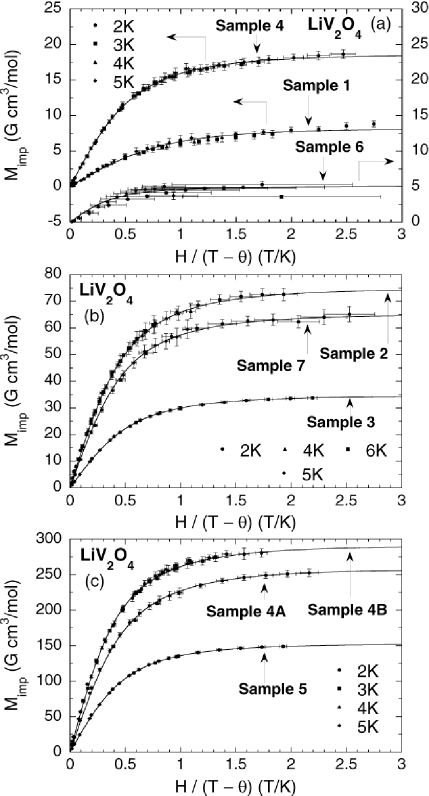
FIG. 6.: Calculated impurity magnetizations $M_{\rm imp}\equiv$ $M^{\rm obs}-\chi H$ versus $H/(T-\theta_{\rm imp})$ for the nine LiV₂O₄ samples. For each sample, the solid curve is the best-fit Brillouin function Eq. (LABEL:MEq).

TABLE III.: Results of magnetization $M^{\rm obs}(H,T)$ isotherm analyses, where the $T$ values used are listed in the second column. $f_{\rm mag~{}imp}$ is the molar magnetic impurity concentration. The error in the last digit of a quantity is given in parentheses. All numbers without an error listed were fixed in the fit. The Curie constant of the impurities was calculated from $C_{\rm imp}=f_{\rm mag~{}imp}N_{\rm A}g^{2}_{\rm imp}\mu^{2}_{\rm B}S_{\rm imp}(S_{\rm imp}+1)/(3k_{\rm B})$.

Sample	$T$	$S_{\rm imp}$	$g_{\rm imp}$	$\theta_{\rm imp}$	$f_{\rm mag~{}imp}$	$C_{\rm imp}$	$\chi(2\,{\rm K})$	$d\chi/dT$
No.	(K)	(fixed)		(K)	(mol %)	($10^{-3}$ $\frac{{\rm cm}^{3}\,{\rm K}}{{\rm mol}}$)	($10^{-2}$ $\frac{{\rm cm}^{3}}{{\rm mol}}$)	($\frac{{\rm cm}^{3}}{{\rm mol\,K}}$)
1	2,3,4,5	3/2	2	0	0.049(2)	0.74	1.026(1)	7.3(1)
2	2,4,6	3	2.00(6)	$-$0.6(2)	0.22(1)	13	1.034(5)	6.7(4)
3	2,5	5/2	2.10(2)	$-$0.51(5)	0.118(2)	4.9	0.9979(6)	7.46(7)
4	2,3,4,5	5/2	2	$-$0.2(1)	0.066(2)	2.5	0.9909(9)	6.7(1)
4A	2,5	3	2	$-$0.5(1)	0.77(2)	46	1.145(9)	6.5(9)
4B	2,3,4,5	7/2	2	$-$1.2(1)	0.74(2)	52	1.13(1)	4.4(7)
5	2,5	5/2	2.31(3)	$-$0.59(4)	0.472(8)	24	1.091(2)	5(3)
6	2,5	4	2	$-$0.9(14)	0.0113(6)	1.1	1.067	5.6(2)
7	2,5	3	2	$-$0.2(2)	0.194(7)	12	1.094(4)	5.4(4)

Since these two samples contain extremely small amounts of paramagnetic saturable impurities, the magnetic parameters of the impurities could not be determined to high precision. The impurity spins $S_{\rm imp}$ obtained for the nine samples vary from 3/2 to 4. In general, the magnetic impurity Weiss temperature $|\theta_{\rm imp}|$ increased with magnetic impurity concentration $f_{\rm imp}$. From the chemi- cal analyses of the starting materials (V₂O₅, NH₄VO₃ and Li₂CO₃) supplied by the manufacturer, magnetic impurity concentrations of 0.0024 mol % Cr and 0.0033 mol % Fe are inferred with respect to a mole of LiV₂O₄, which are too small to account for the paramagnetic impurity concentrations we derived for our samples.

3 Magnetization versus Temperature Measurements

a Low Magnetic Field ZFC and FC Measurements

The zero-field-cooled (ZFC) $\chi^{\rm obs}(T)$ data in Fig. 3(a) for our highest magnetic purity samples 1 and 6 show a broad maximum at $T^{\rm peak}\approx 16$ K. One interpretation might be that static short-range (spin-glass) ordering sets in below this temperature. To check for spin-glass ordering, we carried out low-field (10–100 G) ZFC and field-cooled (FC) magnetization measurements from 1.8–2 K to 50 K on all samples except samples 2 and 4B. For each sample, there was no hysteresis between the ZFC and FC measurements, as illustrated for sample 4 in Fig. 7, and thus no evidence for spin-glass ordering above 1.8–2 K.[49]

Ueda et al.[22] reported that spin-glass ordering occurs in the zinc-doped lithium vanadium oxide spinel Li_1-xZn_xV₂O₄ for $0.1<x\leq 0.9$ . However, spin-glass ordering was not seen in the pure compound LiV₂O₄, consistent with our results. Further, positive-muon spin relaxation $\mu$SR measurements for sample 1 did not detect static magnetic ordering down to 20 mK.[6] However, the $\mu$SR measurements did indicate the presence of static spin-glass ordering in the off-stoichiometric sample 3 below 0.8 K.[6] As mentioned in Sec. III A, the stoichiometry of sample 3 was intentionally made slightly cation-

FIG. 7.: Observed magnetic susceptibility $\chi^{\rm obs}(T)\equiv$ $M^{\rm obs}(T)/H$ versus temperature $T$ in a low magnetic field $H=50$ G of LiV₂O₄ sample 4 cooled in zero field (ZFC) and in the low field (FC).

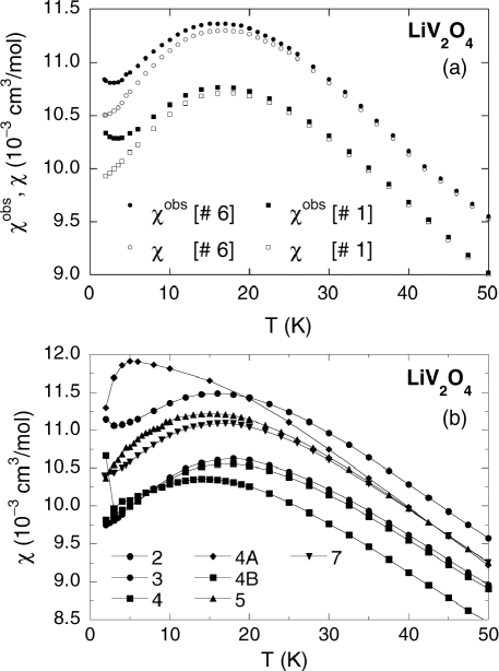
FIG. 8.: Observed susceptibilities $\chi^{\rm obs}$ and derived intrinsic susceptibilities $\chi$ versus temperature $T$ of (a) samples 1 and 6 and (b) samples 2, 3, 4, 5, 7, 4A and 4B. The solid lines are guides to the eye.

deficient, and may contain cation vacancies. Such a defective structure could facilitate the occurrence of the spin-glass behavior by relieving the geometric frustration among the V spins. Whether the nature of the spin-glass ordering in sample 3 is similar to or different from that in Li_1-xZn_xV₂O₄ noted above is at present unclear.

b Intrinsic Susceptibility

The intrinsic susceptibility $\chi(T)$ was derived from the observed $M^{\rm obs}(T)$ data at fixed $H=$ 1 T using $\chi(T)=[M^{\rm obs}(T)-M_{\rm imp}(H,T)]/H$, where $M_{\rm imp}(H,T)$ is given by Eq. (LABEL:MEq) with $H=1$ T and by the parameters for each sample given in Table III, and $T$ is the only variable. The $\chi(T)$ for each of the nine samples is shown in Figs. 8(a) and (b), along with $\chi^{\rm obs}(T)$ for samples 1 and 6. A shallow broad peak in $\chi(T)$ is seen at a temperature $T_{\rm peak}=18,16,18,18,15,17,17,5$ and 14 K for samples 1–7, 4A and 4B, respectively. The peak profiles seen in $\chi(T)$ for the two magnetically purest samples 1 and 6 are regarded as most closely reflecting the intrinsic susceptibility of LiV₂O₄. This peak shape is obtained in the derived $\chi(T)$ of all the samples except for sample 4A, as seen in Fig. 8(b). The physical nature of the magnetic impurities in sample 4A is evidently different from that in the other samples. Except for the anomalous sample 4A, the $\chi(T=0)$ values were estimated from Figs. 8(a) and (b), neglecting the small residual increases at the lowest $T$ for samples 2, 6, 7 and 4B, to be

$$\chi(0)= 9.8 ,~{}10.8,~{}9.6,~{}9.7,~{}10.0,~{}10.2,~{}10.2,~{}$$ (4)

$$9.8 \times 10^{-3}\,{\rm cm^{3}/mol}~{}~{}(\mbox{samples~{}1--7,~{}4B})~{}~{}.$$ (5)

IV Modeling of the Intrinsic Magnetic Susceptibility

A The Van Vleck Susceptibility

The Van Vleck paramagnetic orbital susceptibility $\chi^{\rm VV}$ may be obtained in favorable cases from the so-called $K$-$\chi$ analysis, i.e., if the transition metal NMR frequency shift $K$ depends linearly on $\chi$, with $T$ an implicit parameter. One decomposes $\chi(T)$ per mole of transition metal atoms according to $\chi(T)=\chi^{\rm core}+\chi^{\rm VV}+\chi^{\rm spin}(T)$. We neglect the diamagnetic orbital Landau susceptibility, which should be small for $d$-electron bands.[50] The NMR shift is written in an analogous fashion as

$$K(T)=K^{\rm VV}+K^{\rm spin}(T)~{}~{};$$ (6)

a term $K^{\rm core}$ does not appear on the right-hand side of Eq. (6) because the absolute shift due to $\chi^{\rm core}$ is expected to be about the same as in the Knight shift reference compound and hence does not appear in the shift measured with respect to the reference compound. Each component of $K$ is written as a product of the corresponding component of $\chi$ and of the hyperfine coupling constant $A$ as

$$K^{\rm VV} = \frac{A^{\rm VV}}{N_{\rm A}\mu_{\rm B}}\chi^{\rm VV}~{}~{},$$ (8)

$$K^{\rm spin} = \frac{A^{\rm spin}}{N_{\rm A}\mu_{\rm B}}\chi^{\rm spin}~{}~{}.$$ (9)

Combining Eqs. (6) and (6) yields

$$K=\frac{A^{\rm VV}}{N_{\rm A}\mu_{\rm B}}\chi^{\rm VV}+\frac{A^{\rm spin}}{N_{\rm A}\mu_{\rm B}}\chi^{\rm spin}~{}~{}.$$ (10)

If $K(T)$ varies linearly with $\chi(T)$, then the slope is $A^{\rm spin}/N_{\rm A}\mu_{\rm B}$ since $\chi^{\rm VV}$ (and $\chi^{\rm core}$) is normally independent of $T$. We write the observed linear relation as

$$K=K_{o}+\frac{A^{\rm spin}}{N_{\rm A}\mu_{\rm B}}\chi~{}~{}.$$ (11)

Setting the right-hand-sides of Eqs. (10) and (11) equal to each other gives

$$\chi^{\rm VV}=\frac{N_{\rm A}\mu_{\rm B}K_{o}+A^{\rm spin}\chi^{\rm core}}{A^{\rm VV}-A^{\rm spin}}~{}~{}.$$ (12)

FIG. 9.: ⁵¹V NMR Knight shift $K$ versus observed magnetic susceptibility $\chi^{\rm obs}$ for LiV₂O₄ by Amako et al.[13, 32] and by Mahajan et al.[35] for LiV₂O₄ sample 2. The lines are linear fits to the data according to Eq. (13).

From ⁵¹V NMR and $\chi(T)$ measurements, the $K$ vs. $\chi$ relationship for LiV₂O₄ was determined by Amako et al.[32] and was found to be linear from 100–300 K, as shown in Fig. 9. Our fit to their data gave

$$K=0.0117(4)-\biggl{[}17.08(21)\,{\rm\frac{mol\,V}{cm^{3}}}\biggr{]}\chi\biggl{(}{\rm\frac{cm^{3}}{mol\,V}}\biggr{)}~{}~{},$$ (13)

shown as the straight line in Fig. 9. Comparison of Eqs. (11) and (13) yields

$$K_{o}=0.0117(4)~{}~{},$$ (15)

$$A^{\rm spin}=-95.4(12)\,{\rm kG}~{}~{}.$$ (16)

The orbital Van Vleck hyperfine coupling constants for V⁺³ and V⁺⁴ are similar. For atomic V⁺³, one has $A^{\rm VV}=403$ kG (Ref. [51]). We will assume that $A^{\rm VV}$ in LiV₂O₄ is given by that[52] for atomic V⁺⁴,

$$A^{\rm VV}=455\,{\rm kG}~{}~{}.$$ (17)

The core susceptibility is estimated here from Selwood’s table,[53] using the contributions [in units of $-10^{-6}$ cm³/(mol ion)] 1 for Li⁺¹, 7 for V⁺⁴ and 12 for O^-2, to be

$$\chi^{\rm core}=-63\times 10^{-6}\,\frac{{\rm cm^{3}}}{{\rm mol}}~{}~{}.$$ (18)

Inserting Eqs. (13)–(18) into (12) yields

$$\chi^{\rm VV}=2.48(9)\times 10^{-4}\,\frac{{\rm cm^{3}}}{{\rm mol}}~{}~{}.$$ (19)

Mahajan et al.[35] have measured the ⁵¹V $K(T)$ for our LiV₂O₄ sample 2 from 78 to 575 K. Their data are plotted versus our measurement of $\chi^{\rm obs}(T)$ for sample 2 from 74 to 400 K in Fig. 9. Applying the same $K$-$\chi$ analysis as above, we obtain

$$K_{o}=0.0101(3)~{}~{},$$ (20)

$$A^{\rm spin}=-76.9(8)\,{\rm kG}~{}~{},$$ (21)

$$\chi^{\rm VV}=2.22(6)\times 10^{-4}\,\frac{{\rm cm^{3}}}{{\rm mol}}~{}~{},$$ (22)

where the linear fit of $K$ vs. $\chi^{\rm obs}$ is shown by the dashed line in Fig. 9.

We may compare our similar values of $\chi^{\rm VV}$ for LiV₂O₄ in Eqs. (19) and (22) with those obtained from $K$-$\chi$ analyses of other oxides containing V⁺³ and V⁺⁴. For stoichiometric V₂O₃ above its metal-insulator transition temperature of $\sim 160$ K, Jones[54] and Takigawa et al.[51] respectively obtained $\chi^{\rm VV}=2.10$ and $2.01\times 10^{-4}$ cm³/(mol V). Kikuchi et al.[55] obtained $\chi^{\rm VV}=0.92\times 10^{-4}$ cm³/(mol V) for LaVO₃, and for VO₂, Pouget et al.[52] obtained $\chi^{\rm VV}=0.65\times 10^{-4}$ cm³/(mol V).

B High-Temperature Series Expansion Analysis of the Susceptibility

Above $\sim 50$ K the monotonically decreasing susceptibility of LiV₂O₄ with increasing $T$ has been interpreted by previous workers in terms of the Curie-Weiss law for a system of spins $S=1/2$ and $g\approx 2$. [10, 11, 12, 13, 14, 15] To extend this line of analysis, we have fitted $\chi(T)$ by the high-temperature series expansion (HTSE) prediction[56, 57] up to sixth order in $1/T$. The assumed nearest-neighbor (NN) Heisenberg Hamiltonian between localized moments reads ${\cal H}=J\sum_{\langle i,j\rangle}S_{i}\cdot S_{j}$, where the sum is over all NN pairs, $J$ is the NN exchange coupling constant and $J>0$ denotes AF interactions. A HTSE of $\chi^{\rm spin}_{\rm HTSE}(T)$ arising from this Hamiltonian up to the $n^{\rm max}$-th order of $J/k_{\rm B}T$ for general lattices and spin $S$ was determined by Rushbrooke and Wood,[56] given per mole of spins by

$$\frac{N_{\rm A}g^{2}\mu_{\rm B}^{2}}{\chi^{\rm spin}_{\rm HTSE}(T)J}={\frac{3k_{\rm B}T}{S(S+1)J}}\sum_{n=0}^{n^{\rm max}}b_{n}\biggl{(}\frac{J}{k_{\rm B}T}\biggr{)}^{n}~{}~{},$$ (23)

where $b_{0}\equiv 1$. The $b_{n}$ coefficients for $S=1/2$ up to sixth order ($n^{\rm max}=6$) are

$$b_{1}=\frac{z}{4}~{},~{}~{}~{}b_{2}=\frac{z}{8} ~{}~{}~{}b_{3}=\frac{z}{24}(1-\frac{5p_{1}}{8})~{}~{},$$ , (24)

$$b_{4}=\frac{z}{768}(13-5z - 15p_{1}+5p_{2})~{}~{},$$ (25)

$$b_{5}=-\frac{z}{15360}(90z - 122+245p_{1}-60zp_{1}-45p_{1}^{2}$$ (26)

$$- 90p_{2}+25p_{3})~{}~{},$$ (27)

$$b_{6}=\frac{z}{184320}(134z^{2} - 783z+713+908zp_{1}-2697p_{1}$$ (28)

$$- 106zp_{1}^{2}+1284p_{1}^{2}-234zp_{2}$$ (29)

$$+ 849p_{2}-291p_{3}+75p_{4}-288p_{1}p_{2}$$ (30)

$$- 51q-8r)~{}~{}.$$ (31)

Here $z$ is the nearest-neighbor coordination number, and $p_{n}$, $q$ and $r$ are so-called lattice parameters which depend upon the geometry of the magnetic lattice. The Curie Law corresponds to maximum order $n^{\rm max}=0$, and the Curie-Weiss Law to maximum order $n^{\rm max}=1$. For the $B$ sublattice of a normal-spinel structure compound $A[B_{2}]$O₄, which is geometrically frustrated for AF interactions, the parameters are $z=6$, $p_{1}=2$, $p_{2}=2$, $p_{3}=0$, $p_{4}=2$, $q=0$, $r=2$. For $S=1/2$, Eq. (31) then yields

$$b_{1} = \frac{3}{2}~{},~{}~{}~{}b_{2}=\frac{3}{4}~{},~{}~{}~{}b_{3}=-\frac{1}{16}~{},$$ (32)

$$b_{4} = -\frac{37}{128}~{},~{}~{}~{}b_{5}=\frac{43}{640}~{},~{}~{}~{}b_{6}=\frac{1361}{6144}~{}~{}.$$ (33)

Figure 10 illustrates the HTSE predictions of Eq. (23) for $S=1/2$ using these $b_{n}$ coefficients for $n^{\rm max}=1$ to 6. The theoretical $\chi^{\rm spin}_{\rm HTSE}(T)$ predictions with $n^{\rm max}=2$, 3 and 6 exhibit broad maxima as seen in our experimental $\chi(T)$ data. The prediction with $n^{\rm max}=6$ is evidently accurate at least for $k_{\rm B}T/J\gtrsim 1.6$; at lower $T$, the theoretical curves with $n^{\rm max}=5$ and 6 diverge noticably from each other on the scale of Fig. 10. Our fits given below of the experimental data by the theoretical $\chi^{\rm spin}_{\rm HTSE}(T)$ prediction were therefore carried out over temperature ranges for which $k_{\rm B}T/J\gtrsim 1.6$. The Weiss temperature $\theta$ in the Curie-Weiss law is given for coordination number $z=6$ and $S=1/2$ by $\theta=-zJS(S+1)/(3k_{\rm B})=-3J/(2k_{\rm B})$.

To fit the HTSE calculations of $\chi^{\rm spin}_{\rm HTSE}(T)$ to experimental data, we assume that the experimentally determined intrinsic susceptibility $\chi(T)$ is the sum of a $T$-independent term $\chi_{0}$ and $\chi^{\rm spin}_{\rm HTSE}(T)$,

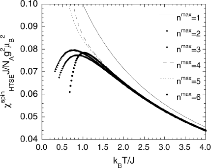
FIG. 10.: High-temperature series expansion predictions of the normalized spin susceptibility $\chi^{\rm spin}_{\rm HTSE}J/N_{\rm A}g^{2}\mu_{\rm B}^{2}$ with $n^{\rm max}=1\mbox{--}6$ versus reduced temperature $k_{\rm B}T/J$ [Eq. (23)] for the antiferromagnetically coupled spins $S=1/2$ in the $B$ sublattice of a normal-spinel compound $A[B_{2}]$O₄.

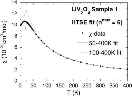
FIG. 11.: Intrinsic susceptibility $\chi$ versus temperature $T$ for LiV₂O₄ sample 1 (filled circles) and fits (curves) by the high-$T$ series expansion (HTSE) prediction to 6th order in $1/T$ for the 50–400 and 100–400 K temperature ranges.

$$\chi(T)=\chi_{0}+\chi^{\rm spin}_{\rm HTSE}(T)~{}~{},$$ (34)

with $\chi^{\rm spin}_{\rm HTSE}(T)$ given by Eq. (23) and the $b_{n}$ coefficients for $S=1/2$ in Eq. (33). The three parameters to be determined are $\chi_{0}$, $g$ and $J/k_{\rm B}$. The fitting parameters for samples 1–7, 4A and 4B using $n^{\rm max}=6$, and for sample 1 also using $n^{\rm max}=2$ and 3, are given in Table IV for the 50–400 and 100-400 K fitting ranges. The fits for these two fitting ranges for sample 1 and $n^{\rm max}=6$ are shown in Fig. 11. Both $g$ and $J/k_{\rm B}$ tend to decrease as the lower limit of the fitting range increases. The HTSE fits for all the samples yielded the ranges $C=N_{\rm A}g^{2}\mu_{\rm B}^{2}/(4k_{\rm B})=0.36\mbox{--}0.48$ cm³ K/(mol V) and $\theta=-20$ to $-42$ K, in agreement with those reported previously (see Table I). $\chi_{0}$ was found to be sensitive to the choice of fitting temperature range. For the 50–400 K range, $\chi_{0}$ was negative for some samples. Recalling the small negative value of the core diamagnetic contribution in Eq. (18) and the larger positive value of the Van Vleck susceptibility in Eqs. (19) and (22), it is unlikely that $\chi_{0}$ [defined below in Eq. (35)] would be negative. Negative values of $\chi_{0}$ occur when the low-$T$ limit of the fitting range is below 100 K, and may therefore be an artifact of the crossover between the local moment behavior at high $T$ and the HF behavior at low $T$.

To eliminate $\chi_{0}$ as a fitting parameter, we also fitted ${\rm d}\chi/{\rm d}T$ by the HTSE prediction for that quantity. The experimental ${\rm d}\chi/{\rm d}T$ was determined from a Padé approximant fit to $\chi(T)$ and is plotted in Fig. 12 for sample 1. These data were fitted by ${\rm d}\chi^{\rm spin}_{\rm HTSE}/{\rm d}T$ obtained from the HTSE prediction Eq. (23) with $n^{\rm max}=6$, where the fitting parameters are now $g$ and $J/k_{\rm B}$. The fits were carried out over the same two $T$ ranges as in Fig. 11; Table V displays the fitting parameters and the fits are plotted in Fig. 12. Both $g$ and $J/k_{\rm B}$ were found to be larger than the corresponding values in Table IV. Of the two fitting ranges, the 100–400 K fit is the best fit inside the respective range, though it shows a large deviation from the data below this range. Using the fitting parameters, the HTSE $\chi^{\rm spin}(T)$ is obtained from Eq. (23). According to Eq. (34), the difference between the experimental $\chi(T)$ and $\chi^{\rm spin}_{\rm HTSE}(T)$, $\delta\chi(T)=\chi(T)-\chi^{\rm spin}_{\rm HTSE}(T)$,

TABLE IV.: Results of high-temperature series expansion calculation fits to the intrinsic magnetic susceptibility data for LiV₂O₄ over the temperature ranges 50–400 K and 100–400 K. The error in the last digit of a quantity is given in parentheses.

Sample	$n^{\rm max}$	50–400 K			100–400 K
No.		$\chi_{0}$	$g$	$J/k_{\rm B}$	$\chi_{0}$	$g$	$J/k_{\rm B}$
		($10^{-4}$ cm3/mol)		(K)	($10^{-4}$ cm3/mol)		(K)
1	2	0.8(4)	2.17(1)	25.8(5)	2.7(3)	2.07(2)	20(1)
1	3	0.7(4)	2.18(2)	26.2(6)	2.6(3)	2.07(2)	20(1)
1	6	0.5(4)	2.19(2)	26.9(7)	2.6(3)	2.07(2)	20(1)
2	6	$-$0.2(5)	2.26(2)	26.7(8)	2.6(3)	2.11(2)	19(1)
3	6	$-$1.3(5)	2.23(2)	27.8(7)	1.4(3)	2.08(2)	20.5(8)
4	6	1.1(6)	2.16(3)	26.4(9)	4.1(5)	1.99(3)	17(2)
4A	6	$-$0.6(8)	2.20(3)	26(1)	2.3(2)	2.05(1)	18.1(6)
4B	6	$-$0.7(5)	2.12(2)	26.2(8)	1.8(5)	1.97(3)	18(2)
5	6	1.2(7)	2.17(3)	25(1)	4.9(7)	1.95(4)	13(2)
6	6	0.8(1)	2.251(6)	26.5(2)	3.3(7)	2.108(4)	18.4(2)
7	6	0.5(3)	2.20(1)	25.8(5)	3.0(1)	2.051(8)	17.5(4)

TABLE V.: Parameters $g$ and $J/k_{\rm B}$ obtained by fitting the temperature $T$ derivative of the experimental intrinsic susceptibility data for LiV₂O₄ samples 1 and 6 by the $T$ derivative of the HTSE spin susceptibility [Eq. (23)] with $n^{\rm max}=6$ for two different temperature ranges of the fit. The $T$-independent susceptibility $\chi_{0}$ was determined by averaging $\delta\chi(T)$, see Fig. 13. The error in the last digit of a quantity is given in parentheses.

	50–400 K			100–400 K
Sample No.	$\chi_{0}$	$g$	$(J/k_{\rm B})$	$\chi_{0}$	$g$	$(J/k_{\rm B})$
	($10^{-4}$ $\frac{{\rm cm}^{3}}{{\rm mol}}$)		(K)	($10^{-4}$ $\frac{{\rm cm}^{3}}{{\rm mol}}$)		(K)
1	$-$1.5(1)	2.275(3)	29.61(7)	2.00(4)	2.103(2)	22.27(8)
6	$-$2.73(5)	2.402(4)	31.61(9)	2.11(1)	2.174(3)	22.1(1)

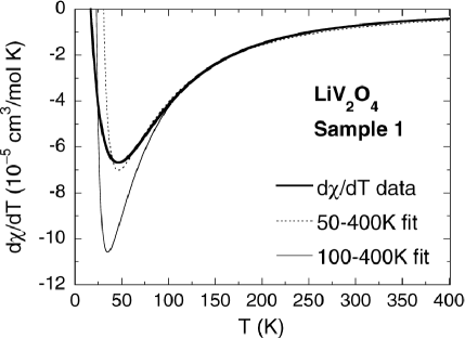
FIG. 12.: Temperature derivative of the experimental intrinsic susceptibility, $d\chi/dT$, for LiV₂O₄ sample 1 (heavy solid curve). Fits by the $T$ derivative of the HTSE prediction $d\chi^{\rm spin}/dT$ in Eq. (23) are also shown for $T$ ranges of 50–400 K (dashed curve) and 100–400 K (light solid curve).

should represent the $T$-independent contribution $\chi_{0}$. $\delta\chi(T)$ is plotted for sample 1 versus $T$ in Fig. 13 for the 50–400 K and 100–400 K fit ranges. Again, the superiority of the 100–400 K fitting range to the other is evident, i.e., $\chi_{0}$ is more nearly constant for this fitting range. $\chi_{0}$ for the 50–400 K fit range is negative within the range. This sign is opposite to that obtained in the

first HTSE fitting results in Table IV. This inconsistency found in the fit using a low $T$ limit below 100 K may again be due to changing physics in the crossover regime, which would invalidate the parameters. By averaging the $\chi_{0}$ values for samples 1 and 6 in the given ranges, we obtained the $T$-independent contribution $\chi_{0}$, as listed in Table V.

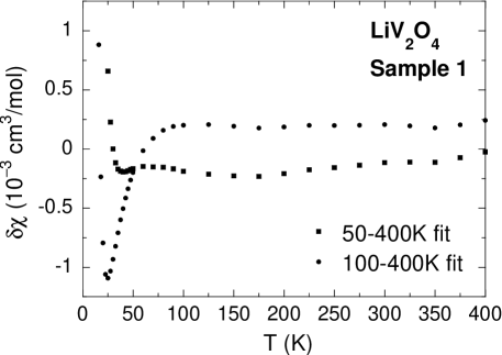
FIG. 13.: The differences between the experimental intrinsic susceptibility $\chi(T)$ of LiV₂O₄ sample 1 and the HTSE prediction $\chi^{\rm spin}$ obtained from the $T$ derivative analysis, $\delta\chi(T)\equiv\chi(T)-\chi^{\rm spin}$, versus temperature $T$ for the fitting $T$ ranges of 50–400 K (open squares) and 100–400 K (filled circles). For a valid fit, these differences should be the $T$-independent susceptibility $\chi_{0}$.

In the itinerant plus localized moment model implicitly assumed in this section, $\chi_{0}$ can be decomposed as

$$\chi_{0}=\chi^{\rm core}+\chi^{\rm VV}+\chi^{\rm Pauli}~{}~{},$$ (35)

where $\chi^{\rm Pauli}$ is the temperature-independent Pauli spin susceptibility of the conduction electrons. Using the results of $\chi^{\rm core}$ [Eq. (18)], $\chi^{\rm VV}$ [Eq. (22)] and $\chi_{0}$ (100–400 K range, Table V), we find

$$\chi^{\rm Pauli}=0.41(10)\times 10^{-4}\,{\rm cm^{3}/mol}~{}~{}({\rm sample~{}1})~{}~{},$$ (37)

$$\chi^{\rm Pauli}=0.52(7)\times 10^{-4}\,{\rm cm^{3}/mol}~{}~{}({\rm sample~{}6})~{}~{}.$$ (38)

These $\chi^{\rm Pauli}$ values are approximately four times smaller than that obtained for LiV₂O₄ by Mahajan et al.[35] They used $\chi^{\rm obs}(T)$ in the $T$ range 100–800 K, combining our $\chi^{\rm obs}(T)$ data to 400 K with those of Hayakawa et al.[14] to 800 K. By fitting these combined data by the expression $\chi^{\rm obs}(T)=\chi_{0}+2C/(T-\theta)$, they obtained $\chi_{0}=5.45\times 10^{-4}$ cm³/mol. As shown above and also discussed in Ref. [35], the value of $\chi_{0}$ is sensitive to the fitting temperature range. For LiTi₂O₄, $\chi^{\rm Pauli}$ $\sim 2\times 10^{-4}$ cm³/mol (Refs. [23, 58]) between 20 and 300 K, which is a few times larger than we find for LiV₂O₄ from the 100–400 K range fits (Table V).

C Crystal Field Model

The ground state of a free ion with one 3$d$ electron is ${}^{2}D_{3/2}$ and has five-fold orbital degeneracy. The point symmetry of a V atom in LiV₂O₄ is trigonal. If we consider the crystalline electric field (CEF) seen by a V atom arising from only the six nearest-neighbor oxygen ions, the CEF due to a perfect oxygen octahedron is cubic ($O_{h}$ symmetry), assuming here point charges for the oxygen ions. In this CEF the degeneracy of the five $d$ orbitals of the vanadium atom is lifted and the orbitals are split by an energy “$10Dq$” into a lower orbital $t_{2g}$ triplet and a higher orbital $e_{g}$ doublet. However, in LiV₂O₄ each V-centered oxygen octahedron is slightly distorted along one of the $<$111$>$ directions [see Fig. 1(b)], as discussed in Sec. III A. This distortion lowers the local symmetry of the V atom to $D_{3d}$ (trigonal) and causes a splitting of the $t_{2g}$ triplet into an $A_{1g}$ singlet and an $E_{g}$ doublet. It is not clear to us which of the $E_{g}$ or $A_{1g}$ levels become the ground state, and how large the splitting between the two levels is. These questions cannot be answered readily without a knowledge of the magnitudes of certain radial integrals,[59] and are not further discussed here.[60] However, this trigonal splitting is typically about an order of magnitude smaller than $10Dq$.[61] In the following, we will examine the predictions for $\chi(T)$ of a $d^{1}$ or $d^{2}$ ion in a cubic CEF and compare with our experimental data for LiV₂O₄.

Kotani[62] calculated the effective magnetic moment $\mu_{\rm eff}\equiv p_{\rm eff}\mu_{\rm B}$ per $d$-atom for a cubic CEF using the Van Vleck formula.[63] The spin-orbit interaction is included, where the coupling constant is $\lambda$. For an isolated atom $\mu_{\rm eff}(T)$ is defined by $\chi(T)\equiv N\mu_{\rm eff}^{2}(T)/(3k_{\rm B}T)$, where $\mu_{\rm eff}$ is in general temperature-dependent and $N$ is the number of magnetic atoms. With spin included, one uses the double group for proper representations of the atomic wavefunctions. Then in this cubic double group with one $d$-electron the six-fold (with spin) degenerate $t_{2g}$ level splits into a quartet $\Gamma_{8}$($t_{2g}$) and a doublet $\Gamma_{7}$($t_{2g}$).[62, 64, 65] The four-fold degenerate $e_{g}$ level does not split and its representation is $\Gamma_{8}$($e_{g}$). For a positive $\lambda$, as is appropriate for a $3d$ atom with a less than half-filled $d$-shell, $\Gamma_{8}$($t_{2g}$) is the ground state, and the first-order Zeeman effect does not split it; this ground state is non-magnetic. Kotani does not include in his calculations of $\mu_{\rm eff}$ the possible coupling of $\Gamma_{8}$($t_{2g}$) and $\Gamma_{8}$($e_{g}$), which have the same symmetry, and assumes that the cubic CEF splitting $10Dq$ is large enough to prevent significant mixing. On the other hand, the cubic double group with two $d$-electrons gives an orbitally nondegenerate, five-fold spin-degenerate, ground state with angular momentum quantum number ${\cal J}=2$ which splits into five non-degenerate levels under a magnetic field. The spin-orbit coupling constant is $\lambda=$ +250 cm^-1 for $d^{1}$ (V⁺⁴) and +105 cm^-1 for $d^{2}$ (V⁺³).[66] The effective moment is defined from the observed molar susceptibility of LiV₂O₄ as $\chi^{\rm obs}(T)=\chi_{0}+2N_{\rm A}[p_{\rm eff}^{\rm obs}(T)]^{2}\mu_{\rm B}^{2}/(3k_{\rm B}T)$, where we take $\chi_{0}=2.00\times 10^{-4}$ cm³/mol given in Table V. Kotani’s results from the Van Vleck equations are[62]

$$p_{\rm eff}^{(1)}=\Biggl{[}\frac{8+(3x-8)e^{-\frac{3}{2}x}}{x(2+e^{-\frac{3}{2}x})}\Biggr{]}^{1/2}~{}~{}$$ (39)

for the $d^{1}$ ion, and

$$p_{\rm eff}^{(2)}=\Biggr{[}\frac{3(\frac{5}{2}x+15+(\frac{x}{2}+9)e^{-x}-24e^{-\frac{3}{2}x})}{x(5+3e^{-x}+e^{-\frac{3}{2}x})}\Biggr{]}^{1/2}~{}~{}$$ (40)

for the $d^{2}$ ion, where $x\equiv\lambda$/$k_{\rm B}T$. Figure 14 shows $p_{\rm eff}^{\rm obs}$, $p_{\rm eff}^{(1)}$ and $p_{\rm eff}^{(2)}$ as a function of $T$. For comparison is also shown $p_{\rm eff}^{(1+2)}$ obtained by assuming that $p_{\rm eff}^{\rm obs}(T)$ arises from an equal mixture of V⁺³ and V⁺⁴ localized moments. None of the three calculated curves agree with the experimental data over the full temperature range. However, in all three calculations $p_{\rm eff}$ increases with $T$, in qualitative agreement with the data, perhaps implying the importance of orbital degeneracy in LiV₂O₄ and/or antiferromagnetic coupling between vanadium spins. The nearly $T$-independent $p_{\rm eff}^{\rm obs}\approx 1.8$ for $T\gtrsim 100$ K is close to the spin-only value $p_{\rm eff}=g\sqrt{S(S+1)}$ with $S=1/2$ and $g\approx 2$, as expected in the absence of orbital degeneracy; however, this result also arises in the theory for the $d^{1}$ ion when $k_{\rm B}T\sim\lambda$, as seen by comparison of the solid curve with the data in Fig. 14 at $\sim 300$ K.

FIG. 14.: Observed effective magnetic moment in $\mu_{\rm B}$, $p_{\rm eff}^{\rm obs}$, versus temperature $T$ of LiV₂O₄ sample 1 (filled diamonds). Also shown as the curves are the predictions $p_{\rm eff}^{(1)}$ for $d^{1}$ ions and $p_{\rm eff}^{(2)}$ for $d^{2}$ ions by Kotani,[62] and $p_{\rm eff}^{(1+2)}$ for an equal mixture of $d^{1}$ and $d^{2}$ ions, in a cubic crystalline electric field, including spin-orbit coupling.

D Spin-1/2 Kondo Model and Coqblin-Schrieffer Model

$\chi^{\rm obs}(T)$ data for $f$-electron HF compounds are often found to be similar to the predictions of the single-ion Kondo model[31, 67, 68, 69, 70] for spin $S=$1/2 or its extention to $S>$ 1/2 in the Coqblin-Shrieffer model.[71, 72] The zero-field impurity susceptibility $\chi_{\rm CS}(T)$ of the Coqblin-Shrieffer model was calculated exactly as a function of temperature by Rajan.[72] His numerical results $\chi_{\rm CS}(T)$ for impurity angular momentum quantum number ${\cal J}=1/2$, …, 7/2 show a Curie-Weiss-like $1/T$ dependence (with logarithmic corrections) for $T\gg T_{\rm K}$, where $T_{\rm K}$ is the Kondo temperature. As $T$ decreases, $\chi_{\rm CS}(T)$ starts to deviate from the $1/T$ dependence, shows a peak (at $T\approx 0.2T_{\rm K}$) only for ${\cal J}\geq 3/2$, and levels off for $T\lesssim 0.2T_{\rm K}$ for all ${\cal J}$.

In the zero temperature limit the molar susceptibility for ${\cal J}=S=1/2$ (which corresponds to the $S=1/2$ Kondo model) is[72]

$$\chi_{\rm CS}(T=0)=\frac{0.102678N_{\rm A}g^{2}\mu^{2}_{\rm B}}{k_{\rm B}T_{\rm K}}~{}~{}.$$ (41)

Setting $g=2$, and using the intrinsic $\chi(T\,\rightarrow\,0)=0.0049$ cm³/(mol V) for LiV₂O₄ sample 1 from Eq. (5), Eq. (41) yields the Kondo temperature

$$T_{\rm K}=32.1\,{\rm K}~{}~{}.$$ (42)

On the other hand, if the $g$-value of 2.10 from Table V (100–400 K range) is employed instead, the Kondo temperature is

$$T_{\rm K}=35.5\,{\rm K}~{}~{}.$$ (43)

The temperature dependence of the impurity susceptibility of the $S=1/2$ Kondo model was obtained using accurate Bethe ansatz calculations by Jerez and Andrei.[73] Their $T\to 0$ value for the coefficient on the right-hand-side of Eq. (41) is 0.1028164, about 0.1% too high compared with the correct prefactor in Eq. (41). We fitted their calculated values for $t=0.00104$ to 102.53 by

$$\frac{4\chi_{\rm CS}k_{\rm B}T}{Ng^{2}\mu^{2}_{\rm B}}=\frac{1+{n_{1}\over t}+{n_{2}\over t^{2}}+{n_{3}\over t^{3}}+{4(0.1028164)n_{5}\over t^{5}}}{1+{d_{1}\over t}+{d_{2}\over t^{2}}+{d_{3}\over t^{3}}+{d_{4}\over t^{4}}+{n_{5}\over t^{6}}}~{}~{},$$ (45)

$$n_{1} = 530.417~{},~{}~{}~{}n_{2}=4697.91~{},~{}~{}~{}n_{3}=1404.18~{},$$ (46)

$$n_{5} = -418.781~{},~{}~{}~{}d_{1}=695.557~{},~{}~{}~{}d_{2}=8605.97~{},$$ (47)

$$d_{3} = 11373.7~{},~{}~{}~{}d_{4}=2937.88~{},$$ (48)

where $t\equiv T/T_{\rm K}$. Equation (45) has the correct form $\chi_{\rm CS}(0)+bt^{2}$ at low $T$ and approaches a Curie law in the high-$T$ limit, as required by the Kondo model. The large $n_{i}$ and $d_{i}$ coefficients arise because $\chi_{\rm CS}(T)$ converges very slowly to the Curie law at high temperatures. The rms deviation of the fit values from the Bethe ansatz calculation values is 0.038%, and the maximum deviation is 0.19% at $t=66.9$. Using the above-stated $g$-values and $T_{\rm K}$ from Eqs. (42) and (43), the $S=1/2$ $\chi_{\rm CS}(T)$ calculations are compared with our $\chi(T)$ data in Fig. 15. Note that in Fig. 15, both the $T$-independent $\chi_{0}$ (Table V) and impurity susceptibilities are already subtracted from $\chi^{\rm obs}$. Although the $T_{\rm K}$ values in Eqs. (42) and (43) are comparable to those obtained from specific heat analyses,[6, 74] the $S=1/2$ Kondo model predictions for $\chi(T)$ with these $T_{\rm K}$ values do not agree with our observed temperature dependence. This failure is partly due to the fact that our $\chi(T)$ data exhibit a weak maximum whereas the $S=1/2$ Kondo model calculation does not.

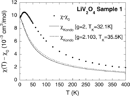
FIG. 15.: Temperature $T$-dependent part of the magnetic susceptibility, $\chi-\chi_{0}$, versus $T$ for LiV₂O₄ sample 1 (filled circles). Also shown as solid and dashed curves are the predictions of the spin $S=1/2$ Kondo model for $(g,\,T_{\rm K})=(2$, 32.1 K) and (2.103, 35.5 K), respectively, where $g$ is the $g$-factor and $T_{\rm K}$ is the Kondo temperature.

As noted above, the Coqblin-Schrieffer model for ${\cal J}\geq 3/2$ does give a peak in $\chi_{\rm CS}(T)$.[72] Defining the ratio

$$r(\%)=100\,\frac{\chi^{\rm peak}_{\rm CS}-\chi_{\rm CS}(0)}{\chi_{\rm CS}(0)}~{}~{},$$ (49)

where $\chi^{\rm peak}_{\rm CS}$ is the value of $\chi_{\rm CS}(T)$ at the peak, the calculations[72] give $r=2$, 7, 11, 17 and 22% for ${\cal J}=3/2$, 2, 5/2, 3 and 7/2, respectively. The observed value is $r=8.2$% in sample 1, which is between the theoretical values for ${\cal J}=2$ and 5/2. Fits of $\chi_{\rm CS}(T)$ to our $\chi(T)$ data of sample 1 for $T=2$–400 K are shown in Fig. 16 and the parameters are

$$\chi_{0} = 2.3(3)\times 10^{-4}\,{\rm cm^{3}/mol}~{},$$ (51)

$$g = 0.790(3)~{},~{}~{}T_{\rm K}=97.8(6)\,{\rm K}~{}~{}({\cal J}=2)~{}~{};$$ (52)

$$\chi_{0} = 6.9(9)\times 10^{-4}\,{\rm cm^{3}/mol}~{},$$ (54)

$$g = 0.591(7)~{},~{}~{}T_{\rm K}=103(2)\,{\rm K}~{}~{}({\cal J}=5/2)~{}~{}.$$ (55)

The ${\cal J}=2$ curve fits our $\chi(T)$ data fairly well. However, the 1.5 $d$-electrons per V ion could not give rise to a ${\cal J}$ value this large; the very small value of $g$ is also considered highly unlikely.

On the basis of the above analysis we conclude that the Coqblin-Schrieffer model for $S>1/2$ and the $S=1/2$ Kondo model cannot explain the intrinsic susceptibility of LiV₂O₄ over any appreciable temperature range.

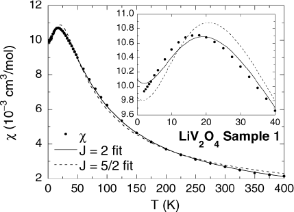
FIG. 16.: Intrinsic magnetic susceptibility $\chi$ of sample 1 versus temperature $T$ and fits by the Coqblin-Schrieffer model prediction for spins ${\cal J}=2$ and 5/2. The inset shows an expanded plot of the data and fits below 40 K.

V Summary and Discussion

In this paper we have described the synthesis and characterization of nine LiV₂O₄ samples. Our magnetically purest samples 1 and 6 clearly showed a broad shallow maximum in the observed magnetic susceptibility $\chi^{\rm obs}(T)$ at $T\approx 16$ K, with small Curie-like upturns below $\sim 5$ K. Field-cooled and zero-field-cooled magnetization measurements with $H=10\mbox{--}100$ G did not reveal any evidence for static spin-glass ordering from 1.8–2 to 50 K in any of the seven samples measured. At $T\gtrsim 50$ K, $\chi^{\rm obs}(T)$ showed local magnetic moment behavior for all samples. In sample 2 which showed a larger Curie-like upturn in $\chi^{\rm obs}(T)$ at low $T$ than in samples 1 and 6, we found that liquid-nitrogen quenching reduced the Curie-like upturn to a large extent, revealing the broad peak in $\chi^{\rm obs}(T)$. However, ice-water quenching and slow-oven cooling enhanced the upturn, and the above successful reduction of the upturn by liquid-nitrogen quenching could not be reproduced. We analyzed low-$T$ isothermal magnetization versus applied magnetic field $M^{\rm obs}(H)$ data, and determined the parameters of the paramagnetic impurities giving rise to the Curie-like upturn in $\chi^{\rm obs}(T)$, assuming that a single type of impurity is present. Using these parameters, the intrinsic susceptibility $\chi(T)$ was obtained and found to be essentially the same in all samples but one (4A). Surprisingly, the spin $S_{\rm imp}$ of the paramagnetic impurities was found to be large, $S_{\rm imp}=3/2$ to 4 depending on the sample, suggesting the presence of variable amounts of ferromagnetically coupled vanadium spin defect clusters of variable size in the samples.

We tested the localized magnetic moment picture for $\chi(T)$ at $T\gtrsim 50$ K using the HTSE prediction for the spin susceptibility of the $S=1/2$ vanadium sublattice of the spinel structure, which yielded $C$ and $\theta$ values similar to those reported in the past for LiV₂O₄. Using the values of the Van Vleck susceptibility obtained from $K$-$\chi$ analyses, the Pauli susceptibility contribution to the temperature-independent susceptibility $\chi_{0}$ was derived and found to be small, comparable to that of LiTi₂O₄. The Van Vleck formulas for the paramagnetic susceptibility of isolated V⁺³ or V⁺⁴ ions or an equal mixture, assuming that each V ion is in a cubic CEF, failed to describe the $T$ dependence of the observed effective magnetic moment. For the high-$T$ “localized moment” region, the observed effective moment is in agreement with the spin-only value expected for $g\simeq 2$.

Our attempts to describe the low-$T$ susceptibility data in terms of the single-ion Kondo ($S=1/2$) and Coqblin-Schrieffer (${\cal J}$ or $S>1/2$) models for isolated magnetic impurities in metals were unsuccessful. These models predict that the electronic specific heat coefficient $\gamma(T)$ and the susceptibility $\chi(T)$ both show maxima for ${\cal J}\geq 3/2$.[72] LiV₂O₄ clearly shows a peak in $\chi(T)$ at $T\approx 16$ K, but there is no peak in $\gamma(T)$ down to 1.2 K.[6, 74] Thus, these theories cannot self-consistently explain the results of both measurements, suggesting that there is some other mechanism responsible for the heavy-fermion behavior and/or that the single-ion picture is inappropriate. It is however intriguing that the experimental Wilson ratio $R_{\rm W}\approx 1.7$ at 1 K (Ref. [6]) is close to that ($R_{\rm W}=2$) predicted for the $S=1/2$ Kondo model.

In conventional $f$-electron heavy fermion compounds, local $f$-electron orbitals and conduction electron states in non-$f$ bands hybridize only weakly, resulting in a many-body scattering resonance of the quasiparticles near the Fermi energy $E_{\rm F}$, a large density of quasiparticle states ${\cal D}(E_{\rm F})$, and hence a large quasiparticle effective mass, electronic specific heat coefficient and magnetic spin susceptibility at low $T$. Screening of $S=1/2$ local moments by conduction electron spins leads to a nonmagnetic ground state and a saturating spin susceptibility as $T\rightarrow 0$. In Sec. IV, we tested several models for $\chi(T)$ which assume the presence of local magnetic moments in LiV₂O₄ which interact weakly with the conduction electrons. However, in these models as applied to LiV₂O₄, the itinerant and “localized” electrons must both occupy $t_{2g}$ orbitals (or bands derived from these orbitals), rather than orbitals of more distinct character. One can imagine a scenario in which the HF behaviors of LiV₂O₄ at low $T$ arise in a way similar to that of the $f$-electron HF compounds, if the following conditions are fulfilled: (i) the trigonal component of the CEF causes the $A_{1g}$ orbital singlet to lie below the $E_{g}$ orbital doublet; (ii) one of the 1.5 $d$-electrons/V is localized in the ground $A_{1g}$ orbital due to electron-electron correlations;[75] (iii) the remaining 0.5 $d$-electron/V occupies the $E_{g}$ doublet and is responsible for the metallic character; and (iv) the band(s) formed from the $E_{g}$ orbitals hybridize only weakly with the $A_{1g}$ orbital on each V ion. This scenario involves a kind of orbital ordering; a more general discussion of orbital ordering effects is given below.

The geometric frustration for antiferromagnetic ordering inherent in the V sublattice of LiV₂O₄ may be important to the mechanism for the observed HF behaviors of this compound at low $T$. Such frustration inhibits long-range magnetic ordering and enhances quantum spin fluctuations and (short-range) dynamical spin ordering.[16, 17, 76] These effects have been verified to occur in the C15 fcc Laves phase intermetallic compound (Y_0.97Sc_0.03)Mn₂, in which the Y and Sc atoms are nonmagnetic and the Mn atom substructure is identical with that of V in LiV₂O₄. In (Y_0.97Sc_0.03)Mn₂, Shiga et al. discovered quantum magnetic moment fluctuations with a large amplitude ($\mu_{\rm rms}=1.3\,\mu_{\rm B}$/Mn at 8 K) in their polarized neutron scattering study.[77] They also observed a thermally-induced contribution, with $\mu_{\rm rms}=1.6\,\mu_{\rm B}$/Mn at 330 K. Further, Ballou et al.[29] inferred from their inelastic neutron scattering experiments the presence of “short-lived 4-site collective spin singlets,” thereby suggesting the possibility of a quantum spin-liquid ground state. A recent theoretical study by Canals and Lacroix[76] by perturbative expansions and exact diagonalization of small clusters of a $S=1/2$ (frustrated) pyrochlore antiferromagnet[78] found a spin-liquid ground state and an AF spin correlation length of less than one interatomic distance at $T=0$. Hence, it is of great interest to carry out neutron scattering measurements on LiV₂O₄ to test for similarities and differences in the spin excitation properties to those of (Y_0.97Sc_0.03)Mn₂.

(Y_0.97Sc_0.03)Mn₂ has some similarities in properties to those of LiV₂O₄. No magnetic long-range ordering was observed above 1.4 K (Refs. [29, 77]) and 0.02 K,[6] respectively. Similar to LiV₂O₄, (Y_0.97Sc_0.03)Mn₂ shows a large electronic specific heat coefficient $\gamma(0)\approx 160\mbox{--}200$ mJ/mol K².[29, 79] However, the $T$ dependences of the susceptibility[80] and $\gamma$ (Ref. [79]) are very different from those seen in LiV₂O₄ and in the heaviest $f$-electron heavy fermion compounds. $\chi^{\rm obs}(T)$ does not show a Curie-Weiss-like behavior at high $T$, but rather increases with increasing $T$.[80] $\gamma(T)$ is nearly independent of $T$ up to at least 6.5 K.[79] Replacing a small amount of Mn with Al, Shiga et al. found spin-glass ordering in (Y_0.95Sc_0.05)(Mn_1-xAl_x)₂ with $x\geq 0.05$.[81] The susceptibility for $x=0.15$ shows a Curie-Weiss-like behavior above $\sim 50$ K. The partial removal of the geometric frustration upon substitution of Al for Mn might be anologous to that in our sample 3 in which structural defects evidently ameliorate the frustrated V-V interactions, leading to spin-glass ordering below $\sim 0.8$ K.[6]

The magnetic properties of materials can be greatly influenced when the ground state has orbital degeneracy in a high-symmetry structure. Such degenerate ground state orbitals can become energetically unstable upon cooling. The crystal structure is then deformed to a lower symmetry to achieve a lower-energy, non-orbitally-degenerate ground state (Jahn-Teller theorem).[82] This kind of static orbital ordering accompanied by a structural distortion is called the cooperative Jahn-Teller effect.[82] The driving force for this effect is the competition between the CEF and the lattice energies. Orbital ordering may also be caused by spin exchange interactions in a magnetic system with an orbitally-degenerate ground state.[82, 83] The orbital (and charge) degrees of freedom may couple with those of the spins in such a way that certain occupied orbitals become energetically favorable, and consequently the degeneracy is lifted. As a result, the exchange interaction becomes spatially anisotropic. For example, Pen et al.[83] showed that the degenerate ground states in the geometrically frustrated V triangular lattice Heisenberg antiferromagnet LiVO₂ can be lifted by a certain static orbital ordering. X-ray and neutron diffraction measurements detected no structural distortions or phase transitions in LiV₂O₄.[6, 39] However, the presence of orbital degeneracy or near-degeneracy suggests that dynamical orbital-charge-spin correlations may be important to the physical properties of LiV₂O₄. It is not yet known theoretically whether such dynamical correlations can lead to a HF ground state and this scenario deserves further study.

Thus far we and collaborators have experimentally demonstrated heavy fermion behaviors of LiV₂O₄ characteristic of the heaviest-mass $f$-electron HF systems from magnetization,[6] specific heat,[6, 74] nuclear magnetic resonance,[6, 35] thermal expansion,[39, 74] and muon spin relaxation[6] measurements. Our magnetization study reported in this paper was done with high-purity polycrystalline samples from which we have determined the low temperature intrinsic susceptibility. Nevertheless, high-quality single crystals are desirable to further clarify the physical properties. In particular, it is crucial to measure the low-$T$ resistivity, the carrier concentration and the Fermi surface. In addition, when large crystals become available, inelastic neutron scattering experiments on them will be vital for a deeper understanding of this $d$-electron heavy fermion compound.

On the theoretical side, new physics may be necessary to explain the heavy fermion behaviors we observe in LiV₂O₄. We speculate that the geometric frustration for antiferromagnetic ordering and/or coupled dynamical orbital-charge-spin correlations may contribute to a new mechanism leading to a heavy fermion ground state. A successful theoretical framework must in any case self-consistently explain the radically different properties of LiV₂O₄ and the isostructural superconductor LiTi₂O₄.

- [1] K. Andres, J. E. Graebner, and H. R. Ott, Phy. Rev. Lett. 35, 1779 (1975).
- [2] J. G. Bednorz and K. A. Müller, Z. Phys. B 64, 189 (1986).
- [3] For reviews, see, e.g., J. M. Lawrence, P. S. Riseborough, and R. D. Parks, Rep. Prog. Phys. 44, 1 (1981); G. R. Stewart, Rev. Mod. Phys. 56, 755 (1984); N. B. Brandt and V. V. Moshchalkov, Adv. Phys. 33, 373 (1984); P. Schlottmann, Phys. Rep. 181, 1 (1989); N. Grewe and F. Steglich, Ch. 97 in Handbook on the Physics and Chemistry of Rare Earths, Vol. 14, eds. K. A. Gschneidner, Jr. and L. Eyring (Elsevier, Amsterdam, 1991), pp. 343–474; G. Aeppli and Z. Fisk, Comments Cond. Mat. Phys. 16, 155 (1992); M. Loewenhaupt and K. H. Fischer, Ch. 105 in Handbook on the Physics and Chemistry of Rare Earths, Vol. 16, eds. K. A. Gschneidner, Jr. and L. Eyring (Elsevier, Amsterdam, 1993), pp. 1–105; A. C. Hewson, The Kondo Problem to Heavy Fermions (Cambridge University Press, Cambridge, 1993).
- [4] M. B. Maple, C. L. Seaman, D. A. Gajewski, Y. Dalichaouch, V. B. Barbetta, M. C. de Andrade, H. A. Mook, H. G. Lukefahr, O. O. Bernal, and D. E. MacLaughlin, J. Low Temp. Phys. 95, 225 (1994).
- [5] U. Zülicke and A. J. Millis, Phys. Rev. B 51, 8996 (1995), and references therein.
- [6] S. Kondo, D. C. Johnston, C. A. Swenson, F. Borsa, A. V. Mahajan, L. L. Miller, T. Gu, A. I. Goldman, M. B. Maple, D. A. Gajewski, E. J. Freeman, N. R. Dilley, R. P. Dickey, J. Merrin, K. Kojima, G. M. Luke, Y. J. Uemura, O. Chmaissem, and J. D. Jorgensen, Phys. Rev. Lett. 78, 3729 (1997).
- [7] B. Reuter and J. Jaskowsky, Angew. Chem. 72, 209 (1960).
- [8] International Tables for Crystallography (Kluwer Academic, Dordrecht, 1987), Vol. A.
- [9] D. B. Rogers, J. L. Gillson, and T. E. Gier, Solid State Commun. 5, 263 (1967).
- [10] H. Kessler and M. J. Sienko, J. Chem. Phys. 55, 5414 (1971).
- [11] Y. Nakajima, Y. Amamiya, K. Ohnishi, I. Terasaki, A. Maeda, and K. Uchinokura, Physica C 185–189, 719 (1991).
- [12] B. L. Chamberland and T. A. Hewston, Solid State Commun. 58, 693 (1986).
- [13] F. Takagi, K. Kawakami, I. Maekawa, Y. Sakai, and N. Tsuda, J. Phys. Soc. Jpn. 56, 444 (1987).
- [14] T. Hayakawa, D. Shimada, and N. Tsuda, J. Phys. Soc. Jpn. 58, 2867 (1989).
- [15] D. C. Johnston, T. Ami, F. Borsa, M. K. Crawford, J. A. Fernandez-Baca, K. H. Kim, R. L. Harlow, A. V. Mahajan, L. L. Miller, M. A. Subramanian, D. R. Torgeson, and Z. R. Wang, Springer Ser. Solid State Sci. 119, 241 (1995).
- [16] P. W. Anderson, Phys. Rev. 102, 1008 (1956).
- [17] J. Villain, R. Bidaux, J. P. Carton, and R. Conte, J. Phys. (Paris) 41, 1263 (1980).
- [18] B. Reuter and J. Jaskowsky, Ber. Bunsenges. Phys. Chem. 70, 189 (1966).
- [19] D. B. Rogers, J. B. Goodenough, and A. Wold, J. Appl. Phys. 35, 1069 (1964).
- [20] E. Pollert, Czech. J. Phys. B 23, 468 (1973); Krist. Tech. 8, 859 (1973).
- [21] D. Arndt, K. Müller, B. Reuter, and E. Riedel, J. Solid State Chem. 10, 270 (1974).
- [22] Y. Ueda, N. Fujiwara, and H. Yasuoka, J. Phys. Soc. Jpn. 66, 778 (1997).
- [23] D. C. Johnston, J. Low Temp. Phys. 255, 145 (1976).
- [24] A. Fujimori, K. Kawakami, and N. Tsuda, Phys. Rev. B 38, 7889 (1988).
- [25] M. Abbate, F. M. de Groot, J. C. Fuggle, A. Fujimori, Y. Tokura, Y. Fujishima, O. Strebel, M. Domke, G. Kaindl, J. van Elp, B. T. Thole, G. A. Sawatzky, M. Sacchi, and N. Tsuda, Phys. Rev. B 44, 5419 (1991).
- [26] S. Satpathy and R. M. Martin, Phys. Rev. B 36, 7269 (1987).
- [27] S. Massida, J. Yu, and A. J. Freeman, Phy. Rev. B 38, 11 352 (1988).
- [28] M. Onoda, H. Imai, Y. Amako, and H. Nagasawa, Phys. Rev. B 56, 3760 (1997).
- [29] R. Ballou, E. Lelièvre-Berna, and B. Fåk, Phys. Rev. Lett. 76, 2125 (1996).
- [30] S. A. Carter, T. F. Rosenbaum, P. Metcalf, J. M. Honig, and J. Spalek, Phys. Rev. B 48, 16 841 (1993).
- [31] K. G. Wilson, Rev. Mod. Phys. 47, 773 (1975).
- [32] Y. Amako, T. Naka, M. Onoda, H. Nagasawa, and T. Erata, J. Phys. Soc. Jpn. 59, 2241 (1990).
- [33] N. Fujiwara, Y. Ueda, and H. Yasuoka, Physica B 237–238, 59 (1997).
- [34] N. Fujiwara, H. Yasuoka, and Y. Ueda, Phy. Rev. B 57, 3539 (1998).
- [35] A. V. Mahajan, R. Sala, E. Lee, F. Borsa, S. Kondo, and D. C. Johnston, Phys. Rev. B 57, 3539 (1998).
- [36] Y. Ueda (private communication).
- [37] F. Izumi, in The Rietveld Method, edited by R. A. Young (Oxford University Press, Oxford, 1993), Ch. 13.
- [38] F. Izumi (private communication).
- [39] O. Chmaissem, J. D. Jorgensen, S. Kondo, and D. C. Johnston, Phys. Rev. Lett. 79, 4886 (1997).
- [40] G. Blasse, Philips Res. Reports Suppl. 3 (1964).
- [41] M. Dalton, I. Gameson, A. R. Armstrong, and P. P. Edwards, Physica C 221, 149 (1994).
- [42] A. Reisman and J. Mineo, J. Phys. Chem. 66, 1184 (1962).
- [43] Y. Ueda, J. Kikuchi, and H. Yasuoka, J. Magn. Magn. Mater. 147, 195 (1995).
- [44] S. Nagata, P. H. Keesom, and S. P. Faile, Phy. Rev. B 20, 2886 (1979).
- [45] A. H. Lacerda, et al. (unpublished).
- [46] Yu. M. Belyakov, V. A. Perelyaev, A. K. Chirkov, and G. P. Shveikin, Russ. J. Inorg. Chem. 18, 1789 (1973).
- [47] T. Palanisamy, J. Gopalakrishnan, and M. V. C. Sastri, J. Solid State Chem. 9, 273 (1974).
- [48] J. Gendell, R. M. Cotts, and M. J. Sienko, J. Chem. Phys. 37, 220 (1962).
- [49] For reviews, see, J. A. Mydosh, Spin Glasses: An Experimental Introduction, (Taylor and Francis, London, 1993).
- [50] R. M. White, Quantum Theory of Solids, 2nd Edition (Springer Verlag, Berlin, 1983) [From Eq. (3.97) on p. 96, , where is the band mass. So is expected to be negligibly small for -electron system whose band width is normally narrow (i.e. is large).]
- [51] M. Takigawa, E. T. Ahrens, and Y. Ueda, Phys. Rev. Lett. 76, 283 (1996).
- [52] J. P. Pouget, P. Lederer, D. S. Schreiber, H. Launois, D. Wohlleben, A. Casalot, and G. Villeneuve, J. Phys. Chem. Solids 33, 1961 (1972).
- [53] P. W. Selwood, Magnetochemistry, 2nd Edition (Interscience, New York, 1956), p. 78.
- [54] E. D. Jones, Phys. Rev. 137, A978 (1965).
- [55] J. Kikuchi, H. Yasuoka, Y. Kokubo, Y. Ueda, and T. Ohtani, J. Phys. Soc. Jpn. 65, 2655 (1996).
- [56] G. S. Rushbrooke and P. J. Wood, Mol. Phys. 1, 257 (1958).
- [57] For a review, see G. S. Rushbrooke, G. A. Baker, and P. J. Wood, in Phase Transitions and Critical Phenomena, Vol. 3, edited by C. Domb and M. S. Green (Academic Press, London, 1974), Ch. 5.
- [58] J. M. Heintz, M. Drillon, R. Kuentzler, Y. Dossmann, J. P. Kappler, O. Durmeyer, and F. Gautier, Z. Phys. B 76, 303 (1989).
- [59] M. Gerloch, J. Lewis, G. G. Phillips, and P. N. Quested, J. Chem. Soc. (A) 1941 (1970).
- [60] S. Kondo (unpublished).
- [61] S. Krupička and P. Novák, in Ferromagnetic Materials, Vol. 3, edited by E. P. Wohlfarth (North-Holland, New York, 1982), Ch. 4.
- [62] M. Kotani, J. Phys. Soc. Jpn. 4, 293 (1949).
- [63] J. H. Van Vleck, Theory of Electric and Magnetic Susceptibilities (Oxford University Press, London, 1932).
- [64] C. J. Ballhausen, Introduction to Ligand Field Theory (McGraw- Hill, New York, 1962), p. 68.
- [65] T. M. Dunn, Some Aspects of Crystal Field Theory (Harper & Row, New York, 1965), Ch. 3.
- [66] T. M. Dunn, Trans. Faraday Soc. 57, 1441 (1961).
- [67] H. R. Krishna-murthy, J. W. Wilkins, and K. G. Wilson, Phys. Rev. B 21, 1003 (1980).
- [68] H. R. Krishna-murthy, J. W. Wilkins, and K. G. Wilson, Phys. Rev. B 21, 1044 (1980).
- [69] V. T. Rajan, J. H. Lowenstein, and N. Andrei, Phys. Rev. Lett. 49, 497 (1982).
- [70] A. M. Tsvelick and P. B. Wiegmann, Adv. Phys. 32, 453 (1983).
- [71] B. Coqblin and J. R. Schrieffer, Phys. Rev. 185, 847 (1969).
- [72] V. T. Rajan, Phys. Rev. Lett. 51, 308 (1983).
- [73] A. Jerez and N. Andrei (unpublished).
- [74] D. C. Johnston, C. A. Swenson, and S. Kondo (unpublished).
- [75] J. B. Goodenough (private communication).
- [76] B. Canals and C. Lacroix, Phys. Rev. Lett. 80, 2933 (1998).
- [77] M. Shiga, H. Wada, Y. Nakamura, J. Deportes, B. Ouladdiaf, and K. R. A. Ziebeck, J. Phys. Soc. Jpn. 57, 3141 (1988), and references therein.
- [78] B. D. Gaulin, J. N. Reimers, T. E. Mason, J. E. Greedan, and Z. Tun, Phys. Rev. Lett. 69, 3244 (1992).
- [79] H. Wada, M. Shiga, and Y. Nakamura, Physica B 161, 197 (1989).
- [80] H. Nakamura, H. Wada, K. Yoshimura, M. Shiga, Y. Nakamura, J. Sakurai, and Y. Komura, J. Phys. F 18, 981 (1988).
- [81] M. Shiga, K. Fujisawa, and H. Wada, J. Phys. Soc. Jpn. 62, 1329 (1993).
- [82] K. I. Kugel’ and D. I. Khomskiĭ, Sov. Phys. JETP 37, 725 (1973).
- [83] H. F. Pen, J. van den Brink, D. I. Khomskii, and G. A. Sawatzky, Phys. Rev. Lett. 78, 1323 (1997).