Leipzig Preprint NTZ 29/1998

Annalen
der Physik
© Johann Ambrosius Barth 1998
Energy barriers of spin glasses from multi-overlap simulations
Wolfhard Janke^1,2, Bernd A. Berg^3,4 and Alain Billoire^5
1Institut für Theoretische Physik, Universität Leipzig, D-04109 Leipzig, Germany
²Institut für Physik, Johannes Gutenberg-Universität, D-55099 Mainz, Germany
³Department of Physics, The Florida State University, Tallahassee, FL 32306, USA
⁴Supercomputer Computations Research Institute, Tallahassee, FL 32306, USA
⁵Service de Physique Théorique de Saclay, F-91191 Gif-sur-Yvette, France
wolfhard.janke@itp.uni-leipzig.de, berg@hep.fsu.edu, billoir@spht.saclay.cea.fr
Received 12 October 1998, revised version 12 October 1998, accepted 12 October 1998
Abstract. We report large-scale simulations of the three-dimensional Edwards-Anderson Ising spin glass system using the recently introduced multi-overlap Monte Carlo algorithm. In this approach the temperature is fixed and two replica are coupled through a weight factor such that a broad distribution of the Parisi overlap parameter $q$ is achieved. Canonical expectation values for the entire $q$-range (multi-overlap) follow by reweighting. We present an analysis of the performance of the algorithm and in particular discuss results on spin glass free-energy barriers which are hard to obtain with conventional algorithms. In addition we discuss the non-trivial scaling behavior of the canonical $q$-distributions in the broken phase.
Keywords: Ising spin glass; Multi-overlap simulations; Energy barriers; Finite-size scaling

1 Introduction

The intuitive picture for spin glasses and other systems with conflicting constraints, for reviews see [1], is that there exists a large number of degenerate thermodynamic states with the same macroscopic properties but with different microscopic configurations. These states are separated by free-energy barriers in phase space, caused by disorder and frustration. Experimentally this is supported by long characteristic times found in phenomena like the measurement of the remanent magnetization in typical spin glasses such as, e.g., $({\rm Fe}_{0.15}{\rm Ni}_{0.85})_{75}{\rm P}_{16}{\rm B}_{6}{\rm Al}_{3}$ [2]. However, one difficulty of the theory of spin glasses is to give a precise meaning to this classification: No explicit order parameter exists which allows to exhibit the barriers. The way out of this problem appears to use an implicit parametrization, the Parisi overlap parameter $q$, which allows to visualize at least some of them [1]. Calculations of the thus encountered barriers in $q$ are of major interest. For instance, it is unclear whether the degenerate thermodynamic states are separated by infinite barriers or whether this is just an artifact of mean-field theory.

Before performing numerical calculations of these barriers, one of the questions which ought to be addressed is “What are suitable weight factors for the problem?” The weight factor of canonical Monte Carlo (MC) simulations is $\exp(-\beta E)$, where $E$ is the energy of the configuration to be updated and $\beta$ is the inverse temperature in natural units. The Metropolis and other MC methods generate canonical configurations through a Markov process. However, by their very definition the rare-event states associated with the free-energy barriers are suppressed in such an ensemble. Now, it became widely recognized in recent years that MC simulations with a-priori unknown weight factors, like for instance the inverse spectral density $1/n(E)$, are also feasible and deserve to be considered, for reviews see [3]. Along such lines progress has been made by exploring [4–7] innovative weighting methods for the spin glass problem.

The main idea of the studies [4–7] is to avoid getting stuck in metastable low-energy states by using a Markov process which samples the ordered as well as the disordered regions of configuration space in one run. Refreshing the system in the disordered phase clearly benefits the simulations, but the performance has remained below early expectation. One reason appears to be that the direct (i.e. ignoring the dynamics of the system) barrier weights are not affected, such that the simulation slows down due to the tree-like structure of the low-energy spin glass states, see Ref. [8] for a detailed discussion.

In Ref. [9] two of the authors introduced a method which focuses directly on enhancing the probability for sampling the barrier regions in the Parisi overlap parameter. Relying on this method, we have meanwhile performed large-scale simulations of the three-dimensional Edwards-Anderson Ising spin glass. First results from this novel investigation are reported in the following. The next section briefly introduces the spin glass model and is followed by an introduction to the method of [9] in section 3. Technical details of the computer simulation are described in section 4 and some of the obtained physical results are summarized in section 5, followed by conclusions in the final section 6.

2 Model

We focus on the three-dimensional ($3d$) Edwards-Anderson Ising (EAI) spin glass on a simple cubic lattice of size $N=L^{3}$ with periodic boundary conditions. It is widely considered to be the simplest model to exhibit realistic spin glass behavior and has been the testing ground of Refs. [4–7]. The energy is given by

$$E=-\sum_{\langle ik\rangle}J_{ik}\,s_{i}s_{k}\qquad,$$ (1)

where the sum is over nearest-neighbour sites and the Ising spins $s_{i}$ and $s_{k}$ take values $\pm 1$. The exchange coupling constants $J_{ik}$ are quenched random variables which are chosen to be $\pm 1$ with equal probability. Each fixed assignment of the exchange coupling constants $J_{ik}$ defines a realization of the system, and all physical results refer to an average over many such realizations. Early MC simulations of the $3d$ EAI model located the freezing temperature at $\beta_{c}\approx 0.9$. For a concise review, see Ref. [7]. Recent, very high-statistics canonical simulations [10] estimate $\beta_{c}=0.901\pm~{}0.034$, and were interpreted [7] to improve the evidence in support of a second-order phase transition at $\beta_{c}$.

The Parisi overlap parameter is defined as [1]

$$q={1\over N}\sum_{i=1}^{N}s_{i}^{1}s_{i}^{2}\qquad,$$ (2)

where the spins $s^{1}_{i}=\pm 1$ and $s^{2}_{i}=\pm 1$ correspond to two independent copies (replica) of the same realization (defined by its couplings $J_{ik}$), each with its own time evolution in the MC simulation (realized by different random numbers).

3 Multi-overlap algorithm

The method of Ref. [9] simulates two replica of the same realization in one computer run. In another context this has before been done in [5]. Our basic observation, closely related to multicanonical methods [3, 4], is that one does still control canonical expectation values at temperature $\beta^{-1}$ when one simulates with a weight function

$$w(q)=\exp\left[\beta\sum_{\langle ik\rangle}J_{ik}(s^{1}_{i}s^{1}_{k}+s^{2}_{i}s^{2}_{k})+S(q)\right]\qquad.$$ (3)

Of particular interest is to determine $S(q)$ recursively such that the $q$-distribution becomes uniform in $q$ (“multi-overlap”), and the interpretation of $S(q)$ being the microcanonical entropy of the Parisi order parameter. Hence, although an explicit order parameter does not exist, an approach very similar to the multimagnetical [11] (which is an highly efficient way to sample interface barriers for ferromagnets) exists herewith.

As a measure of the performance of the algorithm we recorded the average number of sweeps that are necessary to perform tunneling events of the form

$$(q=0)\to(q=\pm 1)~{}~{}{\rm and\ back}.$$

In the following we refer to this quantity as autocorrelation time.

4 Simulation

The multi-overlap algorithm is thus particularly designed for simulations of the interesting region below the freezing temperature where $P_{i}(q)$, the canonical probability density of $q$ for realization $i$ (additional dependence on lattice size and temperature is implicit), exhibits a rather complicated behavior. The shape of $P_{i}(q)$ ranges from a simple double-peak structure to involved structures of several minima and maxima. A few examples encountered in the simulations of the $12^{3}$ system are shown in Fig. 1. This is the situation which is notoriously difficult to study with standard algorithms. In our EAI study we therefore focussed on simulations at $\beta=1>\beta_{c}\approx 0.9$. We investigated lattices of size $N=L^{3}$ with $L=4$, 6, 8, and 12, using T3E parallel computers in Grenoble, Berlin, and Jülich. We simulated 4096 different realizations for the smaller systems up to $L=8$, and 512 for $L=12$, using the Marsaglia random number generator RANMAR [12] for drawing the $J_{ik}$. As a check we also simulated a second set of 4096 realizations for $L=4$, 6, and 8, where the $J_{ik}$ were generated with a more elaborate version of RANMAR: RANLUX [13] with luxury level 4. In the simulations themselves we always employed the RANMAR generator due to CPU time considerations.

Fig. 1: Zoo of probability densities $P_{i}(q)$ for the $12^{3}$ system at $\beta=1$. The subscript $i=1,\dots,512$ labels the different realizations.

For each realization the simulation consisted of three steps:

1. Construction of the weight function (3). Here we employed an improved variant of the accumulative iteration scheme discussed in Ref. [14]. Details will be published elsewhere. The iteration was stopped after at least 10 tunnelings (between $4-20$ for $L=12$) occurred.

2. Equilibration run. This run was to equilibrate the system for given fixed weight factors.

3. Production run. Each production run of data taking was concluded after at least 20 tunneling events were recorded. To allow for easy (standard) reweighting in temperature we stored besides the Parisi overlap parameter also the energies and magnetizations of the two replica in a time-series file. Since the corresponding autocorrelation times $\tau$ vary significantly from realization to realization we used an adaptive data compression routine to make sure that the spacing between measurements was always proportional to $\tau$. Using this adaptive scheme we recorded for each realization 65536 measurements.

Let us conclude this section with a few remarks on the performance of the new algorithm. Fitting the estimates of the mean autocorrelation time $[\tau]_{\rm av}$ to the form $\ln([\tau]_{\rm av})=a+z\,\ln(N)$ gives $z=2.42\pm 0.03$. As will be discussed below, the implied improvement with respect to barrier calculations is huge. Nevertheless the slowing down is quite off from the theoretical optimum, which is $z=1$ for multicanonical simulations [3]. One reason seems to be that we want the $q$-distribution to be uniform in the whole admissible interval $q\in[-1,+1]$, including the region of $|q|\approx 1$ that is strongly correlated with ground states and hence difficult to reach by local updates, see for instance [8]. Being content with a smaller region (like the region between the two outmost maxima of $P_{i}(q)$) is expected to give further improvements of the tunneling performance. By also monitoring the encountered minimum, maximum and median tunneling times we observed that the mean values are systematically larger than the median, what means that the tunneling distribution has a rather long tail towards large tunneling times. On the other hand, the effect is not severely hindering our multi-overlap simulations: For the lattice sizes $L=4$ to 8 the worst behaved realization took never more than 1% of the entire computer time. Indicating a remarkable increase of complexity, this amount was about 12% for $L=12$.

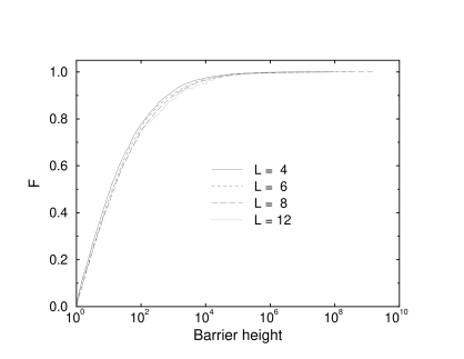
Fig. 2: Integrated probability density $F$ of canonical tunneling barrier heights at $\beta=1$.

5 Results

The data created in this way allows us to calculate a number of physically interesting quantities. Let us first concentrate on the canonical potential barriers in $q$ which were in Ref. [9] defined as

$$B_{i}=\prod_{q=-1}^{-\,\triangle q}\max\left[1,P_{i}(q)/P_{i}(q+\triangle q)\right]\qquad,$$ (4)

where $\triangle q$ is the step-size in $q$. For the double-peak situations of first-order phase transitions [11] Eq. (4) simplifies to $B_{i}=P_{i}^{\max}/P_{i}^{\min}$, where $P_{i}^{\max}$ is the absolute maximum and $P_{i}^{\min}$ is the absolute minimum (for ferromagnets at $q=0$) of the probability density $P_{i}(q)$. Our definition generalizes to the situation where several minima and maxima occur due to disorder and frustration. When evaluating (4) from numerical data for $P_{i}(q)$ some care is needed to avoid contributions from statistical fluctuations of $P_{i}(q)$.

Graphically, our values for the $B_{i}$ are presented in Fig. 2. It comes as a surprise that the finite-size dependence of the distributions is very weak. To study this issue further, we have compiled in Table 1 for each lattice size the following informations about our potential barrier results: largest and second largest values $B_{\rm max}$ and $B_{2}$, median values $B_{\rm med}$ and mean values $[B]_{\rm av}$ with their statistical error bars. From this table it becomes obvious, why this investigation could not be performed using canonical methods to which in this context also multicanonical simulations and enlarged ensembles belong, as their weights for those barriers are still canonical. For these methods the slowing down is proportional to the average barrier height $[B]_{\rm av}$, which is already large for $L=4$, about 17 thousand, and increases to about 250 thousand for $L=8$. The subsequent decrease to about 150 thousand for $L=12$ has to be attributed to the smaller number of realizations in this case: Comparison of the extrem values makes only sense when the numbers of realizations match. On $L=4$ and $L=6$ systems we have performed a number of (very long) canonical simulations to estimate the proportionality constant between barrier height and improvement due to our multi-$q$ simulations. Using these result, we estimate that with our computer program a canonical MC calculation of the worst $L=12$ barrier alone, the one reported in Table 1, would take about 1000 years on a 500 MHz Alpha processor.

Table 1: Canonical potential barriers: maximum (and its contribution to the mean in %), second largest value, the median and its jackknife error bar, the mean and its (standard) error bar.

$L$	$B_{\max}$	$B_{2}$	$B_{\rm med}$	$[B]_{\rm av}$
4	8.76E07 (62%)	6.01E06	$11.05\pm 0.24$	$(1.72\pm 1.08)$E04
6	3.73E08 (41%)	3.63E08	$12.83\pm 0.45$	$(1.12\pm 0.64)$E05
8	1.54E09 (77%)	1.41E08	$14.52\pm 0.26$	$(2.44\pm 1.89)$E05
12	9.14E07 (73%)	1.78E06	$13.29\pm 0.88$	$(1.53\pm 1.44)$E05

The reader may be puzzled by the very large error bars assigned to the mean barrier values. Their explanation is: The entire mean value is dominated by the largest barrier, which contributes between 41% $(L=6)$ and 77% $(L=8)$, see $B_{\max}$ in the second column of Table 1. Besides $B_{\max}$, the second largest value $B_{2}$ is listed in the third column. It may be remarked that most of these worst case barriers exhibit simple double-peak behavior. One lesson from these numbers is that very few of the realizations are responsible for the collapse of canonical simulation methods.

Typical realizations, described by the median results of Table 1, have much smaller tunneling barriers. They turn out to be quite insensitive to the lattice size. This result of an almost constant typical tunneling barrier is consistent with the fact that our tunneling times are rather far apart from their theoretical optimum: Still other reasons than overlap barriers have to be responsible. Therefore, one may question the apparently accepted opinion that these are the typical barriers which are primarily responsible for the severe slowing down of canonical MC simulations.

Even though less detailed than the barrier data also the averaged canonical probability densities $P(q)=[P_{i}(q)]_{\rm av}$ contain important information on the system. Due to the average over all realizations the $P(q)$ exhibit a double-peak shape; see Figs. 3-6. In principle the data stored in the time-series files allow canonical reweighting in a $\beta$-range around the simulation point. For disordered systems, however, where many realizations have to be reweighted, great care is needed when estimating the valid reweighting range.

By analyzing the spin glass susceptibility, $\chi_{\rm SG}=N[\langle q^{2}\rangle]_{\rm av}$, we obtained in Ref. [9] the best finite-size scaling fit $\chi_{\rm SG}\propto L^{\gamma/\nu}$ at $\beta=0.88$ with $\gamma/\nu=2.37(4)$ and a goodness-of-fit parameter $Q=0.25$. This was corroborated by the curves of the Binder parameter, $g=(1/2)(3-[\langle q^{4}\rangle]_{\rm av}/[\langle q^{2}\rangle]_{\rm av}^{2})$, which merge around $\beta=0.89$. In the low-temperature phase ($\beta>\beta_{c}$) the curves for different lattice sizes seem to fall on top of each other, but our error bars

Fig. 3: Finite-size scaling plot for $P(q)$ at the transition temperature.

were still too large to draw a firm conclusion from this quantity.

Close to the transition temperature $T_{c}$ one expects that the probability densities $P(q)$ for different lattice sizes satisfy the finite-size scaling relation

$$P(q)=L^{\beta/\nu}\hat{P}(L^{\beta/\nu}q,L^{1/\nu}(T-T_{c}))\qquad,$$ (5)

where $\hat{P}$ is a scaling function, and $\beta$ and $\nu$ are the critical exponents of the order parameter and correlation length, respectively. They are related to $\gamma/\nu=2-\eta$ by the standard scaling relation $\beta/\nu=(d-\gamma/\nu)/2$. Using our estimate for $\gamma/\nu\approx 2.37$ we thus obtain the value $\beta/\nu\approx 0.317$. Figure 3 shows the probability densities $P(q)$ of the large-scale simulations, reweighted to the transition temperature $T_{c}$ and rescaled according to (5), using the above exponent estimates. We see that the data for $L=4$, 6, and 8 fall almost perfectly onto a common master curve, while the $L=12$ data obviously show some deviations, in particular close to the peak. The overall appearance of Fig. 3, therefore, is actually worse than that of the corresponding plot in Ref. [9] which is based on a much smaller exploratory data set. We strongly suspect that the reason for the deviations of the $L=12$ curve can be traced back to problems with the admissible reweighting range for our largest system size. Since for quenched, disordered systems the reweighting range for averaged quantities depends on the common overlap of the reweighting ranges for the individual realizations, it is indeed conceivable that this problem does show up more dramatically for the larger sample of realizations. Given the very good data collapse for the smaller lattices, and with this explanation in mind, we feel that also our new results are compatible with the findings of Ref. [10]. We are currently trying to improve the test of the finite-size scaling prediction (5) by redoing the simulations closer to $\beta_{c}$. Narrowing the $q$-range may allow to simulate lattices of size $L=16$ and beyond.

The observation that the Binder parameter curves do not splay out at low temperatures suggests that, similar to the 2d XY model, the correlation length $\xi$ may be infinite – or at least larger than the simulated lattice sizes. Generalizing the second argument of $\hat{P}$ to $L/\xi$ and assuming $L/\xi=0$, one thus expects that the $P(q)$ should scale also below $T_{c}$. With our simulation set-up, the most reliable test of this conjecture can be done at the simulation point $T=1\approx 0.88T_{c}$, since then no temperature reweighting is involved. The raw data for $P(q)$ at $T=1$ are shown in Fig. 5. Notice that $P(0)$ is slightly growing with increasing system size. By adjusting the only free parameter, $\beta/\nu=0.255$, we obtain the finite-size scaling plot in Fig. 5 which shows a very clear data collapse onto a single master curve for all lattice sizes. Moreover, if we reweight our data to the even lower temperatures $T=1/1.1$ (= $0.80T_{c}$) and $T=1/1.2$ (= $0.73T_{c}$) we still find

Fig. 4: Probability densities $P(q)$ in the spin-glass phase at $T\approx 0.88T_{c}$.

Fig. 5: Finite-size scaling plot of the data for $P(q)$ shown in Fig. 5.

a reasonable data collapse, see Fig. 6, but here again extreme care is needed to control the reliable reweighting range.

Of course, since our lattice sizes are relatively small, we cannot conclude that the correlation length is infinite below $T_{c}$. If $\xi$ is large but finite, it is conceivable that we observe an effective scaling behavior as long as $\xi>L$. We may conclude, that the correlation length is unusually large ($\xi>12$) down to $0.73T_{c}$.

Fig. 6: Finite-size scaling plot for $P(q)$ at $T\approx 0.8T_{c}$.

6 Conclusions

For the $3d$ EAI model at $\beta=1$ we have performed a high-statistics calculation for probability distributions depending on the Parisi overlap parameter $q$. The results for free-energy barriers in $q$ became feasible by using $q$-dependent (multi-overlap) weight factors in large-scale MC simulations. Although the tunneling performance is not optimal, the method opens new horizons for spin glass simulations. Using slight modifications of the method (like narrowing the $q$-range, including a magnetic field, etc.) will allow us to extend our investigation into various interesting directions, like an improved study of the thermodynamic limit at and below the freezing point, a study of the 4d EAI spin glass model, or $\epsilon$-physics, where one studies the influence of an interaction term [15] $\epsilon\sum_{i=1}^{N}s^{1}_{i}\,s^{2}_{i}=\epsilon\,N\,q$ in the Hamiltonian (1). In multi-overlap simulations we can obtain expectation values for arbitrary $\epsilon$-values by reweighting. Physically most interesting is the case where a non-zero magnetic field is combined with a non-zero $\epsilon$-value.
W.J. thanks K. Binder for useful discussions and acknowledges support from the Deutsche Forschungsgemeinschaft (DFG) through a Heisenberg Fellowship. The numerical simulations were performed on T3E computers of CEA Grenoble, ZIB Berlin, and HLRZ Jülich. We thank all institutions for their generous support. This research was partially funded by the Department of Energy under Contracts No. DE-FG02-97ER41022 and DE-FG05-85ER2500.

References

- [1] K. Binder, A.P. Young, Rev. Mod. Phys. 58 (1986) 810; M. Mézard, G. Parisi, M.A. Virasoro, Spin Glass Theory and Beyond (World Scientific, Singapore, 1987); K.H. Fischer, J.A. Hertz, Spin Glasses (Cambridge University Press, Cambridge, 1991)
- [2] P. Granberg, P. Svedlindh, P. Nordblad, L. Lundgren, H.S. Chen, Phys. Rev. B 35 (1987) 2075
- [3] B.A. Berg, in: Multiscale Phenomena and Their Simulation, Proceedings of the International Conference, Bielefeld, Germany, Sept. 30 – Oct. 4, 1996, eds. F. Karsch, B. Monien, H. Satz (World Scientific, Singapore, 1997), pp. 137-146; W. Janke, Monte Carlo Methods for Sampling of Rare Event States, in: Classical and Quantum Dynamics in Condensed Phase Simulations, Proceedings of the International School of Physics “Computer Simulation of Rare Events and the Dynamics of Classical and Quantum Condensed-Phase Systems” and Euroconference on “Technical advances in Particle-based Computational Material Sciences”, Lerici, Italy, July 7 – 18, 1997, eds. B. Berne, G. Ciccotti, D. Coker (World Scientific, Singapore, 1998), pp. 195-210
- [4] B.A. Berg, T. Celik, Phys. Rev. Lett. 69 (1992) 2292; B.A. Berg, U. Hansmann, T. Celik, Phys. Rev. B 50 (1994) 16444
- [5] W. Kerler, P. Rehberg, Phys. Rev. E 50 (1994) 4220
- [6] K. Hukusima, K. Nemoto, J. Phys. Soc. Japan 65 (1996) 1604
- [7] E. Marinari, G. Parisi, J.J. Ruiz-Lorenzo, in: Spin Glasses and Random Fields, ed. P. Young (World Scientific, Singapore, 1997), p. 59
- [8] K.K. Bhattacharya, J.P. Sethna, Phys. Rev. E 57 (1998) 2553
- [9] B.A. Berg, W. Janke, Phys. Rev. Lett. 80 (1998) 4771
- [10] N. Kawashima, A.P. Young, Phys. Rev. B 53 (1996) R484
- [11] B.A. Berg, U. Hansmann, T. Neuhaus, Z. Phys. 90 (1993) 229
- [12] G. Marsaglia, A. Zaman, W.W. Tsang, Stat. and Prob. Lett. 8 (1990) 35
- [13] M.L. Lüscher, Comp. Phys. Commun. 79 (1994) 100
- [14] B.A. Berg, J. Stat. Phys. 82 (1996) 323
- [15] S. Caracciolo, G. Parisi, S. Patarnello, N. Sourlas, J. Phys. France 51 (1990) 1877