Survival-Time Distribution for Inelastic Collapse

Abstract

In a recent publication [PRL 81, 1142 (1998)] it was argued that a randomly forced particle which collides inelastically with a boundary can undergo inelastic collapse and come to rest in a finite time. Here we discuss the survival probability for the inelastic collapse transition. It is found that the collapse-time distribution behaves asymptotically as a power-law in time, and that the exponent governing this decay is non-universal. An approximate calculation of the collapse-time exponent confirms this behaviour and shows how inelastic collapse can be viewed as a generalised persistence phenomenon.

There is currently considerable interest in the statistical properties of non-equilibrium systems. At the mesoscopic scale, the dynamics can often be described by Langevin equations[1], and much information can be gained from a study of the first-passage statistics of the underlying stochastic process[2]. Quantitative measures such as the survival time or the persistence probability[3] have been introduced to characterise the resistance to temporal fluctuations. In many cases the persistence probability is found to decay as a power-law in time, and the persistence exponent has been determined, using either exact or approximate analytic techniques, for a variety of systems. These include the diffusion equation with random initial conditions[4], reaction-diffusion systems[5], phase-ordering kinetics[6] and interfacial growth[7]. The persistence exponent has also been measured experimentally for breath figures [8], a 2-d liquid crystal system [9], and a 2-d soap froth [10].

In a recent publication[11] it was shown that a randomly forced particle which collides inelastically with a boundary can undergo a collapse transition. Namely, if the coefficient of restitution is small enough the particle will collide an infinite number of times and come to rest at the boundary in a finite time. This transition represents a novel aggregation mechanism in a driven dissipative system and has applications ranging from Brownian motion in colloids[12] to driven granular media[13]. In this note we will address the following question: given that the particle will collapse at some finite time $t$, what is the distribution of collapse times $P_{c}(t)$, or, alternatively, what is the probability that the particle will survive up to time $t$. Surprisingly, we find that the collapse-time distribution has power-law tails and that the exponent governing the asymptotic decay depends continuously on the coefficient of restitution. Furthermore, we are able to make a connection between the collapse transition and the problem of persistence with partial survival[14]. Our results show that inelastic collapse can be viewed as a generalised persistence phenomenon.

We will first outline the arguments which can be used to predict the collapse transition, as they will form the basis of a systematic calculation of the collapse-time distribution. Consider a particle moving in one dimension and subject to a random force. The equation of motion is

$$\frac{{\rm d}^{2}x}{{\rm d}t^{2}}=\eta(t),$$ (1)

where $\eta(t)$ is Gaussian white noise with correlator $\langle\eta(t)\eta(t^{\prime})\rangle=2D\delta(t-t^{\prime})$. Whenever it returns to the origin with speed $v_{i}$ it is reflected inelastically with a reduced speed $v_{f}=rv_{i}$, $r$ being the coefficient of restitution ($0\leq r\leq 1$). The statistics of the motion of the inelastic particle can be inferred from an exact mapping onto an elastic problem, which is statistically equivalent to a free, randomly accelerated particle. This can be achieved by noting that the equation of motion, Eq.(1), is invariant under the following rescaling of variables

$$x\to x^{\prime}=r^{-3}x;\qquad t\to t^{\prime}=r^{-2}t,$$ (2)

whilst in the primed coordinates the velocity is increased by a factor $1/r$, $v^{\prime}=r^{-1}v$. Thus, the combination of an inelastic collision followed by a rescaling of variables results in an elastic collision in the new coordinates. If one now performs the rescaling after every collision, the elapsed time in the inelastic problem can be expressed as an integral over the effective elastic variables

$$t=\int^{\overline{t}}_{\overline{t}_{0}}\,r^{2n(s)}\,ds,$$ (3)

where $\overline{t}$ is the elapsed elastic time and $n(s)$ is the number of zero crossings up to time $s$ of a free, randomly accelerated particle. It was shown in [11] that if $r<r_{c}=e^{-\pi/\sqrt{3}}$ the integral in Eq.(3) will converge with probability one as $\overline{t}\to\infty$. This is the signature of inelastic collapse, as the particle will collide an infinite number of times and come to rest at time $t$. Here we are interested in the distribution of $t$ (for $r<r_{c}$) which is generated by the fluctuations in $n(t)$.

In Figure 1 we plot the collapse-time distribution for different values of $r$, as determined from numerical simulations in which we evolve many trajectories and form a histogram of the resulting collapse times. The details of the simulation technique for the inelastic dynamics are given in [11]. It is convenient to work with the variable $T=\ln t$, and Figure 1 shows that asymptotically, the probability for collapse within the interval $[T,T+\Delta T]$ decays exponentially with a rate which depends on $r$. Thus, the collapse-time distribution, $P_{c}(t)$, does indeed show power-law scaling of the form

$$P_{c}(t)\sim\frac{1}{t^{1+\theta_{c}(r)}};\qquad\qquad t\to\infty,$$ (4)

which serves to define the collapse time exponent $\theta_{c}(r)$. Consequently, the survival probability, which is the probability that the particle has not collapsed up to time t, will decay asymptotically as $t^{-\theta_{c}(r)}$.

One can argue for the value of $\theta_{c}$ in two limiting cases. For $r=0$, the particle will collapse at its first return to the origin because the reflected velocity will be zero. As the motion up to that point is just that of a free, randomly accelerated particle, $\theta_{c}(0)$ can be determined from the first passage distribution of the random acceleration process. It is known[15] that this distribution decays asymptotically as $1/t^{5/4}$ which implies $\theta_{c}(0)=1/4$. On the other hand, for $r>r_{c}$ there is no collapse transition, so that $\theta_{c}(r_{c})=0$. As can be seen in Figure 1, $\theta_{c}(r)$ varies with $r$ between these two limiting values.

FIG. 1.: The collapse probability $P_{c}$ plotted on a semi-log scale as a function of $T$. Five values of $r$ are shown: $r=0.001,0.01,0.04,0.08,0.12$ in ascending order on the right of the figure.

We now turn to an analytic calculation of $\theta_{c}(r)$ which, although approximate, does reproduce the simulated values rather accurately. The starting point is the integral expression for the collapse-time, Eq.(3), where we have assumed $r<r_{c}$ and take the limit $\overline{t}\to\infty$. The lower limit of the integral and the initial condition of the particle are arbitrary as we are primarily interested in the long-time behaviour. For calculational clarity it is convenient to set $\overline{t}_{0}=1$ in all that follows[16]. As $n(t)$ only changes at the zero crossings of the underlying elastic process, the integral, Eq.(3), can be expanded as

$$t=t_{1}+r^{2}(t_{2}-t_{1})+r^{4}(t_{3}-t_{2})+\,.\,.\,.\,,$$ (5)

where $t_{i}$ is the time of the i th crossing. For the random acceleration process, the mean number of crossings up to time $t$ grows logarithmically with $t$. Therefor, one can map the problem onto a stationary Gaussian process in the new time variable $T=\ln t$[11]. It is also useful to express the new crossing times $T_{i}$ in terms of the intervals between crossings, $\tau_{i}$, of the stationary process. One then writes $T_{1}=\tau_{1},\,T_{2}=\tau_{1}+\tau_{2}\,.\,.\,.\,$ and so on. Inserting these changes of variable into Eq.(5), and after rearrangement one finds

$$t=e^{\tau_{1}}\,[1-r^{2}+r^{2}e^{\tau_{2}}\,[1-r^{2}+r^{2}e^{\tau_{3}}\,[1+\,.\,.\,.$$ (6)

Next we make an approximation which has been employed in similar first-passage and persistence problems[4, 17], the independent interval approximation (IIA). We assume that the $\tau_{i}$ are all independent and drawn from the same distribution $P_{I}(\tau)$, the interval size distribution. Within this approximation, and exploiting the infinite hierarchical structure of Eq.(6), the stochastic variable $t$ can be expressed as

$$t=e^{\tau}[1-r^{2}+r^{2}t^{\prime}],$$ (7)

where $t^{\prime}$ is a random variable drawn from the same distribution as $t$, $P_{c}(t)$. It follows that $P_{c}(t)$ satisfies the integral equation

$$P_{c}(t)=\int_{1}^{\infty}\!\!dt^{\prime}\,P_{c}(t^{\prime})\int_{0}^{\infty}\!\!d\tau\,P_{I}(\tau)\,\delta(t-e^{\tau}[1-r^{2}+r^{2}t^{\prime}]).$$ (8)

We are interested in the asymptotic behaviour of $P_{c}(t)$ which we expect to have the form $P_{c}(t)\sim 1/t^{1+\theta_{c}}$. Inserting this into Eq.(8) and performing the asymptotic analysis, we are left with the following equation which $\theta_{c}$ must satisfy,

$$r^{2\theta_{c}}\int_{0}^{\infty}\,d\tau\,e^{\theta_{c}\tau}\,P_{I}(\tau)=1.$$ (9)

Thus, from knowledge of the interval size distribution $P_{I}(\tau)$ one can determine the collapse-time exponent $\theta_{c}$.

The random acceleration process has been studied by Burkhardt[15], and the interval size distribution has been calculated up to quadrature for arbitrary initial conditions. Asymptotically it is known to decay exponentially, having the form $P_{I}(\tau)\sim a_{1}e^{-\tau/4}$. The coefficient $a_{1}$ can be determined exactly from the results in [15]. The survival probability, up to time t, for a particle injected from the origin with speed $u_{0}$ has the asymptotic form

$$Q(0,u_{0},t)=\frac{3}{\sqrt{2\pi}\Gamma(3/4)}\frac{|u_{0}|^{\frac{1}{2}}}{t^{\frac{1}{4}}}.$$ (10)

This must be averaged over $u_{0}$ drawn from the scaling distribution and correctly weighted to pick out the zeros of $x$; the resulting distribution for $u_{0}$ is $P(u_{0})=2(u_{0}/t_{0})e^{-u_{0}^{2}/t_{0}}$, where $t_{0}$ is the injection time and $P(u_{0})$ is normalised over the interval $[0,\infty]$. Performing the average over $u_{0}$ in Eq.(10), one finds that the interval size distribution has the expected form $a_{1}e^{-\tau/4}$, where $\tau=\ln t/t_{0}$ and

$$a_{1}=\frac{3}{4\sqrt{2\pi}}\frac{\Gamma(5/4)}{\Gamma(3/4)}=0.221314...$$ (11)

Figure 2 shows $P_{I}(\tau)$ determined numerically and confirms the exponential decay at large $\tau$ with the correct value of $a_{1}$ given above.

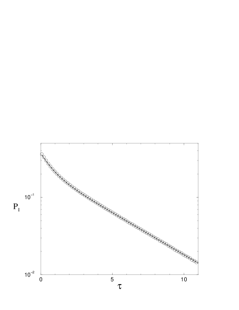
FIG. 2.: The interval size distribution $P_{I}(\tau)$ plotted on a semi-log scale as a function of $\tau$. The points are the numerical data while the line shows the approximate fit, Eq.(12).

Knowledge of $P_{I}(\tau)$ for all $\tau$ is needed to evaluate the integral in Eq.(9). A good fit to the numerical data can be obtained by writing $P_{I}(\tau)$ as the sum of just two exponentials,

$$P_{I}(\tau)=a_{1}e^{-\theta_{1}\tau}+a_{2}e^{-\theta_{2}\tau},$$ (12)

with $\theta_{1}=1/4$ and $a_{1}=0.2213$. The parameters $\theta_{2}$ and $a_{2}$ can be determined by imposing two constraints: (1) that $P_{I}(\tau)$ is normalized over the interval $[0,\infty]$ and (2) that it predicts the correct density of zeros[4] which is governed by the first moment of $P_{I}(\tau)$, $\rho=\sqrt{3}/{2\pi}=1/{\langle\tau\rangle}$. These conditions fix the unknown parameters to be $\theta_{2}=1.3254$ and $a_{2}=0.1521$, and this approximate expression is also plotted in Figure 2. It can be seen that the parameterised $P_{I}(\tau)$ fits the simulation data rather well over the whole range of $\tau$.

When this analytic expression for $P_{I}(\tau)$ is inserted into Eq.(9) one finds the following transcendental equation,

$$\frac{1}{r^{2\theta_{c}}}=\frac{a_{1}}{\theta_{1}-\theta_{c}}+\frac{a_{2}}{\theta_{2}-\theta_{c}},$$ (13)

which can be used to determine $\theta_{c}(r)$. The numerical solution of this equation is shown in Figure 3, together with the exponent values measured directly from the simulations. For $r$ close to $r_{c}$ it is hard to access the asymptotic regime numerically, hence the lack of data in this region of the plot. However, there is rather good agreement for all the values of $r$ considered. Note that with our parameterised expression for $P_{I}(\tau)$, the IIA correctly predicts both the $r\to 0$ limit and the critical value of $r$, namely $r_{c}=e^{-\pi/\sqrt{3}}$, where $\theta_{c}\to 0$. Thus, the analytic calculation confirms that the collapse exponent is non-universal and depends continuously on $r$. The inset in Figure 3 shows the behaviour of $\theta_{c}(r)$ for $r\to 0$, where the approximate analytic calculation and the simulation data appear to coincide. To leading order in $r$, Eq.(13) can be expanded to give

$$\theta_{c}=1/4-a_{1}\sqrt{r}+.\,.\,.\,.\,.$$ (14)

As only the first term on the right hand side of Eq.(13) contributes in this limit, the expansion is exact within the IIA, since both $\theta_{1}(=1/4)$ and $a_{1}$ are known exactly.

FIG. 3.: The collapse-time exponent $\theta_{c}$ as a function of $r$. The points are the numerical data, obtained from measuring the slopes of $P_{c}(T)$. The errors are of the same order as the size of the circles. The line is the analytic approximation determined from the solution of Eq.(13). The inset shows an expanded view of the main figure for $r$ close to zero where the simulation data and the approximate calculation appear to coincide.

Finally we point out an intriguing connection between the exponent $\theta_{c}$ and the persistence exponent of a randomly accelerated particle with ‘partial survival’ [14]. Consider the process $x(t)$ described by Eq.(1), and let the particle survive with probability $p$ each time its position, $x(t)$, crosses through zero. Working in the logarithmic time variable, $T=\ln t$, the probability that the particle survives for a time $T$ (in the stationary state) is

$$P_{\rm surv}(T)=\sum_{n=0}^{\infty}p^{n}\,P_{n}(T),$$ (15)

where $P_{n}(T)$ is the probability that the process has $n$ zero crossings in time $T$. We anticipate [14] that $P_{\rm surv}(T)\sim e^{-\theta(p)T}$ for $T\to\infty$, i.e. that the Laplace transform $\tilde{P}_{\rm surv}(s)$ will have a simple pole at $s=-\theta(p)$.

The Laplace transforms $\tilde{P}_{n}(s)$ were worked out, in terms of the Laplace transform $\tilde{P}_{I}(s)$ of the interval-size distribution, $P_{I}(\tau)$, within the IIA in [4]. Carrying out the sum over $n$ in Eq.(15) gives $\tilde{P}_{\rm surv}(s)$, and one finds a simple pole given by the condition $p\tilde{P}_{I}(s)=1$. Setting $s=-\theta(p)$ yields finally $p\int_{0}^{\infty}d\tau\,e^{\theta(p)\tau}\,P_{I}(\tau)=1$ as the equation determining $\theta(p)$. This equation has an identical form to Eq.(9) for $\theta_{c}$, suggesting that the collapse process with coefficient of restitution $r$ is in some sense equivalent to a randomly forced particle with survival probability $p=r^{2\theta_{c}}$ at each collision. As yet, however, we have been unable to establish this equivalence outside the IIA.

To summarize, we have studied the collapse-time distribution, $P_{c}(t)$, for a randomly-forced particle colliding inelastically with a boundary, in the regime $r<r_{c}$ where inelastic collapse occurs. We have shown that the distribution has a power-law tail, $P_{c}(t)\sim 1/t^{1+\theta_{c}}$, characterized by an exponent $\theta_{c}$ which varies continuously with $r$ for $0\leq r\leq r_{c}$. An analytical approach, based on the approximation that the intervals (in the variable $T=\ln t$) between zero crossings of a free, randomly accelerated particle can be treated as statistically independent, leads to results which are in good agreement with numerical simulations. We have also noted a formal similarity between Eq.(9), which determines $\theta_{c}$ within this approach, and the equivalent equation for the persistence exponent of a randomly accelerated particle with partial survival [14]. This similarity invites further study.

This work was supported by EPSRC (UK) under grant number GR/K53208.

REFERENCES

- [1] P. Langevin, Comptes Rendues 146, 530 (1908).
- [2] C. W. Gardiner, Handbook of Stochastic Methods for Physics, Chemistry and the Natural Sciences (Springer Verlag, Berlin, 1990).
- [3] B. Derrida, A. J. Bray and C. Godrechè, J. Phys. A 27, L357 (1994).
- [4] S. N. Majumdar, C. Sire, A. J. Bray and S. J. Cornell, Phys. Rev. Lett. 77, 2867 (1996); B. Derrida, V. Hakim and R. Zeitak, ibid., 2871.
- [5] J. Cardy, J. Phys. A 28, L19 (1995); E. Ben-Naim, Phys. Rev. E 53, 1566 (1996); M. Howard, J. Phys. A 29, 3437 (1996); S. J. Cornell and A. J. Bray, Phys. Rev. E 54, 1153 (1996).
- [6] B. Derrida, V. Hakim and V. Pasquier, Phys. Rev. Lett. 75, 751 (1995).
- [7] J. Krug, H. Kallabis, S. N. Majumdar, S. J. Cornell, A. J. Bray and C. Sire, Phys. Rev. E 56, 2702 (1997).
- [8] M. Marcos-Martin, D. Beysens, J-P. Bouchaud, C. Godrèche and I. Yekutieli, Physica A 214, 396 (1995).
- [9] B. Yurke, A. N. Pargellis, S. N. Majumdar and C. Sire, Phys. Rev. E 56, R40 (1997).
- [10] W. Y. Tam, R. Zeitak, K. Y. Szeto and J. Stavans, Phys. Rev. Lett. 78, 1588 (1997).
- [11] S. J. Cornell, M. R. Swift and A. J. Bray, Phys. Rev. Lett. 81, 1142 (1998).
- [12] For a review, see T. C. Lubensky, Solid-State-Communications, 102, 187 (1997).
- [13] D. R. M. Williams and F. C. MacKintosh, Phys. Rev. E 54, R9 (1996); M. R. Swift, M. Boamfǎ, S. J. Cornell and A. Maritan, Phys. Rev. Lett. 80, 4410 (1998); A. Puglisi, V. Loreto, U. Marini Bettolo Marconi, A. Petri and A. Vulpiani, Phys. Rev. Lett. 81, 3848 (1998); G. Peng and T. Ohta, cond-mat/9710119.
- [14] S. N. Majumdar and A. J. Bray, Phys. Rev. Lett. 81, 2626 (1998).
- [15] T. W. Burkhardt, J. Phys. A26, L1157 (1993).
- [16] We assume that the particle is injected from the origin at time with a velocity drawn from the scaling distribution. This assumption will allow us to treat the first interval on an equal footing with all the rest without changing the asymptotic behaviour of .
- [17] J. A. McFadden, IRE Transaction on Information Theory, IT-4, p.14 (1957).