Large$-N$ treatment of the Abrikosov transition at low temperatures.

Abstract

We investigate the influence of order parameter fluctuations on the transition between normal and mixed superconducting states at low temperatures. We show that in case of clean quasi-two-dimensional superconductors the transition can be described by the functional of the Ginzburg-Landau type. We consider the large$-N$ generalization of this functional and using the lowest Landau level approximation we get the large$-N$ equations which describe the phase transition. In case of physical dimensionality we found that the transition is of the first order. The fluctuations significantly affect the temperature dependence of the upper critical field.

]

I Introduction .

It is well known that the magnetic field penetrates type$-II$ superconductors through flux lines which form the Abrikosov lattice [1]. The theory of this mixed state was first developed by Abrikosov for temperatures close to $T_{c}$ [1], and then it was extended to all temperatures[2]. These theories ignore the fluctuations of the order parameter. It is a very good approximation for the conventional superconductors because in this case the order parameter fluctuations are important only in a very small region near the phase transition line. This happens because the Ginsburg numbers of the conventional superconductors are very small.

However for high$-T_{c}$ superconductors there are experiments which cannot be explained by the usual mean field theory. The upper critical field $H_{c2}$ at low temperatures significantly increases as temperature decreases instead of being approximately constant as follows from the mean field theory[3]. The Ginzburg numbers of high$-T_{c}$ superconductors are not very small, therefore one can suggest that this unusual behavior is due to the order parameter fluctuations. Also, it is important to understand the type of the phase transition (first order or second order), because in mean field approximation this transition is always of the second order, but the fluctuations can induce the first order phase transition. This happens, for example, in the model described in Ref.[4] and it was suggested to happen in the Abrikosov transition [5].

In the following we will consider the influence of the order parameter fluctuations on the transition between normal and mixed superconducting states in clean superconductors. We argue that in case of pure quasi-two-dimensional superconductors, when the magnetic field is applied along the low-conducting direction, even at low temperatures, this transition can be investigated by the effective functional of the Ginzburg-Landau (GL) type which contains imaginary time, because quantum fluctuations become important at low temperatures. Unfortunately, even having the effective functional one can hardly calculate the free energy exactly, which is typical for the critical phenomena problems. Therefore we modify the functional introducing $n-$ index to the fluctuating field and considering the large$-N$ limit. One should be careful in introducing of $n-$ index into this functional, because doing that in not a proper way one can get a model which does not have a solution in the form of the Abrikosov lattice[6]. Under the approximation when the mean field solution and fluctuations belong to the lowest Landau level (which is valid near the phase transition) we get the equations which describe the phase transition.

We show that in high enough dimensions (either $T=0,\,d>4$ or $T\not=0,\,d>6$) if the coupling constant is not too large the transition is of the second order. In this case the corrections from fluctuations do not modify mean field results essentially. In the physical case (d=3) the phase transition is always of the first order and the fluctuations significantly affect the phase transition line: the upper critical field increases as temperature decreases, and the curvature of this dependence is negative when the temperature is not too low (see later, Figs.4,5).

The paper is organized as follows: In Sec. II we describe the model. In Sec. III we derive the large-$N$ equations describing the phase transition. In Sec. IV we analyze the phase transition from the side of the normal state region. In Sec. V we simplify the large-$N$ equations making the lowest Landau level approximation. In Sec. VI we solve the large$-N$ equations in case of high dimensions. In Sec. VII we solve the large-$N$ equations in the physical case. In Sec. VIII we discuss the spectrum of the order parameter fluctuations. And we summarize our results in Sec. IX.

II Description of the model.

To analyze the transition to the superconducting state one can usually use GL functional. This functional is based on the expansion in the order parameter, so it is valid when the ratio of the order parameter and temperature ${\Delta/T}$ is small. In case when an external magnetic field close to $H_{c2}$ is applied, one can still use GL functional if ${\Delta/T}\ll 1$, but at low temperatures the expansion in this parameter becomes not possible. From the other hand the magnetic field produces a depairing effect, as temperature does, so one can try to expand in $\Delta$ because it is small compared with the magnetic field taken in the proper units. This was done in Ref.[7] and it was shown that the coefficient in ${|\phi|}^{4}$ term has a logarithmic singularity $\ln{1\over T},$ which means that the expansion in $\Delta$ is not possible at zero temperature. The appearance of this singularity can be easily understood physically: Indeed, if we consider a pair of electrons which move exactly parallel to the magnetic field, then the magnetic field does not affect them in the quasiclassical approximation. Therefore this singularity comes from the electrons moving parallel to the magnetic field or close to this direction, because the magnetic field does not produce a depairing effect for these electrons. The direct calculation of the coefficient of ${|\phi|}^{4}$ term shows, that indeed, the singularity comes from the momenta parallel to the magnetic field.

There is a way to avoid this problem if one considers a quasi-two-dimensional superconductor. Indeed, if the magnetic field is applied along the low-conducting direction, then due to the quasi-two-dimensional band structure there are no momenta parallel to the magnetic field. In this case it is possible to expand in $\Delta$ and get a functional of GL type. Unfortunately, the functional which arises does not match exactly the form of the usual GL functional. The difference is that the ${|\phi|}^{4}$ term becomes a nonlocal functional of $\phi$ fields with a range of “interaction” of the order of the magnetic length[7]. We hope that this difference is not crucial, and therefore we consider the model with a local ${|\phi|}^{4}$ term. The Lagrangian density of this model is

$${\cal L}=\phi^{*}\left(-{{D^{2}}\over{2m}}+\epsilon(\hat{p}_{\perp})+|\partial_{\tau}|+a\right)\phi+u{|\phi|}^{4}$$ (1)

$$+{{B^{2}}\over{8\pi}}-{{BH}\over{4\pi}},$$ (2)

where $D_{\mu}=\nabla_{\mu}-{{ie^{*}}\over c}A_{\mu}$ acts only in $x-y$ plane with the Abrikosov lattice, and $\epsilon_{\perp}={{p_{\perp}^{2}}\over{2m_{\perp}}}$ is the kinetic energy corresponding to the motion in the directions perpendicular to $x-y$ plane. In this Lagrangian $\phi$ is a function of coordinates and imaginary time because we want to consider the low-temperature quantum regime also. The operator $|\partial_{\tau}|$ means that in the Matsubara space this operator becomes $|\omega|.$ For the BCS model the coefficients in the Lagrangian (2) are

$$u\sim{1\over{p_{F}m_{e}}},\,\,{1\over{m_{\perp}}}\sim{{v_{F}^{2}}\over{\epsilon_{0}k_{a}^{2}}},\,\,\,a+\epsilon_{0}\sim\epsilon_{0}{{H-H_{c2}^{(0)}}\over{H_{c2}^{(0)}}},$$ (3)

where $\epsilon_{0}$ is the energy of the lowest Landau level, i.e. the lowest eigenvalue of ${{D^{2}}\over{2m}},$ $m_{e}$ is the electron mass, $H_{c2}^{(0)}$ is the critical field in the mean field approximation, and $k_{a}=t_{\|}/t_{\perp}$ is the anisotropy coefficient, which is the ratio of the in-plane electron hopping and the hopping in the direction perpendicular to the $x-y$ planes.

To make our approach systematic we will modify this model introducing $n-$index and considering the large$-N$ limit. The usual way to introduce $n-$index to ${|\phi|}^{4}$ term is

$$\phi^{*}\phi\phi^{*}\phi\to\phi^{*}_{n}\phi_{n}\phi^{*}_{m}\phi_{m}.$$ (4)

But it happens that the spectrum of fluctuations around the Abrikosov lattice is not positive definite in this case, i.e. the Abrikosov lattice is unstable[6]. (We will not consider the possibility of condensation into different n-components as in Ref.[6].) To understand the reason of this instability let us substitute $\phi=\phi_{0}+\phi_{1},$ where $\phi_{0}$ corresponds to the Abrikosov lattice and $\phi_{1}$ represents fluctuations around it, into ${|\phi|}^{4}$ term. Considering the simplest case when fluctuations are small, for ${|\phi|}^{4}$ term we have

$${|\phi|}^{4}=4\phi_{0}^{*}\phi_{0}\phi_{1}^{*}\phi_{1}+\phi_{0}^{*}\phi_{0}^{*}\phi_{1}\phi_{1}+\phi_{0}\phi_{0}\phi_{1}^{*}\phi_{1}^{*}+...,$$ (5)

where we wrote only the most interesting, quadratic in $\phi_{1}$ part. The spectrum of fluctuations corresponding to (5) was considered by Eilenberger [8], and it was found that it is positive definite, i.e. the Abrikosov lattice is stable. It is important that following to the Eilenberger approach one can see that these are the off-diagonal terms in (5) which make the lattice stable. But for ${|\phi|}^{4}$ term defined by (4) in the large$-N$ limit we have

$$\phi^{*}_{n}\phi_{n}\phi^{*}_{m}\phi_{m}=...+2\phi^{*}_{0}\phi_{0}\phi_{m}^{*}\phi_{m}+...,$$

so in this case we effectively drop out the off-diagonal terms and it leads to the unstable spectrum of fluctuations. Therefore we suggest the following modification of the model:

$$\phi^{*}\phi\phi^{*}\phi\to 2\phi^{*}_{n}\phi_{n}\phi^{*}_{m}\phi_{m}-\phi^{*}_{n}\phi_{n}^{*}\phi_{m}\phi_{m}.$$ (6)

In the large$-N$ limit for ${|\phi|}^{4}$ term now we have

$$4\phi_{0}^{*}\phi_{0}\phi_{n}^{*}\phi_{n}-\phi^{*}_{0}\phi^{*}_{0}\phi_{m}\phi_{m}-\phi_{0}\phi_{0}\phi^{*}_{m}\phi^{*}_{m},$$

which matches the form (5) after the redefinition $\phi_{m}\to i\phi_{m},\phi_{m}^{*}\to-i\phi_{m}^{*}.$ It is important that the second term in (6) should have the negative sign because otherwise the fluctuations around the Abrikosov lattice are unstable (from the above simple argument one cannot see that it should be negative). So the Lagrangian density of the model which we will consider is:

$${\cal L}=\phi^{*}_{n}\left(-{{D^{2}}\over{2m}}+\epsilon(p_{\perp})+|\partial_{\tau}|+a\right)\phi_{n}+{{B^{2}}\over{8\pi}}-{{BH}\over{4\pi}}$$ (7)

$$+{u\over N}(2\phi^{*}_{n}\phi_{n}\phi^{*}_{m}\phi_{m}-\phi^{*}_{n}\phi_{n}^{*}\phi_{m}\phi_{m}),$$ (8)

and the action and the partition function are

$$S=\int d\tau d^{d}x{\cal L},$$ (9)

$$Z=\int D\phi D\phi^{*}e^{-S}.$$ (10)

For simplicity, in the following we will neglect the fluctuations of the magnetic field, because in the lowest Landau level approximation it gives just a renormalization of $u$ term, [8, 9] moreover the high-$T_{c}$ superconductors are extremely type-II superconductors therefore even this renormalization is not essential.

III Large$-N$ equations.

The interaction term in the Lagrangian (8) can be decoupled with the help of a real field $\rho$ and a complex one $\Delta$

$${\cal L}=\phi^{*}_{n}\left({\cal E}+|\partial_{\tau}|+a+2\rho i\right)\phi_{n}+\Delta^{*}\phi_{n}\phi_{n}+\Delta\phi^{*}_{n}\phi^{*}_{n}$$ (11)

$$+{{B^{2}}\over{8\pi}}-{{BH}\over{4\pi}}+{N\over{2u}}\rho^{2}+{N\over u}\Delta^{*}\Delta,$$ (12)

where ${\cal E}=-{{D^{2}}\over{2m}}+\epsilon(p_{\perp})$ is the kinetic energy operator. From the form of this Lagrangian it is evident that the mean field value of $\rho$ should be imaginary, which is not a problem because one can always shift the contour of integration over $\rho$ in the complex plane. Therefore we simply redefine $\rho\to-i\rho$, because we will not consider the fluctuations of $\Delta$ and $\rho$ fields. Integrating over $N-1$ $\phi$ fields we get an effective Lagrangian

$${\cal L} =\phi^{*}_{0}\left({\cal E}+|\partial_{\tau}|+a+2\rho\right)\phi_{0}+\Delta^{*}\phi_{0}\phi_{0}+\Delta\phi_{0}^{*}\phi_{0}^{*}$$ (13)

$$-{N\over{2u}}\rho^{2}+{N\over u}\Delta^{*}\Delta+{{N-1}\over 2}Tr\ln G^{-1}+{{B^{2}}\over{8\pi}}-{{BH}\over{4\pi}}$$ , (14)

where the Green function $G$ satisfies the equation

$$\left[\begin{array}[]{cc}{\cal E}+|\omega|+a+2\rho&2\Delta\\ 2\Delta^{*}&{\cal E}^{*}+|\omega|+a+2\rho\end{array}\right]G({\bf r}_{1},{\bf r}_{2},\omega,p_{\perp})$$

$$\hskip 142.26378pt=\delta({\bf r}_{1}-{\bf r}_{2})$$ (15)

Taking the variation with respect to $\Delta,\rho,\phi_{0}$ and neglecting fluctuations of the magnetic field we get the large$-N$ equations

$$\left[\begin{array}[]{cc}{N\over 2u}\rho({\bf r})-\phi_{0}^{*}({\bf r})\phi_{0}({\bf r})&-{N\over u}\Delta({\bf r})-\phi_{0}({\bf r})\phi_{0}({\bf r})\\ -{N\over u}\Delta^{*}({\bf r})-\phi_{0}^{*}({\bf r})\phi_{0}^{*}({\bf r})&{N\over 2u}\rho({\bf r})-\phi_{0}^{*}({\bf r})\phi_{0}({\bf r})\end{array}\right]$$

$$\hskip 85.35826pt={{(N-1)T}\over V_{\perp}}\sum_{\omega,p_{\perp}}G({\bf r},{\bf r},\omega,p_{\perp}),$$ (16)

$$\left(-{{D^{2}}\over{2m}}+a+2\rho({\bf r})\right)\phi_{0}({\bf r})+2\Delta({\bf r})\phi_{0}^{*}({\bf r})=0,$$ (17)

where $V_{\perp}$ denotes the volume perpendicular to the planes with the Abrikosov lattice.

IV Normal state.

At temperatures higher than the temperature of the Abrikosov transition we have $\phi_{0}=0,\Delta=0$, and the equations (16,17) are reduced to

$${1\over{2u}}\rho={T\over{V_{\perp}}}\sum_{\omega,p_{\perp}}G(0,0,\omega,p_{\perp}),$$ (18)

where the limit $N\to\infty$ was taken. The Green function in this case is determined by

$$\left({\cal E}+a+2\rho+|\omega|\right)G({\bf r},0,\omega,p_{\perp})=\delta^{2}({\bf r}).$$ (19)

Under the approximation when $\phi$ field belongs to the lowest Landau level we can substitute $-{1\over{2m}}D^{2}=\epsilon_{0}$, where $\epsilon_{0}$ is the energy of the lowest Landau level and get

$${\rho\over{2u}}={{TH}\over{V_{\perp}\Phi_{0}}}\sum_{\omega,p_{\perp}}{1\over{\delta+|\omega|+\epsilon(p_{\perp})}}e^{-{1\over{\tilde{\epsilon}}}(\delta+\epsilon(p_{\perp})+|\omega|)},$$ (20)

where $\epsilon_{0}+2\rho+a=\delta$ and $\Phi_{0}={{2\pi c}\over{e^{*}}}.$ Also we introduced the ultra-violate cutoff $\tilde{\epsilon}.$ The advantage of this cutoff procedure is that the Green function with the cutoff can be written as

$${1\over{\delta+|\omega|+\epsilon(p_{\perp})}} e^{-{1\over{\tilde{\epsilon}}}(\delta+|\omega|+\epsilon(p_{\perp}))}$$ (21)

$$=\int_{1\over{\tilde{\epsilon}}}^{\infty} {{d\lambda}\over\lambda}e^{-\lambda(\delta+\epsilon(p_{\perp})+|\omega|)}.$$ (22)

The phase transition happens when the correlation length diverges, i.e. when $\delta\to 0$, therefore to find the phase transition line we should calculate the integrals in (20) for the case $T\gg\delta$ in which we have

$$\delta-a^{*}-\epsilon_{0}={{4uH}\over{\Phi_{0}}}\left({{m_{\perp}}\over{2\pi}}\right)^{{d_{\perp}}\over 2}$$

$$\hskip 28.45274pt\times\left\{\begin{array}[]{ccc}{\pi\over{3(d_{\perp}/2-2)}}{\tilde{\epsilon}}^{d_{\perp}/2-2}\,\,T^{2},\,\,\,d_{\perp}>4\vspace{0.4cm}\\ \pi^{d_{\perp}/2-1}\,\xi\,\,T^{d_{\perp}/2},\,\,\,\,2<d_{\perp}<4\vspace{0.4cm}\\ \Gamma(1-d_{\perp}/2)\,\delta^{d_{\perp}/2-1}\,\,T,\,\,\,\,d_{\perp}<2,\end{array}\right.$$ (23)

where $a^{*}$ is the “mass” term $a$ renormalized by the quantum fluctuations

$$a^{*}=a+{{8uH}\over{\Phi_{0}\pi d_{\perp}}}\left({{m_{\perp}{\tilde{\epsilon}}}\over{2\pi}}\right)^{d_{\perp}/2},$$ (24)

$\xi$ is a constant

$$\xi=\int_{0}^{\infty}{{d\lambda}\over{\lambda^{d_{\perp}/2}}}(\coth\lambda-{1\over\lambda}),$$

and we introduced a notation for the dimensions perpendicular to $x-y$ planes $d_{\perp}=d-2.$ One can see that in high dimensions $d_{\perp}>4$ the correction to the phase transition line is analytical in $T,$ therefore it does not change the mean field result essentially. When $2<d_{\perp}<4$ the correction is non-analytical. Substituting $a^{*}+\epsilon_{0}\sim\epsilon_{0}(H-H_{c2}^{(0)*})/H_{c2}^{(0)},$ for the last case we have

$$H_{c2}-H_{c2}^{(0)*}\sim-T^{d_{\perp}/2},\,\,\,\,2<d_{\perp}<4,$$

where $H_{c2}^{(0)*}$ is the mean field upper critical field renormalized by the quantum fluctuations (see (24)). In the physical case $d_{\perp}=1$ one can see that the r.h.s of (23) diverges as ${1\over{\sqrt{\delta}}}$ when $\delta\to 0.$ In this case (23) can be written in the form

$${{\delta-a^{*}-\epsilon_{0}}\over{\epsilon_{0}}}=2\kappa_{G}{T\over{\epsilon_{0}}}\sqrt{{{\epsilon_{0}}\over\delta}},$$ (25)

where $\kappa_{G}$ is the Ginzburg number

$$\kappa_{G}={{2uH}\over{\sqrt{\epsilon_{0}}\Phi_{0}}}\left({{m_{\perp}}\over 2}\right)^{1\over 2}.$$ (26)

Using (3) we can estimate $\kappa_{G}\sim{{k_{a}}\over{p_{F}^{2}S}}$, where $S$ is the area corresponding to the unit flux $\Phi_{0}.$ By the order of magnitude $S\sim\xi^{2}$, where $\xi$ is the coherence length. In case when $\kappa_{G}$ is small one can find the qualitative crossover line between the Gaussian region (where the u-term is not important) and the non-Gaussian region (when it becomes important). In the Gaussian regime one can neglect the r.h.s. in (25) getting $\delta\approx a^{*}+\epsilon_{0}.$ The crossover line corresponds to the situation when the r.h.s of (25) becomes of the same order with the l.h.s., so that we have $\delta\sim(\sqrt{\epsilon_{0}}\kappa_{G}T)^{2/3}$ or

$${{H_{cr}-H_{c2}^{(0)*}}\over{H_{c2}^{(0)}}}\sim-\left({{\kappa_{G}T}\over{\epsilon_{0}}}\right)^{2/3},$$ (27)

where $H_{cr}$ is the magnetic field corresponding to the crossover from the Gaussian to the non-Gaussian regime. The fact that one cannot reach the ordered state going from the normal state gives us a hint that the transition to the ordered state is not continues.

V Ordered state.

We will solve Eqs.(15,16,17) under the approximation when the mean field $\phi_{0}$ and the fluctuations around it belong to the lowest Landau level. Also, as usually, we will consider a lattice with the triangular symmetry. Therefore, following to the Eilenberger notations[8], we take $\phi_{0}$ to be proportional to

$$\phi({\bf r}|0)=(2\eta)^{1\over 4}\sum_{p}e^{{{2\pi}\over\eta}\left(-{1\over 2}(y+p\eta)^{2}+ip\eta(x+{1\over 2}p\xi)\right)},$$ (28)

where $\eta,\xi$ are components of the vectors which determine the unit cell

$${\bf r}_{I}=(1,0),\,\,\,{\bf r}_{II}=(\xi,\eta)=({1\over 2},{{\sqrt{3}}\over 2}).$$ (29)

In the above formulas we measure all distances in the distances between the vertices $l$, which is related to the magnetic field by

$$\Phi_{0}=H{{\sqrt{3}}\over 2}l^{2}.$$ (30)

Applying the magnetic translation operator to (28) we can get a complete basis of functions belonging to the lowest Landau level

$$\phi({\bf r}|{\bf r}_{0})=e^{2\pi i{{y_{0}}\over\eta}x}\phi({\bf r}+{\bf r}_{0}|0),$$ (31)

which obey the orthogonality relation

$$\int d^{2}r\,\phi^{*}({\bf r}|{\bf r_{1}})\phi({\bf r}|{\bf r}_{2})=\eta^{2}\delta^{2}({\bf r}_{1}-{\bf r}_{2}).$$ (32)

Restricting our solution to the lowest Landau level we artificially decrease the space of solutions of Eqs.(15,16,17), therefore to have a solution we should decrease the space of equations projecting them on the lowest Landau level. The way to do that becomes evident if we consider the Schroedinger equation which corresponds to the Green function equation (15)

$$\left(-{{D^{2}}\over{2m}}+\epsilon(p_{\perp})+|\omega|+a+2\rho\right)\phi+2\Delta\phi^{*}=E\phi.$$ (33)

Indeed, to project this equation on the lowest Landau level one should multiply it by $\phi^{*}({\bf r}|{\bf r}_{0})$ and integrate over ${\bf r}.$ Introducing the following notations for the matrix elements of $\rho$ and $\Delta$

$$\int d^{2}r\,\phi^{*}({\bf r}|{\bf r}_{1})\rho({\bf r})\phi({\bf r}|{\bf r}_{2})=\eta^{2}\rho_{{\bf r}1,{\bf r}2},$$ (34)

$$\int d^{2}r\,\phi^{*}({\bf r}|{\bf r}_{1})\Delta({\bf r})\phi^{*}({\bf r}|{\bf r}_{2})=\eta^{2}\Delta_{{\bf r}1,{\bf r}2},$$ (35)

and presenting $\phi$ as

$$\phi({\bf r})=\int d^{2}r_{0}a({\bf r}_{0})\phi({\bf r}|{\bf r}_{0}),$$ (36)

we get

$$\left(\epsilon_{0}+\epsilon(p_{\perp})+|\omega|+a\right)a({\bf r}_{1})$$ (37)

$$+2\int d^{2}r_{2}\,a({\bf r}_{2}) (\rho_{{\bf r}1,{\bf r}2}+\Delta_{{\bf r}1,{\bf r}2})=E\,a({\bf r}_{1}).$$ (38)

From the symmetry of this problem we expect that $\rho$ is a periodic function, and $\Delta$ is a quasiperiodic one (that means periodic up to the phase), therefore the only matrix elements which are allowed by the translational symmetry are

$$\rho_{{\bf r}1,{\bf r}2}=\rho_{{\bf r}1}\delta^{2}({\bf r}_{1}-{\bf r}_{2}),$$ (39)

$$\Delta_{{\bf r}1,{\bf r}2}=\Delta_{{\bf r}1}\delta^{2}({\bf r}_{1}+{\bf r}_{2}).$$ (40)

Now we can find the eigenfunctions and the energy levels of (33):

$$u_{\pm}({\bf r})={1\over{\sqrt{2}}}e^{i{{\theta(r)}\over 2}}\left(e^{ikz}\phi({\bf r}|{\bf r}_{0})\pm e^{-ikz}\phi({\bf r}|-{\bf r}_{0})\right),$$ (41)

$$v_{\pm}({\bf r})={1\over{\sqrt{2}}}e^{i{{\theta(r)}\over 2}}\left(ie^{ikz}\phi({\bf r}|{\bf r}_{0})\mp ie^{-ikz}\phi({\bf r}|-{\bf r}_{0})\right),$$ (42)

$$E_{\pm}({\bf r},p_{\perp},\omega)=\epsilon_{0}+\epsilon_{\perp}(p_{\perp})+a+2(\rho_{\bf r}\pm|\Delta_{\bf r}|),$$ (43)

where

$$e^{i\theta({\bf r})}={{\Delta_{\bf r}}\over{|\Delta_{\bf r}|}}.$$

One can see that there are two energy branches which are denoted by the subscript $\pm$, and there are two eigenfunctions $u$ and $v$ for each energy level.

The green function (15) can be expressed through the eigenfunctions (41,42)

$$G({\bf r}_{1},{\bf r}_{2},p_{\perp},\omega)$$ (44)

$$={1\over{2\eta^{2}l^{2}}}\sum_{s,j} \int^{\prime}d^{2}r_{0}{{\Psi_{j,s}({\bf r}_{1}|{\bf r}_{0})\Psi_{j,s}^{\dagger}({\bf r}_{2}|{\bf r}_{0})}\over{E_{j}({\bf r}_{0},p_{\perp},\omega)}},$$ (45)

where the index $j=+,-$ denotes the spectrum branch and $s=u,v$ denotes the type of function:

$$\Psi_{\pm,u}=\left(\begin{array}[]{cc}u_{\pm}\\ u^{*}_{\pm}\end{array}\right),\Psi_{\pm,u}^{\dagger}=\left(u_{\pm}^{*}\,\,u_{\pm}\right),$$ (48)

$$\Psi_{\pm,v}=\left(\begin{array}[]{cc}v_{\pm}\\ v^{*}_{\pm}\end{array}\right),\Psi_{\pm,v}^{\dagger}=\left(v_{\pm}^{*}\,\,v_{\pm}\right).$$ (51)

The prime under the integral in (45) denotes the integration over the half of the unit cell. From the Goldstone theorem we expect a singularity in (45) at the minimal energy, i.e. $E_{-}(0,0,0)=0.$ This condition is consistent with the equation (17) if we take

$$\phi_{0}=i\sqrt{bN}\phi({\bf r}|0),$$

where $b$ is a real positive number. Indeed, projecting (17) on the lowest Landau level we get

$$\epsilon_{0}+a+2(\rho_{0}-\Delta_{0})=0,$$ (52)

which is the same with $E_{-}(0,0,0)=0.$

Now, to get a closed system of equations, we should take the matrix elements of the equation (16). Using the addition theorem of the Eilenberger functions [8].

$$\phi({\bf r}|{\bf r}_{1})\phi({\bf r}|{\bf r}_{2})={1\over{\sqrt{2}}}\biggl{[}\tilde{\phi}({\bf r}|({\bf r}_{1}+{\bf r}_{2})/2)\tilde{\phi}(({\bf r}_{1}-{\bf r}_{2})/2|0)\biggr{.}$$

$$+\tilde{\phi}({\bf r}|({\bf r}_{1}+{\bf r}_{2}+{\bf r}_{I})/2)\tilde{\phi}(({\bf r}_{1}-{\bf r}_{2})/2|{\bf r}_{I}/2)\biggr{]},$$

where $\tilde{\phi}$ is defined by (28,31) with the difference $\tilde{\bf r}_{II}={1\over 2}{\bf r}_{II}$, we get

$$-{T\over{2\eta^{2}V_{\perp}l^{2}}}\sum_{p_{\perp},\omega,j}\int^{\prime}d^{2}r_{0}{{\mathop{\rm sgn}\nolimits j\,\,e^{i\theta(r_{0})}}\over{E_{j}({\bf r}_{0},p_{\perp},\omega)}}\biggl{[}\tilde{\phi}^{*}({\bf r}|0)\tilde{\phi}({\bf r}_{0}|0)$$

$$+\tilde{\phi}^{*}({\bf r}|{\bf r}_{I}/2)\tilde{\phi}({\bf r}_{0}|{\bf r}_{I}/2)\biggr{]}={{\Delta_{\bf r}}\over u}-bQ({\bf r})$$ (53)

$$-{T\over{2\eta^{2}V_{\perp}l^{2}}}\sum_{p_{\perp},\omega,j}\int^{\prime}d^{2}r_{0}{{K({\bf r}-{\bf r}_{0})+K({\bf r}+{\bf r}_{0})}\over{E_{j}({\bf r}_{0},p_{\perp},\omega)}}$$

$$\hskip 113.81102pt=-{{\rho_{\bf r}}\over u}+bK({\bf r}),$$ (54)

where

$$\mathop{\rm sgn}\nolimits j=\left\{\begin{array}[]{c}1\,\,\,\,{\rm for\,(+)\,branch}\\ -1\,\,\,\,{\rm for\,(-)\,branch}\end{array}\right.,$$ (55)

and we introduced the following functions

$$K({\bf r})=\left|\tilde{\phi}({\bf r}/2|0)\right|^{2}+\left|\tilde{\phi}({\bf r}/2|{\bf r}_{I}/2)\right|^{2},$$ (56)

$$Q({\bf r})={1\over 2}\left(\tilde{\phi}^{*}({\bf r}|0)\tilde{\phi}(0|0)+\tilde{\phi}^{*}({\bf r}|{\bf r}_{I}/2)\tilde{\phi}(0|{\bf r}_{I}/2)\right).$$ (57)

From Eq.(53) one can see that $\Delta_{\bf r}$ is a linear combination of the functions $\tilde{\phi}^{*}({\bf r}|0)$ and $\tilde{\phi}^{*}({\bf r}|{\bf r}_{I}/2).$ Therefore, presenting $\Delta_{\bf r}$ as

$$\Delta_{\bf r}={1\over 2}\left(\Delta_{1}\tilde{\phi}^{*}({\bf r}|0)\tilde{\phi}(0|0)+\Delta_{2}\tilde{\phi}^{*}({\bf r}|{\bf r}_{I}/2)\tilde{\phi}(0|{\bf r}_{I}/2)\right),$$ (58)

from (53) we get two equations on $\Delta_{1},\Delta_{2}$

$${T\over{\eta^{2}V_{\perp}l^{2}}}\sum_{p_{\perp},\omega,j}\int d^{2}r_{0}{{\mathop{\rm sgn}\nolimits j\,e^{i\theta(r_{0})}}\over{E_{j}({\bf r}_{0},p_{\perp},\omega)}}\tilde{\phi}({\bf r}_{0}|0)$$ (59)

$$=\tilde{\phi}(0|0)\left(b-{{\Delta_{1}}\over u}\right)$$ (60)

$${T\over{\eta^{2}V_{\perp}l^{2}}}\sum_{p_{\perp},\omega,j}\int d^{2}r_{0}{{\mathop{\rm sgn}\nolimits j\,e^{i\theta(r_{0})}}\over{E_{j}({\bf r}_{0},p_{\perp},\omega)}}\tilde{\phi}({\bf r}_{0}|{\bf r}_{I}/2)$$ (61)

$$=\tilde{\phi}(0|{\bf r}_{I}/2)\left(b-{{\Delta_{2}}\over u}\right)$$ (62)

From the symmetry of the problem we expect that $\Delta_{\bf r}$ is not only quasiperiodic (which is evident from (58)), but it is also quasisymmetric under rotations on $\pi/3.$ The later property is satisfied only when $\Delta_{1}=\Delta_{2}.$ But taking $\Delta_{1}=\Delta_{2}$ we should prove that Eqs.(60,62) become linear dependent. One can check that it happens indeed, multiplying (60) by $\tilde{\phi}(0|{1\over 2}{\bf r}_{I})$ and (62) by $-\tilde{\phi}(0|0)$, adding them, and using that the function

$$D\equiv\left(\tilde{\phi}^{*}({\bf r}|0)\tilde{\phi}(0|0)+\tilde{\phi}^{*}({\bf r}|{1\over 2}{\bf r}_{I})\tilde{\phi}(0|{1\over 2}{\bf r}_{I})\right)$$ (63)

$$\times\left(\tilde{\phi}({\bf r}|0)\tilde{\phi}(0|{1\over 2}{\bf r}_{I})-\tilde{\phi}({\bf r}|{1\over 2}{\bf r}_{I})\tilde{\phi}(0|0)\right)$$ (64)

transforms under rotation on $\pi/3$ as

$$D\to D\,\,e^{-i{{2\pi}\over 3}}\,\,\,\,{\rm when}\,\,x+iy\to(x+iy)e^{i\pi/3}.$$ (65)

Finally we get the following system of equations:

$${T\over{2\eta^{2}V_{\perp}l^{2}}}\sum_{p_{\perp},\omega,j}\int d^{2}r{{\mathop{\rm sgn}\nolimits j}\over{E_{j}({\bf r},p_{\perp},\omega)}}|Q({\bf r})|$$ (66)

$$=\left(b-{\Delta\over u}\right)Q(0),$$ (67)

$${T\over{2\eta^{2}V_{\perp}l^{2}}}\sum_{p_{\perp},\omega,j}\int d^{2}r_{0}{1\over{E_{j}({\bf r}_{0},p_{\perp},\omega)}}K({\bf r}_{0}-{\bf r})$$ (68)

$$={{\rho_{\bf r}}\over u}-bK({\bf r}),$$ (69)

$$E_{\pm}({\bf r},p_{\perp},\omega)=\epsilon_{0}+a+\epsilon(p_{\perp})+|\omega|+2\left(\rho_{\bf r}\pm\Delta|Q({\bf r})|\right),$$ (70)

$$E_{-}(0,0,0)=0.$$ (71)

VI Solution of the large$-N$ equations in high dimensions.

In high enough dimensions we can expand Eqs.(67,69) in $\rho,\Delta.$ This expansion is possible when either $d_{\perp}>4$, $T\not=0$ or $d_{\perp}>2$, $T=0.$ In these cases one can write

$${{Tu}\over{2\eta^{2}V_{\perp}l^{2}}}\sum_{p_{\perp},\omega}{1\over{\epsilon(p_{\perp})+|\omega|+x}}=\alpha-\beta x.$$ (72)

From Eqs.(67,69) we get

$$-4\beta\Delta\int d^{2}r\,\,Q^{*}({\bf r})Q({\bf r})=(bu-\Delta)Q(0),$$ (73)

$$2\int d^{2}r_{0}\,\,\left(\alpha-\beta(\epsilon_{0}+a+2\rho({\bf r}_{0}))\right)K({\bf r}_{0}-{\bf r})$$ (74)

$$=\rho_{\bf r}-buK({\bf r}).$$ (75)

The first equation (73) can be solved immediately giving

$$\Delta={{bu}\over{1-2\beta\eta}}.$$ (76)

The second equation (75) can be solved by the Fourier transformation which we define as

$$K({\bf r})=\sum_{k}e^{-i{\bf k}{\bf r}}K({\bf k}),$$ (77)

where due to the periodicity of $K({\bf r})$ the vector ${\bf k}$ should have the following discrete values

$${\bf k}={\bf k}_{1}n_{1}+{\bf k}_{2}n_{2},$$ (78)

$${\bf k}_{1}=2\pi(0,-{2\over{\sqrt{3}}})\,\,\,\,,{\bf k}_{2}=2\pi(1,-{1\over{\sqrt{3}}}),$$ (79)

where $n_{1},n_{2}$ are integers. The Fourier transformation of $K({\bf r})$ can be done analytically

$$K({\bf k})=e^{-{{2\pi}\over{\sqrt{3}}}(n_{1}^{2}+n_{1}n_{2}+n_{2}^{2})}.$$ (80)

Defining the Fourier transformation for $\rho_{\bf r}$ by the same rule, from Eq.(75) we get

$$\rho({\bf k})={{4(\alpha-\beta(\epsilon_{0}+a))\eta\,\,\delta_{{\bf k},0}+buK({\bf k})}\over{1+4\beta\eta K({\bf k})}}.$$ (81)

Substitution of (76,81) to (71) gives the equation for the condensate density $b$

$$2bu\left({{Q(0)}\over{1-2\beta\eta}}-\sum_{k}{{K({\bf k})}\over{1+4\eta\beta K({\bf k})}}\right)={{\epsilon_{0}+a+8\eta\alpha}\over{1+8\eta\beta}}.$$ (82)

Using this equation we can present the spectrum as

$$E_{\pm}({\bf r})=bu\left(\sum_{k}{{K({\bf k}){\,\,e^{i{\bf k}{\bf r}}}}\over{1+4\beta\eta K({\bf k})}}\pm{{|Q({\bf r})|}\over{1-2\beta\eta}}\right)-({\bf r}=0).$$ (83)

One can check that this spectrum is positive definite which means that our solution is stable. The transition point can be found from (82) taking $b=0$

$$\epsilon_{0}+a_{c}=-8\eta\alpha,$$ (84)

where $a_{c}$ means the critical value for $a.$ The same result can be obtained from (20). We expect to have a nonzero $b$ in the ordered state when $a<a_{c}.$ But Eq.(82) has positive solutions for $b$ (and $b$ was chosen to be positive) only when the expression in the parenthesis on the l.h.s. of (82) is negative. Numerical calculation of this expression gives that it is negative only when

$$\beta<\beta_{c},$$ (85)

where $\beta_{c}=0.112.$ When the condition (85) is satisfied the condensate density $b$ can have any small values as a function of $a$. Therefore in that case the phase transition is of the second order. Note that the expansion (72) is valid only when $\Delta,\rho,b\ll\epsilon_{0}.$ When the phase transition is of the second order this condition can be always satisfied if we close enough to the phase transition line. Therefore the absence of the solution when $\beta>\beta_{c}$ in fact means that the transition is not continues.

Let us now summarize the results of this section where we were interested in the cases $d>4,T\not=0$ and $d>2,T=0$ : When the interaction constant is not too strong (condition (85)) the phase transition is of the second order. If the condition (85) is not satisfied then the transition between the normal to the ordered states cannot be continues.

VII Physical case

Let us consider the physical case $d=3$ ($d_{\perp}=1$). Taking the integral over $p_{\perp}$ and summing over $\omega$ in (67,69) we get

$$t\int d^{2}r\,\,\biggl{[}\sqrt{T}\Bigl{(}f(\epsilon_{+}({\bf r})/T)-f(\epsilon_{-}({\bf r})/T)\Bigr{)}$$ (86)

$$-{2\over{\sqrt{\pi}}}\left(\sqrt{\epsilon_{+}({\bf r})}-\sqrt{\epsilon_{-}({\bf r})}\right)\biggr{]}|Q({\bf r})|$$ (87)

$$=(bu-\Delta)Q(0)$$ (88)

$$t\int d^{2}r_{0}\,\,\biggl{[}\sqrt{T}\Bigl{(}f(\epsilon_{+}({\bf r}_{0})/T)-f(\epsilon_{-}({\bf r}_{0})/T)\Bigr{)}$$ (89)

$$-{2\over{\sqrt{\pi}}}\left(\sqrt{\epsilon_{+}({\bf r}_{0})}-\sqrt{\epsilon_{-}({\bf r}_{0})}\right)\biggr{]}K({\bf r}_{0}-{\bf r})$$ (90)

$$=\rho_{\bf r}-buK({\bf r})-{{4\sqrt{3\tilde{\epsilon}}}\over\pi}t,$$ (91)

where

$$\epsilon_{\pm}({\bf r})=\epsilon_{0}+a+2(\rho_{r}\pm\Delta|Q({\bf r})|),$$ (92)

$$f(x)=\int_{0}^{\infty}{{d\lambda}\over{\sqrt{\lambda}}}e^{-\lambda x}\left(\coth\pi\lambda-{1\over{\pi\lambda}}\right),$$ (93)

and

$$t={{u\sqrt{m_{\perp}}}\over{2\eta^{2}l^{2}\sqrt{2\pi}}}.$$ (94)

It is convenient to introduce the following dimensionless variables

$$T=\epsilon_{0}\kappa_{G}^{2}T^{\prime},\,\,\,\Delta=\epsilon_{0}\kappa_{G}^{2}\Delta^{\prime},$$ (95)

$$\rho=\epsilon_{0}\kappa_{G}^{2}\rho^{\prime},\,\,\,bu=\epsilon_{0}\kappa_{G}^{2}b^{\prime},$$ (96)

$$\epsilon_{0}+a=\epsilon_{0}\kappa_{G}^{2}a^{\prime},$$ (97)

where $\kappa_{G}$ is the Ginzburg number (26). In these new variables the equations do not contain $\kappa_{G}$ explicitly:

$$k\int d^{2}r\,\,\biggl{[}\sqrt{T^{\prime}}\Bigl{(}f(\epsilon_{+}^{\prime}({\bf r})/T^{\prime})-f(\epsilon_{-}^{\prime}({\bf r})/T^{\prime})\Bigr{)}$$ (98)

$$-{2\over{\sqrt{\pi}}}\left(\sqrt{\epsilon_{+}^{\prime}({\bf r})}-\sqrt{\epsilon_{-}^{\prime}({\bf r})}\right)\biggr{]}|Q({\bf r})|$$ (99)

$$=(b^{\prime}-\Delta^{\prime})Q(0),$$ (100)

$$k\int d^{2}r\,\,\biggl{[}\sqrt{T^{\prime}}\Bigl{(}f(\epsilon_{+}^{\prime}({\bf r}_{0})/T^{\prime})-f(\epsilon_{-}^{\prime}({\bf r}_{0})/T^{\prime})\Bigr{)}$$ (101)

$$-{2\over{\sqrt{\pi}}}\left(\sqrt{\epsilon_{+}^{\prime}({\bf r}_{0})}-\sqrt{\epsilon_{-}^{\prime}({\bf r}_{0})}\right)\biggr{]}K({\bf r}_{0}-{\bf r})$$ (102)

$$=\rho_{\bf r}^{\prime}-b^{\prime}K({\bf r})-{{4\sqrt{3\tilde{\epsilon}}}\over{\pi\epsilon_{0}}}t,$$ (103)

where $k=1/(2\sqrt{3\pi})$ is a numerical constant. Note that the third term on the r.h.s. of Eq.(103) can be absorbed into renormalization of $\rho^{\prime}$ and $a^{\prime}$

$$\rho^{\prime}\to\rho^{\prime}+{{4\sqrt{3\tilde{\epsilon}}}\over{\pi\epsilon_{0}}}t$$

$$a^{\prime}\to a^{\prime}-{{8\sqrt{3\tilde{\epsilon}}}\over{\pi\epsilon_{0}}}t.$$

This corresponds to the renormalization of the external magnetic field by the quantum fluctuations as in (24). Eq.(103) is an integral equation with the kernel

$$K({\bf r})=\sum_{n_{1},n_{2}}e^{-{{2\pi}\over{\sqrt{3}}}(n_{1}^{2}+n_{1}n_{2}+n_{2}^{2})}e^{-2\pi i({\bf k}_{1}n_{1}+{\bf k}_{2}n_{2}){\bf r}},$$ (104)

where ${\bf k}_{1},{\bf k}_{2}$ were defined in (79). To simplify the problem we will take an approximate expression for this kernel leaving only zeroth and first harmonics:

$$K({\bf r})=2+\gamma\biggl{[}\cos 2\pi{{2y}\over{\sqrt{3}}}+\cos 2\pi\left(x+{y\over{\sqrt{3}}}\right)$$ (105)

$$+\cos 2\pi\left(x-{y\over{\sqrt{3}}}\right)\biggr{]},$$ (106)

where $\gamma=4e^{-2\pi/\sqrt{3}}\approx 0.1063.$ It seems to be a good approximation because the contribution from higher harmonics to (104) decreases exponentially with the harmonic order. For example the contribution from the second harmonic is less then $0.1\%$ of the first one. Presenting $\rho_{\bf r}^{\prime}$ in the form

$$\rho_{\bf r}^{\prime}=\rho_{0}+\gamma\rho_{1}\biggl{[}\cos 2\pi{{2y}\over{\sqrt{3}}}+\cos 2\pi\left(x+{y\over{\sqrt{3}}}\right)$$ (107)

$$+\cos 2\pi\left(x-{y\over{\sqrt{3}}}\right)\biggr{]},$$ (108)

we get the following system of equations

$$2k\int d^{2}r\,\,\biggl{[}\sqrt{T^{\prime}}\Bigl{(}f(\epsilon_{+}^{\prime}({\bf r})/T^{\prime})+f(\epsilon_{-}^{\prime}({\bf r})/T^{\prime})\Bigr{)}$$ (109)

$$-{2\over{\sqrt{\pi}}}\left(\sqrt{\epsilon_{+}^{\prime}({\bf r})}+\sqrt{\epsilon_{-}^{\prime}({\bf r})}\right)\biggr{]}=\rho_{0}-2b^{\prime},$$ (110)

$$k\int d^{2}r\,\,\biggl{[}\sqrt{T^{\prime}}\Bigl{(}f(\epsilon_{+}^{\prime}({\bf r})/T^{\prime})+f(\epsilon_{-}^{\prime}({\bf r})/T^{\prime})\Bigr{)}$$ (111)

$$-{2\over{\sqrt{\pi}}}\left(\sqrt{\epsilon_{+}^{\prime}({\bf r})}+\sqrt{\epsilon_{-}^{\prime}({\bf r})}\right)\biggr{]}\cos 2\pi{{2y}\over{\sqrt{3}}}=\rho_{1}-b^{\prime},$$ (112)

$$k\int d^{2}r\,\,\biggl{[}\sqrt{T^{\prime}}\Bigl{(}f(\epsilon_{+}^{\prime}({\bf r})/T^{\prime})-f(\epsilon_{-}^{\prime}({\bf r})/T^{\prime})\Bigr{)}$$

$$-{2\over{\sqrt{\pi}}}\left(\sqrt{\epsilon_{+}^{\prime}({\bf r})}-\sqrt{\epsilon_{-}^{\prime}({\bf r})}\right)\biggr{]}|Q({\bf}r)|=(b^{\prime}-\Delta^{\prime})Q(0),$$ (113)

$$\epsilon_{\pm}^{\prime}({\bf r})=2\Bigl{(}\rho_{1}\gamma\,\,s(x,y)+\Delta^{\prime}(Q(0)\pm|Q({\bf r})|)\Bigr{)}$$ (114)

$$\rho_{0}=\Delta^{\prime}Q(0)-3\rho_{1}\gamma-a^{\prime}/2$$ (115)

where

$$s(x,y)=\cos 2\pi{{2y}\over{\sqrt{3}}}+\cos 2\pi\left(x+{y\over{\sqrt{3}}}\right)$$ (116)

$$+\cos 2\pi\left(x-{y\over{\sqrt{3}}}\right)-3.$$ (117)

Eq.(115) follows from Eq.(71). Note that the spectrum (114) contains only $\Delta^{\prime}$ and $\rho_{1}$, therefore combining Eqs.(112,113) to get rid of $b^{\prime}$ on the right hand sides we get a closed equation on $\Delta^{\prime}$ and $\rho_{1}.$ Therefore taking a given $\Delta^{\prime}$ we can solve this equation for $\rho_{1}.$ Then, knowing $\Delta^{\prime}$ and $\rho_{1}$ we can find all the other parameters $b^{\prime},a^{\prime},\rho_{0}.$ In Figs. 1-3 we present the graphs of $\rho_{1},b^{\prime},a^{\prime}$ as functions of $\Delta^{\prime}$ for different temperatures. Note that for large $\Delta^{\prime}$ the fluctuation contribution is small and one should have the mean field results:

$$b^{\prime}=\rho_{1}=\Delta^{\prime},\,\,\,a^{\prime}=-2Q(0)b^{\prime},\,\,\,\,\Delta^{\prime}\to\infty.$$ (118)

One can see that the graphs on Figs.1-3 begin to approach this asymptotics.

Let us start the analysis of these graphs from the low-temperature case (see Fig. 1): One can see that $a^{\prime}$ first increases as $\Delta^{\prime}$ decreases (as one should expect from the mean field theory), but then it decreases. The extremum point corresponds to the first order phase transition.

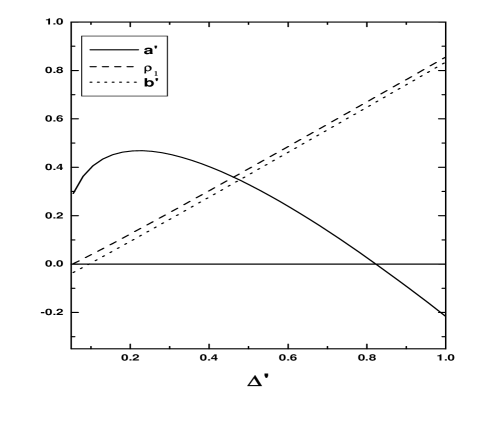
FIG. 1.: Solution of Eqs.(110-115) at temperature $T^{\prime}=0.1.$ The extremum in $a^{\prime}$ corresponds to the first order phase transition. Note that the condensate density $b^{\prime}$ is finite at this point.

At high temperatures the behavior is different (see Fig. 3): Going from large $\Delta^{\prime}$ we see that in this case first the condensate density $b^{\prime}$ becomes zero, and then there is an extremum in $a^{\prime}.$ In our approach it was chosen that $b^{\prime}>0,$ therefore the point $b^{\prime}=0$ corresponds to the first order phase transition. We call this transition also first order one because it is still discontinues in $\rho$ and $\Delta.$ So, the transition is of the first order for all temperatures, but at low temperatures it corresponds to the extremum of $a^{\prime}$, while at high temperatures it corresponds to depleting of the condensate density to zero. This change in the kind of the first order phase transition takes place at $T^{\prime}=T^{*}\approx 2.6.$

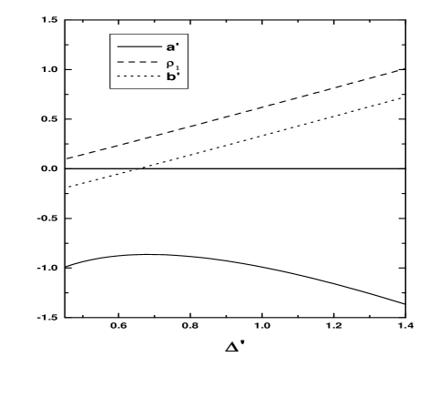
FIG. 2.: Solution of Eqs.(110-115) at temperature $T^{\prime}=2.0$ The condensate density $b^{\prime}$ is close to zero at the point of extremum of $a^{\prime}.$

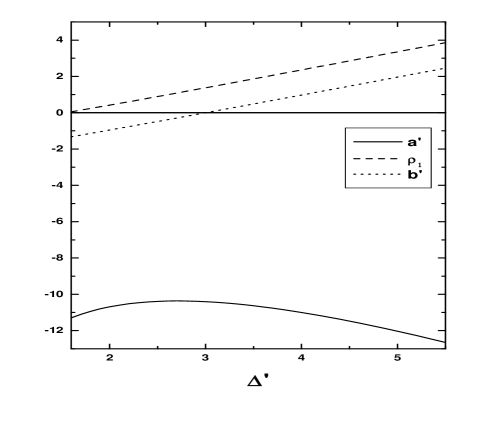
FIG. 3.: Solution of Eqs.(110-115) at temperature $T^{\prime}=20.$ The first order phase transition corresponds to the point where $b^{\prime}=0.$

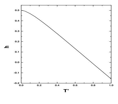
FIG. 4.: First order phase transition line at low temperatures.

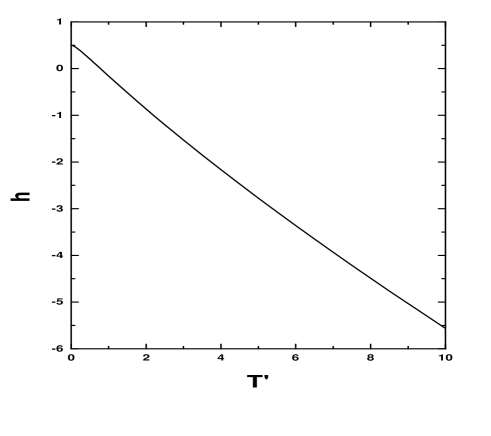
FIG. 5.: First order phase transition line.

The phase transition curve which was obtained from the above criteria is

$$a_{c}^{\prime}(T^{\prime})=h(T^{\prime}),$$ (119)

where $h$ is plotted on Figs. 4,5. The asymptotic behavior of the function $h$ at large arguments is

$$h(x)\approx-2.92\,\,x^{2/3}+2.31\,\,x^{1/2},\,\,x\gg 1,$$ (120)

with an accuracy of leading and sub-leading terms. At low temperatures the function $h(T^{\prime})$ is analytical in $T^{\prime}.$ In spite of the fact that there is a change in the kind of the transition at $T^{*},$ this curve does not have a break at this point. The phase transition line in the original notations is

$$a_{c}^{*}+\epsilon_{0}=\epsilon_{0}\kappa_{G}^{2}\,\,h\left({T\over{\epsilon_{0}\kappa_{G}^{2}}}\right),$$ (121)

where $a^{*}$ is $a$ renormalized by quantum fluctuations (24). One can see that this curve scales with the Ginzburg parameter $\kappa_{G}$.

According to the form of (121) one can define too regimes: the low-temperature, quantum regime

$$T\ll\epsilon_{0}\kappa_{G}^{2},$$ (122)

and high-temperature, classical one

$$T\gg\epsilon_{0}\kappa_{G}^{2}.$$ (123)

Note that the quantum region extends as $\kappa_{G}$ increases. Asymptotically in the classical regime from (121) one gets

$$a_{c}^{*}+\epsilon_{0}=-2.92\,\epsilon_{0}\left({{\kappa_{G}T}\over{\epsilon_{0}}}\right)^{2/3},$$ (124)

which agrees with the estimation (27).

VIII Low-energy spectrum.

In this section we will show that the low-energy spectrum of fluctuations in our model is different from one which follows from the Eilenberger theory. In our model the Eilenberger result can be obtained if one neglects the terms on the l.h.s. of Eqs.(67,69). These terms are small if we are not too close to the phase transition line, nevertheless they are always not equal to zero, and as we will show they change the low-energy spectrum considerably. If we neglect the mentioned terms in Eqs.(67,69) then we have

$$\Delta=bu,$$ (125)

$$\rho_{\bf r}=buK({\bf r}),$$ (126)

and for the lower energy branch we get

$$E_{-}({\bf r})=2bu(K({\bf r})-|Q({\bf r})|)-2bu(K(0)-|Q(0)|),$$ (127)

where we used that $E_{-}(0)=0.$ It happens that if we expand this expression in powers of ${\bf r},$ then the terms quadratic in ${\bf r}$ cancel each other and the expansion starts from $r^{4}$ term

$$E_{-}({\bf r})\sim r^{4}.$$ (128)

This result leads to divergences, for example the fluctuation contribution to the density in case $d=3$ ,$T\neq 0$ is logarithmically divergent

$$\int{{d^{2}r\,dp}\over{p^{2}+E_{-}({\bf r})}}\sim\int{{d^{2}r}\over{r^{2}}}.$$ (129)

Also the fluctuation correction to the conductivity has a logarithmic singularity [10]. The fact that there are infra-red divergences means that one needs a more careful analysis of the infra-red behavior of the model. The similar situation happens in the two-dimensional Bose gas at non zero temperatures. The Bogolubov approximation leads to the divergent fluctuation contribution to the density, but the careful analysis of the infrared behavior based on the effective low-energy functional leads to the theory without divergences. To the best of our knowledge the asymptotic behavior of the model under consideration was not found yet.

In our large-$N$ model this problem does not arise because due to the fluctuation contribution the fine tuning between the particle-hole and particle-particle parts of the spectrum ($\rho_{\bf r}$ and $\Delta|Q({\bf r}|$) does not happen, and one expects that the leading term in the low-energy spectrum is $r^{2}$

$$E_{-}({\bf r})\sim r^{2}.$$ (130)

In case of high dimensions one can see this explicitly from Eq.(83). And in general case, one can see that the particle-particle and particle-hole parts of the spectrum are affected by the fluctuation terms in a different way and therefore we do not expect any fine tuning between these terms.

We think that the result $E_{-}({\bf r})\sim r^{2}$ is specific for the large$-N$ model, and the situation in the real model is much more complicated. Nevertheless, we think that the large$-N$ model is a reasonable model for the description of the phase transition, because the infra-red properties seem to be irrelevant for the phase transition. Indeed, usually the infra-red divergences are absent in the perturbation expansion for the physical quantities like free energy, density, etc. And it is enough to know the free energy to determine the kind of the phase transition and to find the phase transition line.

IX Discussion and Conclusions.

We considered the effect of order parameter fluctuations on the transition between normal and mixed superconducting states in pure superconductors. Our starting point was an effective functional of GL type. We showed that the coefficients in this functional are finite (i.e. this functional exists) in the quasi-two-dimensional situation, when the applied magnetic field is parallel to the low-conducting direction. This case is interesting from the point of view of high$-T_{c}$ superconductors, because they have a quasi-two-dimensional band structure. We considered this functional in the large$-N$ limit. One should be careful introducing the n-index into the Lagrangian, because the symmetry between the particle-hole and particle-particle channels is very important for this problem. Indeed, introducing the n-index in the usual way

$$\phi^{*}\phi\phi^{*}\phi\to\phi^{*}_{n}\phi_{n}\phi^{*}_{m}\phi_{m},$$ (131)

in the large$-N$ limit one effectively drops out the particle-particle channel, and it leads to the model with an unstable spectrum of fluctuations. Therefore we introduce the n-index in the following way:

$$\phi^{*}\phi\phi^{*}\phi\to 2\phi^{*}_{n}\phi_{n}\phi^{*}_{m}\phi_{m}-\phi^{*}_{n}\phi_{n}^{*}\phi_{m}\phi_{m}.$$ (132)

The coefficients in the above formula can be found from the following consideration: The effect of fluctuations can be formally suppressed reducing the Ginzburg number. And in this limiting case the Eilenberger theory becomes exact. We want our large$-N$ model to be as close to the real model as possible, and therefore in the limiting case $\kappa_{G}\to 0$ we should have the Eilenberger answer for the spectrum. This requirement uniquely defines the coefficients in (132).

To simplify the large$-N$ equations we used the lowest Landau level approximation which is valid when the order parameter is much smaller than $\epsilon_{0},$ i.e. when we are not too far from the phase transition line. These large$-N$ equations can be easily solved in case of high dimensions: either $d_{\perp}>4,\,T\not=0$ or $d_{\perp}>2,\,T=0.$ In these cases the transition was found to be of the second order if the interaction constant is not too large. It is interesting to draw a parallel between our solution of the large$-N$ model and the renormalization group approach to the quantum critical phenomena problems[11, 12]. In our case the dynamical exponent $z=2.$ Note that the magnetic field “eats” two dimensions, therefore the straightforward application of the results [11, 12] gives that the upper critical dimension at zero temperature is $d_{\perp}=4-z=2,$ which agrees with our approach. The phase transition line in the large$-N$ limit was found to be

$$H_{c2}-H_{c2}^{(0)*}\sim-T^{d_{\perp}/2}\,\,,\,\,\,2<d_{\perp}<4,$$ (133)

where $H_{c2}^{(0)*}$ is the mean field upper critical field renormalized by the quantum fluctuations. In fact this result is more general than that of the large$-N$ limit. Indeed, the difference between our model and the standard GL model (which was considered in Ref.[11]) arises only when one considers the renormalization of $u$ term [5]. But in the case under consideration the $u$ term is irrelevant and therefore one should get the usual answer. Therefore the answer (133) should hold in case $N=1$ too.

In case of physical dimensionality ($d_{\perp}=1$) the model gives the first order phase transition. The fact that at finite temperatures the phase transition is of the first order looks natural because the fluctuation contribution diverges as one reaches the phase transition line from the normal state. (For example the first order correction to the “mass” term diverges as $1/\sqrt{\delta}$, see (23).) This situation is similar to one which happens in the model studied by Brazovskiy in Ref.[4], where the fluctuations drive the phase transition to the first order one. Therefore we think that in the real model at finite temperatures the transition is of the first order too. At zero temperature the large$-N$ model also gives the first order phase transition, but it is not clear whether in the real model the transition should be necessarily of the first order at zero temperature.

The phase transition line which follows from our model is

$$a_{c}^{*}+\epsilon_{0}=\epsilon_{0}\kappa_{G}^{2}\,\,h\left({T\over{\epsilon_{0}\kappa_{G}^{2}}}\right),$$ (134)

where $h$ is plotted on Figs. 4,5, and

$${{a_{c}^{*}+\epsilon_{0}}\over{\epsilon_{0}}}\sim{{H_{c2}-H_{c2}^{(0)*}}\over{H_{c2}^{(0)}}}.$$ (135)

Note that we considered only the low-temperature part of the phase diagram $T\ll\epsilon_{0},$ so that the result (135) may be applied only in this case. According to the form of (135) one can define to regimes: $T\ll\epsilon_{0}\kappa_{G}^{2}$ corresponding to the quantum fluctuations, and $T\gg\epsilon_{0}\kappa_{G}^{2}$ corresponding to the classical ones. Note that increase of the Ginzburg number makes the problem more quantum. For example if $\kappa_{G}\sim 1$, then one cannot reach the classical region because our theory works when $T\ll\epsilon_{0}.$ Asymptotically in the classical region the phase transition line is

$$a_{c}^{*}+\epsilon_{0}=-2.92\,\epsilon_{0}\left({{\kappa_{G}T}\over{\epsilon_{0}}}\right)^{2/3}.$$ (136)

Qualitatively the phase transition line looks similar to the experimental data [3] on overdoped high$-T_{c}$ materials: The upper critical field significantly increases as temperature decreases showing a nonanalytical dependence. In our theory, the curvature of the phase transition line is negative in the classical regime, but at low temperatures it becomes positive (see Fig.4). Note that the Ginzburg number in this problem is proportional to the anisotropy $\kappa_{G}\sim{{k_{a}}\over{p_{F}^{2}S}}$, that enhances the fluctuation contribution. Indeed the resistive phase transition is broad in this materials, that supports that the fluctuation contribution is large.

Finally, to avoid confusion, we note that in the high temperature superconductors, a line in the H-T plane referred to as the irreversibility line, is usually interpreted in terms of the melting of the vortex lattice. To address these experiments our work should be generalized to incorporate the effects of disorder which are beyond the scope of our paper. However, low enough disorder should not affect the melting line. Therefore in that case the transition line which was found in the paper can be considered as the irreversibility line.