Phase transition in the passive scalar advection

Abstract

The paper studies the behavior of the trajectories of fluid particles in a compressible generalization of the Kraichnan ensemble of turbulent velocities. We show that, depending on the degree of compressibility, the trajectories either explosively separate or implosively collapse. The two behaviors are shown to result in drastically different statistical properties of scalar quantities passively advected by the flow. At weak compressibility, the explosive separation of trajectories induces a familiar direct cascade of the energy of a scalar tracer with a short-distance intermittency and dissipative anomaly. At strong compressibility, the implosive collapse of trajectories leads to an inverse cascade of the tracer energy with suppressed intermittency and with the energy evacuated by large scale friction. A scalar density whose advection preserves mass exhibits in the two regimes opposite cascades of the total mass squared. We expect that the explosive separation and collapse of Lagrangian trajectories occur also in more realistic high Reynolds number velocity ensembles and that the two phenomena play a crucial role in fully developed turbulence.

PACS: 47.27 - Turbulence, fluid dynamics

1 Introduction

One of the main characteristic features of the high Reynolds number turbulent flows is a cascade-like transfer of the energy injected by an external source. In three dimensional flows, the injected energy is transferred to shorter and shorter scales and is eventually dissipated by the viscous friction. This direct cascade is in the first approximation described by the Kolmogorov 1941 scaling theory [1] but the observed departures from scaling (intermittency) remain to be explained from the first principles. As discovered by R.H. Kraichnan in [2], in two dimensions, the injected energy is transferred to longer and longer distances in an inverse cascade whereas this is the enstrophy that is transferred to shorter and shorter scales. Experiments [3] and numerical simulations [4, 5] suggest the absence of intermittency in the inverse 2-dimensional cascade. In the present paper, we shall put forward arguments indicating that the occurrence and the properties of direct and inverse cascades of conserved quantities in hydrodynamical flows are related to different typical behaviors of fluid particle trajectories.

Let us start by drawing some simple analogies between fluid dynamics and the theory of dynamical systems which studies solutions of the ordinary differential equations

$${{dx}\over{dt}}\,=\,X(x)\hskip 0.71114pt.$$ (1.1)

Let $x_{{}_{s,y}}(t)$ denote the solution of Eq.  (1.1) passing at time $s$ by point $y$. In dynamical systems, where the attention is concentrated on regular functions $X$, one encounters different types of behavior of solutions

1).  integrable motions (more common in Hamiltonian systems), where the nearby trajectories stay close together forever:

$$|x_{{}_{s,y_{1}}}(t)-\hskip 0.71114ptx_{{}_{s,y_{2}}}(t)|\ \sim\ {\cal O}(|y_{1}-y_{2}|)\hskip 0.71114pt,\ \qquad$$ (1.2)

2).  chaotic motions where the distance between the nearby trajectories grows exponentially, signaling a sensitive dependence on the initial conditions:

$$|x_{{}_{s,y_{1}}}(t)-\hskip 0.71114ptx_{{}_{s,y_{2}}}(t)|\ \sim\ {\cal O}({\rm e}^{\lambda|t-s|}|y_{1}-y_{2}|)\hskip 0.71114pt,\,$$ (1.3)

with the Lyapunov exponent $\lambda>0$ ,

3).  last but, by no means, least, dissipative motions where

$$|x_{{}_{s,y_{1}}}(t)-\hskip 0.71114ptx_{{}_{s,y_{2}}}(t)|\ \sim\ {\cal O}({\rm e}^{\lambda|t-s|}|y_{1}-y_{2}|)\hskip 0.71114pt,$$ (1.4)

with $\lambda<0$.

Various of these types of motions may appear in the same systems.

Analogies between dynamical systems and hydrodynamical evolution equations, for example the Navier Stokes ones, are often drawn by viewing the Eulerian evolution of velocities as a dynamical system in infinite dimensions, see [6]. One has, however, a more direct (although not unrelated) analogy between Eq.  (1.1) and the ordinary differential equation

$${{d{{\bf x}}}\over{dt}}\ =\ {{\bf v}}(t,{{\bf x}})$$ (1.5)

for the Lagrangian trajectories of fluid particles in a given velocity field ${{\bf v}}(t,{{\bf x}})$. As before, we shall denote by ${{\bf x}}_{{}_{s,{{\bf r}}}}(t)$ the solution passing by ${{\bf r}}$ at time $s$. Clearly, the system (1.5) is time-dependent and the velocity field is itself a dynamical variable. Nevertheless, one may ask questions about the behavior of solutions of Eq.  (1.5) for ”typical” velocities. On the phenomenological level, such behavior seems to be rather robust and to depend on few characteristics of the velocity fields. One of them is the Reynolds number $Re={L\hskip 0.71114pt|\Delta_{{}_{L}}{{\bf v}}|\over\nu}$, where $|\Delta_{{}_{L}}{{\bf v}}|$ is the (typical) velocity difference over the distance $L$ of the order of the size of the system and $\nu$ is the kinematic viscosity. Another important characteristic of velocity fields is the degree of compressibility measured, for example, by the ratio of mean values of $(\sum\limits_{\alpha}\nabla_{\alpha}v^{\alpha})^{2}\equiv(\nabla\cdot{{\bf v}})^{2}$ and $\sum\limits_{\alpha,\beta}(\nabla_{\alpha}v^{\beta})^{2}\equiv(\nabla{{\bf v}})^{2}$.

Reynolds numbers ranging up to ${\cal O}(10^{2})$ are the realm of laminar flows and the onset of turbulence. Velocity fields in (1.5) are thus regular in space and the behaviors (1) to (3) are observed for Lagrangian trajectories. They seem to have limited bearing on the character of the Eulerian evolution of velocities, see Chapter 8 of [7]. This is a natural domain of applications of the theory of dynamical systems to both Eulerian and Lagrangian evolutions. When the Reynolds number is increased, however, fully developed turbulent flows are produced in which the behavior of trajectory separations becomes more dramatic. For incompressible flows, for example, we claim (see also [8, 9, 10]) that the regime of fully developed turbulence is characterized by the

2’). explosive separation of trajectories:

$$\qquad\qquad|{{\bf x}}_{{}_{s,{{\bf r}}_{1}}}(t)-\hskip 0.71114pt{{\bf x}}_{{}_{s,{{\bf r}}_{2}}}(t)|\quad\ {\rm becomes\ }{\cal O}(1)\ {\rm in\ finite\ time}\hskip 0.71114pt.$$ (1.6)

More precisely, the time of separation of trajectories to an ${\cal O}(1)$ distance is bounded when $y_{2}$ approaches $y_{1}$, provided that the initial separation $|y_{1}-y_{2}|$ stays in the inertial range where the viscous effects may be neglected.

Since the inertial range extends down to zero distance when $Re\to\infty$, the fast separation of trajectories has a drastic consequence in this limit: the very concept of individual Lagrangian trajectories breaks down. Indeed, at $Re=\infty$, infinitesimally close trajectories take finite time to separate and, as a result, there are many trajectories (in fact, a continuum) satisfying a given initial condition. It should be still possible, however, to give a statistical description of such ensembles of trajectories in a fixed velocity field. Unlike for intermediate Reynolds numbers, there seems to be a strong relation between the behavior of the Lagrangian trajectories and the basic hydrodynamic properties of developed turbulent flows: we expect the appearance of non-unique trajectories for $Re\to\infty$ to be responsible for the dissipative anomaly, the direct energy cascade, the dissipation of higher conserved quantities and the pertinence of weak solutions of hydrodynamical equations at $Re=\infty$.

The breakdown of the Newton-Leibniz paradigm based on the uniqueness of solutions of the initial value problem for ordinary differential equations is made mathematically possible by the loss of small scale smoothness of turbulent velocities when $Re\to\infty$. At $Re=\infty$, the typical velocities are expected to be only Hölder continuous in the space variables:

$$|{{\bf v}}(t,{{\bf x}})-{{\bf v}}(t,{{\bf x}}^{\prime})|^{2}\ \sim\ |{{\bf x}}-{{\bf x}}^{\prime}|^{\xi}\hskip 0.71114pt,$$ (1.7)

with the Hölder exponent ${\xi\over 2}$ close to the Kolmogorov value ${1\over 3}$ [1]. The uniqueness of solutions of the initial value problem for Eq.  (1.5) requires, on the other hand, the Lipschitz continuity of ${{\bf v}}(t,{{\bf x}})$ in ${{\bf x}}$, i.e. the behavior (1.7) with $\xi=2$. It should be stressed that for large but finite $Re$, the chaotic behavior (2) of trajectories may still persist for short separations of the order of the dissipative scale (where the viscosity makes the velocities smooth) and the behavior (2’) is observed only on distances longer than that. However, it is the latter which seems responsible for much of the observed physics of fully developed turbulence and, thus, setting $Re=\infty$ seems to be the right idealization in this regime.

For general velocity fields, one should expect that the poor spatial regularity of velocities ${{\bf v}}$ might lead to two opposite effects. On one hand, the trajectories may branch at every time and coinciding particles would split in a finite time as in (2’). Solving discretized versions of Eq.  (1.5) randomly picks a branch of the solution and generates some sort of a random walk whose average reproduces the trajectory statistics. This is the effect previously remarked [8, 9, 10] in the studies of the incompressible Kraichnan model [11]. It should be dominant for incompressible or weakly compressible flows. On the other hand, the trajectories may tend to be trapped together. The most direct way to highlight this phenomenon is to consider strongly compressible velocity fields which are well known for depleting transport (see [12]). An instance is provided by the one-dimensional equation $\,{dx\over dt}\hskip 0.71114pt=\hskip 0.71114pt\beta(x)\hskip 0.71114pt,\,$ for $\beta(x)$ a Brownian motion in $x$, whose solutions are trapped in finite time at the zeros of $\beta$ on the right (left) ends of the intervals where $\beta>0$ ($\beta<0$) [13].

What may then become typical in strongly compressible velocities is, instead of the explosion (2’), the

3’). implosive collapse of trajectories:

$$\qquad\qquad|{{\bf x}}_{{}_{s,{{\bf r}}_{1}}}(t)-\hskip 0.71114pt{{\bf x}}_{{}_{s,{{\bf r}}_{2}}}(t)|\quad\ {\rm becomes\ equal\ to\ zero\ in\ finite\ time}\hskip 0.71114pt,$$ (1.8)

with the time of collapse depending on the initial positions. This type of behavior should lead to a domination at infinite $Re$ and strong compressibility of shock-wave-type solutions of hydrodynamical equations, as in the 1-dimensional Burgers problem [14]. Again, strictly speaking, we should expect behavior (3’) only for $Re=\infty$ whereas for finite $Re$, on distances smaller than the dissipative scale, the approach of typical trajectories should become exponential with a negative Lyapunov exponent. In simple Gaussian ensembles of smooth compressible velocities the latter behavior and its consequences for the direction of the cascade of a conserved quantity have been discovered and extensively discussed in [15] and [16].

It is the main purpose of the present paper to provide some support for the above, largely conjectural, statements about typical behaviors of fluid-particle trajectories at high Reynolds numbers and about the impact of these behaviors on physics of the fully turbulent hydrodynamical flows. We study only simple synthetic random ensembles of velocities showing Hölder continuity in spatial variables. Although this is certainly insufficient to make firm general statements, it shows, however, that the behaviors (2’) and (3’) are indeed possible and strongly affect hydrodynamical properties. In realistic flows, both behaviors might coexist. For the ensemble of flows considered here, they occur alternatively, leading to two different phases at large (infinite) Reynolds numbers, depending on the degree of compressibility and the space dimension. The occurrence of the collapse (3’) is reflected in the suppression of the short-scale dissipation and the inverse cascade of certain conserved quantities. The absence of dissipative anomaly permits an analytical understanding of the dynamics and to show that the inverse cascade is self-similar. This strengthens the conjectures on the general lack of intermittency for inverse cascades [3, 4, 5, 17]. A caveat comes however from the consideration of friction effects, indicating that the role of infrared cutoffs might be subtle and anomalies might reappear in terms of them.

Synthetic ensembles of velocities are often used to study the problems of advection in hydrodynamical flows. These problems become then simpler to understand than the advection in the Navier-Stokes flows, but might still render well some physics of the latter, especially in the case of passive advection when the advected quantities do not modify the flows in an important way. The simplest of the problems concern the advection of scalar quantities. There are two types of such quantities that one may consider. The first one, which we shall call a tracer and shall denote $\theta(t,{{\bf r}})$, undergoes the evolution governed by the equation

$$\partial_{t}\theta+{{\bf v}}\cdot\nabla\theta-\kappa\nabla^{2}\theta=f\hskip 0.71114pt,$$ (1.9)

where $\kappa$ denotes the diffusivity and $f(t,{{\bf r}})$ describes an external forcing (a source). The second scalar quantity is of a density type, e.g. the density of a pollutant, and we shall denote it by $\rho(t,{{\bf r}})$. Its evolution equation is

$$\partial_{t}\rho+\nabla\cdot({{\bf v}}\hskip 0.71114pt\rho)-\kappa\nabla^{2}\rho=f\hskip 0.71114pt.$$ (1.10)

For $f=0$ it has a form of the continuity equation so that, without the source, the evolution of $\rho$ preserves the total mass $\int\rho(t,{{\bf r}})\hskip 0.71114ptd{{\bf r}}$. Both equations coincide for incompressible velocities but are different if the velocities are compressible.

A lot of attention has been attracted recently by a theoretical and numerical study of a model of the passive scalar advection introduced by R. H. Kraichnan in 1968 [18]. The essence of the Kraichnan model is that it considers a synthetic Gaussian ensemble of velocities decorrelated in time. The ensemble may be defined by specifying the 1-point and the 2-point functions of velocities. Following Kraichnan, we assume that the mean velocity $\langle\hskip 0.71114pt{{\bf v}}(t,{{\bf x}})\hskip 0.71114pt\rangle$ vanishes and that

$$\langle v^{\alpha}(t,{{\bf r}})\,v^{\beta}(t^{\prime},{{\bf r}}^{\prime})\rangle=\delta(t-t^{\prime})\,[\hskip 0.71114ptd_{0}^{\alpha\beta}-d^{\alpha\beta}({{\bf r}}-{{\bf r}}^{\prime})\hskip 0.71114pt]$$ (1.11)

with constant $d_{0}^{\alpha\beta}$ and with $d^{\alpha\beta}({{\bf r}})$ proportional to $r^{\xi}$ at short distances. The latter property mimics the scaling behavior of the equal-time velocity correlators of realistic turbulent flows in the $Re\to\infty$ limit. It leads to the behavior (1.7) for the typical realizations of ${{\bf v}}$. The parameter $\xi$ is taken between $0$ and $2$ so that the typical velocities of the ensemble are not Lipschitz continuous.

We shall study the behavior of Lagrangian trajectories in the velocity fields of a compressible version of the Kraichnan ensemble and the effect of that behavior on the advection of the scalars. The time decorrelation of the velocity ensemble is not a very physical assumption. It makes, however, an analytic study of the model much easier. We expect the temporal behavior of the velocities to have less bearing on the behavior of Lagrangian trajectories than the spatial one, but this might be the weakest point of our arguments. Another related weak point is that the Kraichnan ensemble is time-reversal invariant whereas realistic velocity ensembles are not, so that the typical behaviors of the forward- and backward-in-time solutions of Eq.  (1.5) for the Lagrangian trajectories may be different. It should be also mentioned that in our conclusions about the advection of scalars we let $Re\to\infty$ before sending the diffusivity $\kappa$ to zero, i.e. we work at zero Schmidt or Prandtl number $\nu\over\kappa$. The qualitative picture should not be changed, however, if $Re$ becomes very large but $\nu\over\kappa$ stays bounded. On the other hand, the situation when ${\nu\over\kappa}\to\infty$ should be better described by the $\xi\to 2$ limit of the Kraichnan model where the velocities become smooth.

The paper is organized as follows. In Sect.  2 we discuss the statistics of the Lagrangian trajectories in the Kraichnan ensemble and discover two different phases with typical behaviors (2’) and (3’), occurring, respectively, in the case of weak and strong compressibility. In Sects.  3 and 4 we discuss the advection of a scalar tracer in both phases and show that it exhibits cascades of the mean tracer energy. In the weakly compressible phase, the cascade is direct (i.e. towards short distances) and it is characterized by an intermittent behavior of tracer correlations, signaled by their anomalous scaling at short distances. On the other hand, in the strongly compressible phase, the tracer energy cascade inverts its direction. In the latter case, we compute exactly the probability distribution functions of the tracer differences over long distances and show that, although non-Gaussian, they have a scale-invariant form. This indicates that the inverse cascade directed towards long distances forgets the integral scale where the energy is injected. Conversely, the scale where friction extracts energy from the system is shown in Section 6 to lead to anomalous scaling of certain observables. Finally, in Section 7, we discuss briefly the advection of a scalar density. Here, in the weakly compressible phase, we find a cascade of the mean mass squared towards long distances and, on short distances, the scaling of correlation functions in agreement with the predictions of [19]. The strongly compressible shock-wave phase, however, exhibits a drastically different behavior with the inversion of the direction of the cascade of mean mass squared towards short distances. In Conclusions we briefly summarize our results. Some of the more technical material is assembled in five Appendices.

2 Lagrangian flow

The assumptions of isotropy and of scaling behavior on all scales fix the functions $d^{\alpha\beta}(x)$ in the velocity 2-point function (1.11) of the Kraichnan ensemble up to two parameters:

$$d^{\alpha\beta}({{\bf r}})=[A+(d+\xi-1)B]\,\delta^{\alpha\beta}\hskip 0.71114ptr^{\xi}\,+\,[A-B]\,\xi\hskip 0.71114ptr^{\alpha}r^{\beta}\hskip 0.71114ptr^{\xi-2}\hskip 0.71114pt,$$ (2.1)

with $A=0$ corresponding to the incompressible case where $\nabla\cdot{{\bf v}}=0$ and $B=0$ to the purely potential one with ${{\bf v}}=\nabla\phi$. Positivity of the covariance requires that $A,B\geq 0$. It will be convenient to relabel the constants $A$ and $B$ by ${\cal S}^{2}=A+(d-1)B$ and ${\cal C}^{2}=A$. ${\cal S}^{2}$ and ${\cal C}^{2}$ are proportional to, respectively, $\langle(\nabla{{\bf v}})^{2}\rangle$ and $\langle(\nabla\cdot{{\bf v}})^{2}\rangle$ and they satisfy the inequalities ${\cal S}^{2}\geq{\cal C}^{2}\geq 0$. In one dimension, ${\cal S}^{2}={\cal C}^{2}\geq 0$. The ratio

$$\wp\equiv{{\cal C}^{2}\over{\cal S}^{2}},\quad 0\leq\wp\leq 1,$$ (2.2)

characterizes the degree of compressibility.

The source $f$ in the evolution equations (1.9) and (1.10) for the scalars will be also taken random Gaussian, independent of velocity, with mean zero and 2-point function

$$\langle f(t,{{\bf r}})\,f(t^{\prime},{{\bf r}}^{\prime})\rangle=\delta(t-t^{\prime})\,\chi({|{{\bf r}}-{{{\bf r}}}^{\prime}|})\hskip 0.71114pt,$$ (2.3)

where $\chi$ decays on the injection scale $L$.

In the absence of the forcing and diffusion terms in Eq.  (1.9), the tracer $\theta$ is carried by the flow: $\theta(t,{{\bf r}})\,=\,\theta(s,{{\bf x}}_{{}_{t,{{\bf r}}}}(s))$, and the density $\rho$ is stretched as the Jacobian $J={\partial({{\bf x}}_{t,{{\bf r}}}(s))}/{\partial({{\bf r}})}$ of the map ${{\bf r}}\mapsto{{\bf x}}_{t,{{\bf r}}}(s)$: $\rho(t,{{\bf r}})\,=\,\rho(s,{{\bf x}}_{{}_{t,{{\bf r}}}}(s))\,J$. Here, ${{\bf x}}_{t,{{\bf r}}}(s)$ is the fluid (Lagrangian) trajectory obeying $d{{\bf x}}_{{}_{t,{{\bf r}}}}/ds=v(s,{{\bf x}}_{{}_{t,{{\bf r}}}})$ and passing through the point ${{\bf r}}$ at time $t$, i.e. ${{\bf x}}_{{}_{t,{{\bf r}}}}(t)={{\bf r}}$. The flows of the scalars may be rewritten as the relations

$$\theta(t,{{\bf r}})=\int\delta({{\bf r}}^{\prime}-{{\bf x}}_{{}_{t,{\bf r}}}(s))\,\theta(s,{{\bf r}}^{\prime})\,\hskip 0.71114ptd{{\bf r}}^{\prime}\hskip 0.71114pt,\qquad\rho(t,{{\bf r}})=\int\delta({{\bf r}}-{{\bf x}}_{{}_{s,{\bf r}^{\prime}}}(t))\,\rho(s,{{\bf r}}^{\prime})\,\hskip 0.71114ptd{{\bf r}}^{\prime}\quad$$ (2.4)

which imply that the two flows are dual to each other: $\,\int\theta(t,{{\bf r}})\,\rho(t,{{\bf r}})\,d{{\bf r}}$ does not change in time. In the presence of forcing and diffusion, there are some slight modifications. First, the sources create the scalars along the Lagrangian trajectories. Second, the diffusion superposes Brownian motions upon the trajectories. One has

$$\theta(t,{{\bf r}})\ =\ \overline{\theta(s,{{\bf x}}_{{}_{t,{{\bf r}}}}(s))\hskip 0.71114pt+\hskip 0.71114pt\smallint\limits_{s}^{t}f(\tau,{{\bf x}}_{{}_{t,{{\bf r}}}}(\tau))\,d\tau}$$ (2.5)

for the tracer and

$$\rho(t,{{\bf r}}) = \overline{\rho(s,{{\bf x}}_{{}_{t,{{\bf r}}}}(s))\,{{}_{\partial({{\bf x}}_{t,{{\bf r}}}(s))}\over{}^{\partial({{\bf r}})}}\hskip 0.71114pt+\hskip 0.71114pt\smallint\limits_{s}^{t}f(\tau,{{\bf x}}_{{}_{t,{{\bf r}}}}(\tau))\,{{}_{\partial({{\bf x}}_{t,{{\bf r}}}(\tau))}\over{}^{\partial({{\bf r}})}}\,d\tau}$$ (2.6)

for the density, where

$${d{{\bf x}}_{{}_{t,{{\bf r}}}}\over ds}=v(s,{{\bf x}}_{{}_{t,{{\bf r}}}})\hskip 0.71114pt+\hskip 0.71114pt\sqrt{2\kappa}\,{d{\bf{\beta}}\over ds}\hskip 0.71114pt,\qquad{{\bf x}}_{{}_{t,{{\bf r}}}}(t)={{\bf r}}\hskip 0.71114pt,$$ (2.7)

with the overbar in Eqs.  (2.5) and (2.6) denoting the average over the $d$-dimensional Brownian motions ${\bf{\beta}}(s)$.

Clearly, the statistics of the scalar fields reflects the statistics of the Lagrangian trajectories or, for $\kappa>0$, of their perturbations by the Brownian motions. In particular, it will be important to look at the probability distribution functions (p.d.f.’s) of the difference ${{\bf r}}^{\prime}$ of time $s$ positions of two Lagrangian trajectories (perturbed by independent Brownian motions if $\kappa>0$), given their time $t$ positions ${{\bf r}}_{1}$ and ${{\bf r}}_{2}$,

$$P_{2}^{t,s}({{\bf r}}_{1}-{{\bf r}}_{2},\hskip 0.71114pt{{\bf r}}^{\prime})\,=\,\langle\,\delta({{\bf r}}^{\prime}-{{\bf x}}_{{}_{t,{{\bf r}}_{1}}}(s)+{{\bf x}}_{{}_{t,{{\bf r}}_{2}}}(s))\,\rangle\hskip 0.71114pt.$$ (2.8)

Note that $P_{2}^{t,s}$ is normalized to unity with respect to ${{\bf r}}^{\prime}$ and the equivalent expressions

$$P_{2}^{t,s}({{\bf r}}_{1}-{{\bf r}}_{2},\hskip 0.71114pt{{\bf r}}^{\prime}) = \int\langle\,\delta({{\bf r}}^{\prime}+{{\bf r}}-{{\bf x}}_{{}_{t,{\bf r}_{1}}}(s))\,\,\delta({{\bf r}}-{{\bf x}}_{{}_{t,{\bf r}_{2}}}(s))\,\rangle\,\,d{{\bf r}}$$ (2.9)

$$= \int\langle\,\delta({{\bf r}}^{\prime}-{{\bf x}}_{{}_{t,{\bf r}_{1}-{\bf r}}}(s))\,\,\delta(-{{\bf x}}_{{}_{t,{\bf r}_{2}-{\bf r}}}(s))\,\rangle\,\,d{{\bf r}}\hskip 0.71114pt,$$ (2.10)

where the last equality uses the homogeneity of the velocities.

In the Kraichnan model, the p.d.f.’s $P_{2}^{t,s}$ may be easily computed. They are given by the heat kernels ${\rm e}^{-|t-s|\hskip 0.71114ptM_{2}^{\kappa}}({{\bf r}},\hskip 0.71114pt{{\bf r}}^{\prime})$ of the $2^{\rm nd}$-order elliptic differential operators $M_{2}^{\kappa}\,=\,-\hskip 0.71114ptd^{\alpha\beta}({{\bf r}})\hskip 0.71114pt\nabla_{\alpha}\nabla_{\beta}\,-\,2\kappa\nabla^{2}$. What this means is that the Lagrangian trajectories undergo, in their relative motion, an effective diffusion with the generator $M_{2}^{\kappa}$, i.e. with a space-dependent diffusion coefficient proportional to their relative distance to power $\xi$ (for distances large enough that the contribution of the $\kappa$-term to $M_{2}^{\kappa}$ may be neglected). Note that, due to the stationarity and the time reflection symmetry of the velocity distribution,

$$P_{2}^{t,s}({{\bf r}},\hskip 0.71114pt{{\bf r}}^{\prime})\,=\,P_{2}^{s,t}({{\bf r}},\hskip 0.71114pt{{\bf r}}^{\prime})$$ (2.11)

but that, in general, $P_{2}^{t,s}({{\bf r}},\hskip 0.71114pt{{\bf r}}^{\prime})\not=P_{2}^{s,t}({{\bf r}}^{\prime},\hskip 0.71114pt{{\bf r}})$, except for the incompressible case where the operator $M_{2}^{\kappa}$ becomes symmetric.

2.1 Statistics of inter-trajectory distances

For many purposes, it will be enough to keep track only of the distances between two Lagrangian trajectories. We shall then restrict the p.d.f.’s $P_{2}^{t,s}$ to the isotropic sector by defining

$$P_{2}^{t,s}(r,r^{\prime})\,=\,\int\limits_{SO(d)}P_{2}^{t,s}(\Lambda{{\bf r}},\hskip 0.71114pt{{\bf r}}^{\prime})\,\hskip 0.71114ptd\Lambda\,=\,\,\int\limits_{SO(d)}P_{2}^{t,s}({{\bf r}},\hskip 0.71114pt\Lambda{{\bf r}}^{\prime})\,\hskip 0.71114ptd\Lambda\hskip 0.71114pt,$$ (2.12)

where $d\Lambda$ stands for the normalized Haar measure on $SO(d)$. $P_{2}^{t,s}(r,r^{\prime})$ is the p.d.f. of the time $s$ distance $r^{\prime}$ between two Lagrangian trajectories, given their time $t$ distance $r$. Clearly,

$$P_{2}^{t,s}(r,r^{\prime})\ =\ {\rm e}^{-|t-s|\hskip 0.71114ptM_{2}^{\kappa}}(r,r^{\prime})$$ (2.13)

with the operator $M_{2}^{\kappa}$ restricted to the isotropic sector. In the action on rotationally invariant functions,

$$M_{2}^{\kappa}\,=\,-\hskip 0.71114ptZ\hskip 0.71114ptr^{\xi-a}\partial_{r}r^{a}\partial_{r}\,-\,2\kappa\,r^{-d+1}\partial_{r}r^{d-1}\partial_{r}\hskip 0.71114pt,$$ (2.14)

where

$$Z\hskip 0.71114pt=\hskip 0.71114pt{\cal S}^{2}+\xi\hskip 0.71114pt{\cal C}^{2}\qquad{\rm and}\qquad a\,=\,[(d-1+\xi)\hskip 0.71114pt{\cal S}^{2}-\xi\hskip 0.71114pt{\cal C}^{2}]\hskip 0.71114ptZ^{-1}\hskip 0.71114pt.$$ (2.15)

The radial Laplacian which constitutes the $\kappa$-term of $M_{2}^{\kappa}$ should be taken with the Neumann boundary conditions at $r=0$ since the smooth rotationally invariant functions on ${{\bf R}}^{d}$ satisfy $\partial_{r}f(0)=0$. This is the term that dominates at small $r$ and, consequently, we should choose the same boundary condition for the complete operator $M_{2}^{\kappa}$. The adjoint operator $(M_{2}^{\kappa})^{*}$ with respect to the $L^{2}$ scalar product $\|f\|^{2}=\smallint\limits_{0}^{\infty}|f(r)|^{2}d\mu_{d}(r)$, where $d\mu_{d}(r)=S_{d-1}\hskip 0.71114ptr^{d-1}\hskip 0.71114ptdr$ with $S_{d-1}$ standing for the volume of the unit sphere in $d$-dimensions, should be taken with the adjoint boundary conditions which make the integration by parts possible. The diagonalization of $M_{2}^{\kappa}$ (in the isotropic sector), if possible, would then permit to write

$$P_{2}^{t,s}(r,r^{\prime})\,=\,\int{\rm e}^{-|t-s|\hskip 0.71114ptE}\,\phi_{E}(r)\,\psi_{E}(r^{\prime})\,\hskip 0.71114ptd\nu(E)\hskip 0.71114pt,$$ (2.16)

where $\phi_{E}$ and $\psi_{E}$ stand for the eigen-functions of the operators $M_{2}^{\kappa}$ and $(M^{\kappa}_{2})^{*}$, respectively, and $d\nu(E)$ for the spectral measure. We could naively expect that the same picture remains true for $\kappa=0$ when

$$M_{2}\,\equiv\,M_{2}^{0}\,=\,-Z\hskip 0.71114ptr^{\xi-a}\partial_{r}r^{a}\partial_{r}$$ (2.17)

in the rotationally invariant sector. The problem is that the principal symbol of the operator $M_{2}$ vanishes at $r=0$ so that the operator looses ellipticity there and more care is required in the treatment of the boundary condition.

We start by a mathematical treatment of the problem whose physics we shall discuss later. It will be convenient to introduce the new variable $u=r^{2-\xi\over 2}$ and to perform the transformation

$$(Uf)(u)\,=\,({{}_{2\hskip 0.71114ptS_{d-1}}\over{}^{2-\xi}})^{{}^{1\over 2}}\,u^{{d\over 2-\xi}-{1\over 2}}\,f(u^{2\over 2-\xi})$$ (2.18)

mapping unitarily the space of square integrable rotationally invariant functions on ${{\bf R}}^{d}$ to $L^{2}({{\bf R}}_{+},du)$. The transformation $U$, together with a conjugation by a multiplication operator, turns $M_{2}$ into the well known Schrödinger operator on the half-line:

$$N_{2}\,\equiv\,u^{-c}\,U\,M_{2}\,U^{-1}\hskip 0.71114ptu^{c}\,=\,{Z^{\prime}}\,\hskip 0.71114pt[\hskip 0.71114pt-\partial_{u}^{2}\,+\,{{}_{b^{2}-{{}_{1}\over{}^{4}}}\over{}^{u^{2}}}\hskip 0.71114pt]\hskip 0.71114pt,$$ (2.19)

where

$$Z^{\prime}\,=\,{{}_{(2-\xi)^{2}}\over{}^{4}}\,Z\hskip 0.71114pt,\qquad b\,=\,{{}_{1-a}\over{}^{2-\xi}}\qquad{\rm and}\qquad c\,=\,b+{{}_{d}\over{}^{2-\xi}}-1\hskip 0.71114pt.$$ (2.20)

$N_{2}$ becomes a positive self-adjoint operator in $L^{2}({{\bf R}}_{+})$ if we specify appropriately the boundary conditions at $u=0$. The theory of such boundary conditions is a piece of rigorous mathematics [20]. It says that for $|b|<1$ there is a one-parameter family of choices of such conditions, among them two leading to the operators $N_{2}^{\mp}$ with the (generalized) eigen-functions

$$\varphi^{\mp}_{E}(u)\,=\,u^{{{}_{1}\over{}^{2}}}\,J_{\mp{b}}(\sqrt{E/Z^{\prime}}\,u)$$ (2.21)

(for $b\not=0$) behaving at $u=0$ as ${\cal O}(u^{{{}_{1}\over{}^{2}}\mp b})$, respectively. We then obtain, fixing the spectral measure by the dimensional consideration and e.g. the action of $N_{2}^{\mp}$ on functions $u^{\mu}$,

$${\rm e}^{-|t-s|\hskip 0.71114ptN^{\mp}_{2}}(u,u^{\prime})\,=\,{{}_{1}\over{}^{2\hskip 0.71114ptZ^{\prime}}}\int\limits_{0}^{\infty}{\rm e}^{-|t-s|\hskip 0.71114ptE}\,\varphi^{\mp}_{E}(u)\,\hskip 0.71114pt\varphi^{\mp}_{E}(u^{\prime})\,\,dE\hskip 0.71114pt.$$ (2.22)

Note that the flip of the sign of $b$ exchanges $N_{2}^{-}$ and $N_{2}^{+}$. Relating the operators $N_{2}^{\mp}$ to $M_{2}^{\mp}$ by Eq.  (2.19), we infer that

$${\rm e}^{-|t-s|\hskip 0.71114ptM_{2}^{\mp}}(r,r^{\prime})\hskip 0.71114pt=\hskip 0.71114pt{{}_{1}\over{}^{2\hskip 0.71114ptZ^{\prime}}}\int\limits_{0}^{\infty}{\rm e}^{-|t-s|\hskip 0.71114ptE}\,\hskip 0.71114ptU^{-1}(u^{c}\varphi^{\mp}_{E})(r)\,\hskip 0.71114ptU^{-1}(u^{-c}\varphi^{\mp}_{E})(r^{\prime})\,\hskip 0.71114ptdE$$ (2.23)

$$=\,{{}_{1}\over{}^{(2-\xi)\hskip 0.71114ptZ\hskip 0.71114ptS_{d-1}}}\int\limits_{0}^{\infty}{\rm e}^{-|t-s|\hskip 0.71114ptE}\,\,r^{1-a\over 2}\,\,J_{\mp{b}}(\sqrt{E/Z^{\prime}}\,{r^{2-\xi\over 2}})\,\hskip 34.14322pt$$ (2.24)

$$\cdot\,\,J_{\mp{b}}(\sqrt{E/Z^{\prime}}\,{{r^{\prime}}^{2-\xi\over 2}})\,\,{r^{\prime}}^{-d+{3\over 2}+{a\over 2}-\xi}\,\,dE\hskip 0.71114pt.\hskip 34.14322pt$$ (2.25)

These are explicit versions of the eigen-function expansion (2.16) for $\kappa=0$.

The eigen-functions of $M_{2}^{\mp}$ can be read of from the above formula. They behave, respectively, as ${\cal O}(1)$ and ${\cal O}(r^{1-a})$ at $r=0$. This is the first choice that corresponds to the $\kappa\to 0$ limit of the Neumann boundary condition for the operator $M_{2}^{\kappa}$. In Appendix A, we analyze a simpler problem, where the operator (2.14) is replaced by its $\kappa=0$ version (2.17) made regular by considering it on the interval $[r_{0},\infty[$, with the Neumann boundary condition at $r_{0}>0$. We show that, for $|b|<1$, this is the operator $M_{2}^{-}$ that emerges then in the limit $r_{0}\searrow 0$. The cutting of the interval at a non-zero value has a similar effect as the addition of the $\kappa$-term to $M_{2}$. We should then have the relation

$$P_{2}^{t,s}(r,r^{\prime})\,=\,{\rm e}^{-|t-s|\hskip 0.71114ptM_{2}^{-}}(r,r^{\prime})$$ (2.26)

in the $\kappa\to 0$ limit, as long as $|b|<1$.

For $|b|\geq 1$, there is only one way to make $N_{2}$ into a positive self-adjoint operator. If $b\leq-1$, it is still the operator $N_{2}^{-}$ that survives and the relation (2.26) still holds in the $\kappa\to 0$ limit. For $b\geq 1$, however, i.e. for the compressibility degree $\wp\geq{d\over\xi^{2}}$, only the operator $N_{2}^{+}$ survives. Its eigen-functions $\varphi^{+}_{E}$ behave as ${\cal O}(u^{b+{{}_{1}\over{}^{2}}})$ at $u=0$ which corresponds to the ${\cal O}(r^{1-a})$ behavior of the eigen-functions of $M_{2}^{+}$. If we impose the Neumann boundary condition for $M_{2}$ at $r=r_{0}$ then, as we show in Appendix A, in the limit $r_{0}\searrow 0$, the eigen-functions will still become proportional to the ones obtained from $\varphi^{+}_{E}$, not to those corresponding to $\varphi^{-}_{E}$ as it happens for $b<1$. The same effect has to occur if we add and then turn off the diffusivity $\kappa$. It seems then that the equality $P_{2}^{t,s}(r,r^{\prime})\,=\,{\rm e}^{-|t-s|\hskip 0.71114ptM_{2}^{+}}(r,r^{\prime})$ has to hold in the $\kappa\to 0$ limit when $b\geq 1$.

There is, however, one catch. A direct calculation, see Eqs.  (B.2) and (B.4) of Appendix B, shows that the expression (2.26) is normalized to unity with respect to $r^{\prime}$, but that

$$\int\limits_{0}^{\infty}{\rm e}^{-|t-s|\hskip 0.71114ptM_{2}^{+}}(r,r^{\prime})\,\,d\mu_{d}({r^{\prime}})\,=\,\gamma({b},\hskip 0.71114pt{{}_{r^{2-\xi}}\over{}^{4\hskip 0.71114ptZ^{\prime}\hskip 0.71114pt|t-s|}})\,\,\Gamma({b})^{{}^{-1}}\ <\ 1\hskip 0.71114pt,$$ (2.27)

where $\gamma(b,x)=\smallint\limits_{0}^{x}y^{b-1}\hskip 0.71114pt{\rm e}^{-y}\hskip 0.71114ptdy={x^{b}\over b}\,\hskip 0.71114pt{}_{{}_{1}}F_{{}_{1}}(b,1+b;-x)$ is the incomplete gamma-function. An alternative, but more instructive, way to reach the same conclusion is to observe that the time derivative of ${\rm e}^{-t\hskip 0.71114ptM_{2}^{\mp}}(r,r^{\prime})$ brings down the adjoint of $M_{2}^{\mp}$ acting on the $r^{\prime}$ variable so that

$${{}_{d}\over{}^{dt}}\,\hskip 0.71114pt\int\limits_{0}^{\infty}{\rm e}^{-t\hskip 0.71114ptM_{2}^{\mp}}(r,r^{\prime})\,\,{r^{\prime}}^{d-1}\hskip 0.71114ptdr^{\prime} = Z\int\limits_{0}^{\infty}\partial_{r^{\prime}}\hskip 0.71114pt{r^{\prime}}^{a}\partial_{r^{\prime}}\hskip 0.71114pt{r^{\prime}}^{d-1-a+\xi}\left({\rm e}^{-t\hskip 0.71114ptM_{2}^{\mp}}(r,r^{\prime})\right)$$ (2.28)

$$= Z\,{r^{\prime}}^{a}\partial_{r^{\prime}}\hskip 0.71114pt{r^{\prime}}^{d-1-a+\xi}\left({\rm e}^{-t\hskip 0.71114ptM_{2}^{\mp}}(r,r^{\prime})\right)\bigg{|}^{{}_{r^{\prime}=\infty}}_{{}^{r^{\prime}=0}}\hskip 0.71114pt.$$ (2.29)

The contribution from $r^{\prime}=\infty$ vanishes. On the other hand, $\,{\rm e}^{-t\hskip 0.71114ptM_{2}^{-}}(r,r^{\prime})\propto{r^{\prime}}^{-d+1+a-\xi}$ for small $r^{\prime}$ whereas $\,{\rm e}^{-t\hskip 0.71114ptM_{2}^{+}}(r,r^{\prime})\propto{r^{\prime}}^{-d+2-\xi}\hskip 0.71114pt$,  with the errors suppressed by an additional factor ${r^{\prime}}^{2-\xi}$. It follows that the contribution from $r^{\prime}=0$ is zero for $M_{2}^{-}$ if $1+a-\xi>0$, which is the same condition as $b<1$ or $\wp<{d\over\xi^{2}}$, but it is finite for $M_{2}^{+}$.

The lack of normalization may seem strange since when we add the diffusivity $\kappa$ and fix the Neumann boundary conditions then, by a similar argument as for $M_{2}^{-}$ above, the normalization is assured. The solution of the paradox is that for $b\geq 1$, the $\kappa\to 0$ convergence of ${\rm e}^{-t\hskip 0.71114ptM_{2}^{\kappa}}(r,r^{\prime})$ to ${\rm e}^{-t\hskip 0.71114ptM_{2}^{+}}(r,r^{\prime})$ holds only for $r^{\prime}\not=0$ and the defect of probability concentrates at $r^{\prime}=0$. For $\kappa=0$, we should then add to ${\rm e}^{-t\hskip 0.71114ptM_{2}^{+}}(r,r^{\prime})$ a delta-function term carrying the missing probability.

We infer this way that

$$\lim\limits_{\kappa\to 0}\ P^{t,s}_{2}(r,r^{\prime})\ =\ \cases{\hbox to224.7766pt{${\rm e}^{-|t-s|\hskip 0.71114ptM^{-}_{2}}(r,r^{\prime})$\hfill}{\rm for}\quad\wp<{d\over\xi^{2}}\hskip 0.71114pt,\cr\cr{\rm e}^{-|t-s|\hskip 0.71114ptM^{+}_{2}}(r,r^{\prime})\ +\ [\hskip 0.71114pt1\,-\,\gamma({b},\hskip 0.71114pt{{}_{r^{2-\xi}}\over{}^{4\hskip 0.71114ptZ^{\prime}\hskip 0.71114pt|t-s|}})\,\,\Gamma({b})^{{}^{-1}}]\,\hskip 0.71114pt\delta({{\bf r}}^{\prime})\cr\hbox to224.7766pt{{}\hfill}{\rm for}\quad\wp\geq{d\over\xi^{2}}\hskip 0.71114pt.}$$ (2.30)

In the both cases, the p.d.f.’s $P_{2}^{t,s}$ satisfy the evolution equation

$$\partial_{t}\,P_{2}^{t,s}(r,r^{\prime})\ =\ \mp\hskip 0.71114ptM_{2}\,P_{2}^{t,s}(r,r^{\prime})$$ (2.31)

where $M_{2}$, given by Eq.  (2.17), acts on the $r$-variable and the sign $\mp$ corresponds to $t{{}_{>}\atop{}^{<}}s$. They also have the composition property:

$$\int\limits_{0}^{\infty}P_{2}^{t,t^{\prime}}(r,r^{\prime})\,\hskip 0.71114ptP_{2}^{t^{\prime},t^{\prime\prime}}(r^{\prime},r^{\prime\prime})\hskip 0.71114pt\,d\mu_{d}(r^{\prime})\ =\ P_{2}^{t,t^{\prime\prime}}(r,r^{\prime\prime})$$

if $t<t^{\prime}<t^{\prime\prime}$ or $t>t^{\prime}>t^{\prime\prime}$.

It is instructive to note the long time behavior of the averaged powers of the distance between the Lagrangian trajectories. As follows from Eqs.  (B.2) and (B.4) of Appendix B, for $\mu>0$,

$$\int\limits_{0}^{\infty}P^{t,s}_{2}(r,r^{\prime})\,\,{r^{\prime}}^{\mu}\,d\mu_{d}({r^{\prime}})\ \ \sim\ \ \cases{\hbox to88.2037pt{$|t-s|^{{}^{\mu\over 2-\xi}}$ \hfill}\qquad{\rm for}\quad\wp<{d\over\xi^{2}}\hskip 0.71114pt,\cr\hbox to88.2037pt{$|t-s|^{{}^{{\mu\over 2-\xi}-b}}\,r^{1-a}$\hfill}\qquad{\rm for}\quad\wp\geq{d\over\xi^{2}}\hskip 0.71114pt.}\quad$$ (2.32)

2.2 Fully developed turbulence versus chaos

The two cases $\wp<{d\over\xi^{2}}$ and $\wp\geq{d\over\xi^{2}}$ correspond to two physically very different regimes of the Kraichnan model. Let us first notice a completely different typical behavior of Lagrangian trajectories in the two cases. In the regime $\wp<{d\over\xi^{2}}$, which includes the incompressible case ${\cal C}^{2}=0$ studied extensively before, see [10] and the references therein, the p.d.f.’s $P_{2}^{t,s}(r,r^{\prime})$ possess a non-singular limit:

$$\lim\limits_{r\to 0}\,\,P_{2}^{t,s}(r,r^{\prime})\,=\,{{}_{2-\xi}\over{}^{S_{d-1}\hskip 0.71114pt\Gamma(1-{b})\,\,(4\hskip 0.71114ptZ^{\prime}\hskip 0.71114pt|t-s|)^{1-{b}}}}\,\,r^{\prime-d+1+a-\xi}\,\,{\rm e}^{-{{r^{\prime}}^{2-\xi}\over 4\hskip 0.71114ptZ^{\prime}\hskip 0.71114pt|t-s|}}\hskip 0.71114pt.$$ (2.33)

It follows that, when the time $t$ distance of the Lagrangian trajectories tends to zero, the probability to find a non-zero distance between the trajectories at time $s\not=t$ stays equal to unity: infinitesimally close trajectories separate in finite time. This signals the ”fuzzyness” of the Lagrangian trajectories [8, 10] forming a stochastic Markov process already in a fixed typical realization of the velocity field, with the transition probabilities of the process propagating weak solutions of the passive scalar equation $\partial_{t}\theta+{{\bf v}}\cdot\nabla\theta=0$ [21]. Such appearance of stochasticity at the fundamental level seems to be an essential characteristic of fully developed turbulence in the incompressible or weakly compressible fluids. It is due to the roughness of typical turbulent velocities which are only Hölder continuous with exponent ${\xi\over 2}<1$ (in the limit of infinite Rynolds number $Re$). One should stress an important difference between this type of stochasticity and the stochasticity of chaotic behaviors. In chaotic systems, the trajectories are uniquely determined by the initial conditions but depend sensitively on the latter. The nearby trajectories separate exponentially in time at the rate given by a positive Lyapunov exponent. The exponential separation implies, however, that infinitesimally close trajectories take infinite time to separate. This type of behavior is observed in flows with intermediate Reynold numbers but for large Reynolds numbers it occurs only within the very short dissipative range which disappears in the limit $Re=\infty$. In the Kraichnan model, the exponential separation of trajectories characterizes the $\xi\to 2$ limit of the fuzzy regime $\wp<{d\over\xi^{2}}$ [22, 8].

In short, fully developed turbulence and chaos, are two different things although both lead to stochastic behaviors. In a metaphoric sense, the difference between the two occurrences of stochasticity is as between that, more fundamental, in quantum mechanics and that in statistical mechanics imposed by an imperfect knowledge of microscopic states.

2.3 Shock wave regime

Let us discuss now the second regime of our system with $\wp\geq{d\over\xi^{2}}$. In that interval, $\lim\limits_{r\to 0}\,{\rm e}^{-t\hskip 0.71114ptM_{2}^{+}}(r,r^{\prime})\,=\,0\,$ and

$$\lim\limits_{r\to 0}\,\,P_{2}^{t,s}(r,r^{\prime})\,=\,\delta({{\bf r}}^{\prime})\hskip 0.71114pt,$$ (2.34)

see the second of Eqs.  (2.30). Here the uniqueness of the Lagrangian trajectories passing at time $t$ by a given point is preserved (in probability). However, with positive probability tending to one with $|t-s|\to\infty$, two trajectories at non-zero distance at time $t$, collapse by time $s$ to zero distance, as signaled by the presence of the term proportional to $\delta({{\bf r}}^{\prime})$ in $P^{t,s}_{2}(r,r^{\prime})$. The collapse of trajectories exhibits the trapping effect of compressible velocities. A similar behavior is known from the Burgers equation describing compressible velocities whose Lagrangian trajectories are trapped by shocks and then move along with them. The trapping effect is also signaled by the decrease with time of the averages of low powers of the distance between trajectories ($<1-a$), see Eq.  (2.32), Note, however, that the averages of higher powers still increase with time signaling the presence of large deviations from the typical behavior.

Due to the inequalities $0\leq\wp\leq 1$, the second regime, characterized by the collapse of trajectories, is present only if $\xi^{2}\geq d$, i.e. for $d\leq 4$. Its limiting case with $\xi=2$ and $d\leq 4$ was first discovered and extensively discussed in [15] and [16]. It appears when the largest Lyapunov exponent of (spatially) smooth velocity fields becomes negative.

3 Advection of a tracer: direct versus inverse cascade

3.1 Free decay

Let us study now the time $t$ correlation functions of the scalar $\theta$ whose evolution is given by Eq.  (1.9). Assume first that we are given a homogeneous and isotropic distribution of $\theta$ at time zero and we follow its free decay at later times. From Eqs.  (2.4) and (2.10) we infer that

$$F^{\theta}_{2}(t,r) \equiv \langle\,\theta(t,{{\bf r}})\,\theta(t,{\bf 0})\,\rangle\ =\int\limits_{0}^{\infty}P^{t,0}_{2}(r,r^{\prime})\,\,F_{2}^{\theta}(0,r^{\prime})\,\hskip 0.71114ptd\mu_{d}({r^{\prime}})\hskip 0.71114pt.$$ (3.1)

In particular, to calculate the mean ”energy” density $e_{{}_{\theta}}(t)\equiv\langle\hskip 0.71114pt{{}_{1}\over{}^{2}}\hskip 0.71114pt\theta(t,{{\bf r}})^{2}\rangle={{}_{1}\over{}^{2}}\hskip 0.71114ptF_{2}^{\theta}(t,\bf{0})$, the separation $r$ should be taken equal to zero. For $\wp<{d\over\xi^{2}}$, the limit $P^{t,0}_{2}(0,r^{\prime})$ is a regular positive function and it stays such even for $\kappa=0$, see Eq.  (2.33). Since $F_{2}^{\theta}(0,r^{\prime})\leq F_{2}^{\theta}(0,0)$ as a Fourier transform of a positive measure, it follows that the total energy diminishes with time: $e_{{}_{\theta}}(t)<e_{{}_{\theta}}(0)$. On the other hand, for $\wp\geq{d\over\xi^{2}}$, $P^{t,0}_{2}(0,r^{\prime})=\delta({{\bf r}}^{\prime})$, see Eq.  (2.34), and the total energy is conserved: $e_{{}_{\theta}}(t)=e_{{}_{\theta}}(0)$. The loss of energy in the regime $\wp<{d\over\xi^{2}}$ is not due to compressibility, but to the non-uniqueness of the Lagrangian trajectories responsible for the persistence of the short-distance dissipation in the $\kappa\to 0$ limit. As is well known this dissipative anomaly accompanies the direct cascade of energy towards shorter and shorter scales in the (nearly) incompressible flows. On the other hand, in the strongly compressible regime $\wp\geq{d\over\xi^{2}}$, the scalar $\theta$ is transported along unique trajectories and its energy is conserved in mean. The short distance dissipative effects disappear in the limit $\kappa\to 0$: there is no dissipative anomaly and no direct cascade of energy. As we shall see, the energy injected by the source of $\theta$ is transferred instead to longer and longer scales in an inverse cascade process.

3.2 Forced state for weak compressibility

The direction of the energy cascade may be best observed if we keep injecting the energy into the system at a constant rate. Let us then consider the advection of the tracer in the presence of stationary forcing. From Eqs.  (2.5) and (2.3), assuming that $\theta$ vanishes at time zero, we obtain,

$$F^{\theta}_{2}(t,r)=\langle\,\smallint\limits_{0}^{t}f(s,{{\bf x}}_{t,{{\bf r}}}(s))\,ds\smallint\limits_{0}^{t}f(s^{\prime},{{\bf x}}_{t,0}(s^{\prime}))\,ds^{\prime}\,\rangle=\int\limits_{0}^{t}ds\int\limits_{0}^{\infty}P^{t,s}_{2}(r,r^{\prime})\chi({r^{\prime}})\,d\mu_{d}({r^{\prime}}),\quad$$ (3.2)

which is a solution of the evolution equation

$$\partial_{t}F^{\theta}_{2}\,=\,-M_{2}^{\kappa}\hskip 0.71114ptF^{\theta}_{2}\,+\,\chi\quad$$ (3.3)

with the operator $M_{2}^{\kappa}$ given by Eq.  (2.14).

When $\wp<{{}_{d-2+\xi}\over{}^{2\hskip 0.71114pt\xi}}$ (i.e. for $a>1$ or $b<0$), which implies that we are in the weakly compressible phase with $\wp<{d\over\xi^{2}}$, and for $\kappa=0$,

$$F^{\theta}_{2}(t,r) = \ \smallint\limits_{0}^{t}ds\smallint\limits_{0}^{\infty}{\rm e}^{-s\hskip 0.71114ptM_{2}^{-}}(r,r^{\prime})\,\hskip 0.71114pt\chi({r^{\prime}})\,\hskip 0.71114ptd\mu_{d}({r^{\prime}})\ \ \mathop{\rightarrow}\limits_{t\to\infty}\ \ \smallint\limits_{0}^{\infty}(M_{2}^{-})^{-1}(r,r^{\prime})\,\hskip 0.71114pt\chi({r^{\prime}})\,\hskip 0.71114ptd\mu_{d}({r^{\prime}})$$ (3.4)

$$= \hskip 0.71114pt{{}_{1}\over{}^{(a-1)\hskip 0.71114ptZ}}\hskip 0.71114pt\smallint\limits_{r}^{\infty}{r^{\prime}}^{1-\xi}\,\chi({r^{\prime}})\,dr^{\prime}\,+\,{{}_{1}\over{}^{(a-1)\hskip 0.71114ptZ}}\,r^{1-a}\smallint\limits_{0}^{r}{r^{\prime}}^{a-\xi}\,\chi({r^{\prime}})\,dr^{\prime}\ \,\equiv\ \,F_{2}^{\theta}(r)\hskip 0.71114pt,$$ (3.5)

see Eq.  (C.6) of Appendix C. Thus for $\wp<{{}_{d-2+\xi}\over{}^{2\hskip 0.71114pt\xi}}$, when $t\to\infty$, the 2-point function of $\theta$ attains a stationary limit $F^{\theta}_{2}(r)$ with a finite mean energy density $e_{{}_{\theta}}=\langle\hskip 0.71114pt{{}_{1}\over{}^{2}}\hskip 0.71114pt\theta^{2}\rangle={{}_{1}\over{}^{2}}\hskip 0.71114ptF^{\theta}_{2}(0)$. The corresponding stationary 2-point structure function is

$$S^{\theta}_{2}(r)\ =\ \langle\,(\theta({{\bf r}})-\theta({\bf 0}))^{2}\hskip 0.71114pt\rangle\,=\,2\hskip 0.71114pt(F^{\theta}_{2}(0)-F^{\theta}_{2}(r))\,=\,{{}_{2}\over{}^{Z}}\hskip 0.71114pt\smallint\limits_{0}^{r}\zeta^{-a}\,d\zeta\smallint\limits_{0}^{\zeta}{r^{\prime}}^{a-\xi}\,\chi({r^{\prime}})\,dr^{\prime}$$ (3.6)

(3.7)

$$\ \cong\ \cases{\hbox to290.21802pt{${{}_{2\hskip 0.71114pt\chi(0)}\over{}^{(2-\xi)(1+a-\xi)\hskip 0.71114ptZ}}\,r^{2-\xi}$\hfill}{\rm for\ }r\ {\rm small}\hskip 0.71114pt,\cr\hbox to290.21802pt{${{}_{2}\over{}^{(a-1)\hskip 0.71114ptZ}}\,\smallint\limits_{0}^{\infty}{r^{\prime}}^{1-\xi}\,\chi({r^{\prime}})\,dr^{\prime}\,-\,{{}_{2}\over{}^{(a-1)\hskip 0.71114ptZ}}\,r^{-(a-1)}\,\smallint\limits_{0}^{\infty}{r^{\prime}}^{a-\xi}\,\chi({r^{\prime}})\,dr^{\prime}$\hfill}{\rm for\ }r\ {\rm large}\hskip 0.71114pt.}$$ (3.8)

Thus $S^{\theta}_{2}(r)$ exhibits a normal scaling at $r$ much smaller than the injection scale $L$ whereas at $r\gg L$ the approach to the asymptotic value $2\langle\,\theta^{2}\,\rangle$ is controlled by the scaling zero mode $r^{1-a}$ of the operator $M_{2}$. In Appendix D, we give the explicit form of the stationary 2-point function $F^{\theta}_{2}$ in the presence of positive diffusivity $\kappa$.

3.3 Dissipative anomaly

Let us recall how the dissipative anomaly manifests itself in this regime. The stationary 2-point function of the tracer solves the stationary version of Eq.  (3.3). When we let in the latter $r\to 0$ for positive $\kappa$, only the contribution of the dissipative term in $M_{2}^{\kappa}$ survives and we obtain the energy balance equation $\epsilon_{{}_{\theta}}\,\equiv\,\kappa\,\langle\hskip 0.71114pt(\nabla\theta)^{2}\rangle\,=\,{{}_{1}\over{}^{2}}\hskip 0.71114pt\chi(0)$, i.e. the equality of the mean dissipation rate $\epsilon_{{}_{\theta}}$ and the mean energy injection rate ${{}_{1}\over{}^{2}}\hskip 0.71114pt\chi(0)$. Taking first $\kappa\to 0$ and $r\to 0$ next, instead, we obtain the analytic expression of the dissipative anomaly:

$$\lim\limits_{\kappa\to 0}\,\,\epsilon_{{}_{\theta}}\,=\,{{}_{1}\over{}^{2}}\,\lim\limits_{r\to 0}\,M_{2}\,\lim\limits_{\kappa\to 0}\,F^{\theta}_{2}(r)\,=\,{{}_{1}\over{}^{2}}\hskip 0.71114pt\chi(0)\hskip 0.71114pt.$$ (3.9)

Thus, in spite of the explicit factor $\kappa$ in its definition, the mean dissipation rate does not vanish in the limit $\kappa\to 0$, which explains the name: anomaly.

For ${{}_{d-2+\xi}\over{}^{2\hskip 0.71114pt\xi}}<\wp<{d\over\xi^{2}}$ (i.e. for $0<b<1$, see Eq.  (2.20)), the 2-point function $F_{2}^{\theta}(t,r)$, still given for $\kappa=0$ by the left hand side of the relation (3.5), diverges with time as $t^{b}$. More exactly, as we show in Appendix C, it is the expression

$$F^{\theta}_{2}(t,r)\ -\ {{}_{(4\hskip 0.71114ptZ^{\prime})^{b}}\over{}^{(1-a)\hskip 0.71114ptZ\,\Gamma({1-b})}}\,\,t^{b}\,\hskip 0.71114pt\smallint\limits_{0}^{\infty}\hskip 0.71114pt{r^{\prime}}^{a-\xi}\,\chi({r^{\prime}})\,dr^{\prime}$$ (3.10)

that tends to the right hand side of the relation (3.5). Finally, for $\wp={{}_{d-2+\xi}\over{}^{2\hskip 0.71114pt\xi}}$, there is a constant contribution to $F^{\theta}_{2}(t,r)$ logarithmically divergent in time. For ${{}_{d-2+\xi}\over{}^{2\hskip 0.71114pt\xi}}\leq\wp<{d\over\xi^{2}}$ the system still dissipates energy at short distances with the rate $\epsilon_{{}_{\theta}}$ that becomes equal to the injection rate asymptotically in time, but it also builds up the energy $e_{{}_{\theta}}(t)$ in the constant mode with the rate decreasing as $t^{-(1-b)}$. Note that in spite of the divergence of the 2-point correlation function, the 2-point structure function of the tracer still converges as $t\to\infty$ to a stationary form given by Eq.  (3.8). Now, however, $S^{\theta}_{2}(r)$ is dominated for large $r$ by the growing zero mode $\propto r^{1-a}$ of $M_{2}$.

3.4 Forced state for strong compressibility

Let us discuss now what happens under steady forcing in the strongly compressible regime $\wp\geq{d\over\xi^{2}}$ (i.e. for $1+a-\xi\leq 0$ or $b\geq 1$). Here the 2-point function (3.2), which still evolves according to Eq.  (3.3), is for $\kappa=0$ given by the relation

$$F^{\theta}_{2}(t,r) = \smallint\limits_{0}^{t}ds\smallint\limits_{0}^{\infty}{\rm e}^{-s\hskip 0.71114ptM_{2}^{+}}(r,r^{\prime})\,\hskip 0.71114pt\chi({r^{\prime}})\,\hskip 0.71114ptd\mu_{d}({r^{\prime}})$$ (3.11)

$$+ \chi(0)\,\smallint\limits_{0}^{t}[\hskip 0.71114pt1\,-\,\gamma({b},\hskip 0.71114pt{{}_{r^{2-\xi}}\over{}^{4\hskip 0.71114ptZ^{\prime}\hskip 0.71114pts}})\,\,\Gamma({b})^{{}^{-1}}]\hskip 0.71114pt\,ds\hskip 0.71114pt.$$ (3.12)

When $t\to\infty$, the first term on the right hand side tends to

$$\smallint\limits_{0}^{\infty}(M^{+}_{2})^{-1}(r,r^{\prime})\,\chi({r^{\prime}})\,d\mu_{d}({r^{\prime}})$$ (3.13)

$$\hskip 42.67912pt={{}_{1}\over{}^{(1-a)\hskip 0.71114ptZ}}\hskip 0.71114pt\smallint\limits_{0}^{r}{r^{\prime}}^{1-\xi}\,\chi({r^{\prime}})\,dr^{\prime}+{{}_{1}\over{}^{(1-a)\hskip 0.71114ptZ}}\,r^{1-a}\smallint\limits_{r}^{\infty}{r^{\prime}}^{a-\xi}\,\chi({r^{\prime}})\,dr^{\prime}\quad$$ (3.14)

$$\hskip 42.67912pt\cong\ \cases{\hbox to210.55022pt{$-\hskip 0.71114pt{{}_{\chi(0)}\over{}^{(2-\xi)(1+a-\xi)\hskip 0.71114ptZ}}\,r^{2-\xi}\,-\,{{}_{\smallint\limits_{0}^{\infty}{r^{\prime}}^{1+a-\xi}\,\chi^{\prime}({r^{\prime}})\,dr^{\prime}}\over{}^{(1-a)(1+a-\xi)\hskip 0.71114ptZ}}\,r^{1-a}\hskip 0.71114pt$\hfill}\quad{\rm for\ }r\ {\rm small}\hskip 0.71114pt,\cr\cr\hbox to210.55022pt{${{}_{1}\over{}^{(1-a)\hskip 0.71114ptZ}}\hskip 0.71114pt\smallint\limits_{0}^{\infty}{r^{\prime}}^{1-\xi}\,\chi({r^{\prime}})\,dr^{\prime}$\hfill}\quad{\rm for\ }r\ {\rm large}\hskip 0.71114pt,}$$ (3.15)

where the asymptotic expressions hold for $1+a-\xi<0$, i.e. for $\wp>{d\over\xi^{2}}$. On the other hand

$${{}_{\chi(0)}\over{}^{\Gamma({b})}}\,\smallint\limits_{0}^{t}\gamma({b},\hskip 0.71114pt{{}_{r^{2-\xi}}\over{}^{4\hskip 0.71114ptZ^{\prime}\hskip 0.71114pt(t-s)}})\hskip 0.71114pt\,ds\ \ \mathop{\rightarrow}\limits_{t\to\infty}\ \ -\hskip 0.71114pt{{}_{\chi(0)}\over{}^{(2-\xi)(1+a-\xi)\hskip 0.71114ptZ}}\,\hskip 0.71114ptr^{2-\xi}\hskip 0.71114pt,$$ (3.16)

except for $\wp={d\over\xi^{2}}$ when it diverges as ${\chi(0)\,r^{2-\xi}\over 4\hskip 0.71114ptZ^{\prime}}\,\ln t$. Hence, for $\wp>{d\over\xi^{2}}$, the quantity $F^{\theta}_{2}(t,r)\,-\,\chi(0)\hskip 0.71114ptt$ converges when $t\to\infty$ and the limit is proportional to the zero mode $r^{1-a}$ of $M_{2}$ for small $r$ (up to ${\cal O}(r^{4-\xi})$ terms). As we see, the energy injected into the system by the external source is accumulating in the constant mode with the constant rate equal to the injection rate ${{}_{1}\over{}^{2}}\hskip 0.71114pt\chi(0)$. The dissipative anomaly is absent in this phase. Indeed,

$$\epsilon_{{}_{\theta}}\,=\,{{}_{1}\over{}^{2}}\,\lim\limits_{r\to 0}\,\lim\limits_{t\to\infty}\,M_{2}\,F^{\theta}_{2}(t,r)\ =\ 0$$ (3.17)

and the same is true at finite times since $F^{\theta}_{2}(t,r)$ becomes proportional to the zero modes of $M_{2}$ at short distances. These are clear signals of the inverse cascade of energy towards large distances, identified already in the $\xi\to 2$ limit of the $\wp\geq{d\over\xi^{2}}$ regime in [15, 16].

The 2-point structure function

$$S^{\theta}_{2}(t,r)\,=\,2\hskip 0.71114pt(F_{2}^{\theta}(t,0)-F_{2}^{\theta}(t,r))\,=\,2\hskip 0.71114pt\chi(0)\hskip 0.71114ptt\,-\,2\hskip 0.71114ptF_{2}^{\theta}(t,r)\hskip 0.71114pt,$$ (3.18)

which satisfies the evolution equation

$$\partial_{t}S^{\theta}_{2}\ =\ -\hskip 0.71114ptM_{2}\hskip 0.71114ptS^{\theta}_{2}\,+\,2\hskip 0.71114pt(\chi(0)-\chi)\hskip 0.71114pt,$$ (3.19)

reaches for $\wp>{d\over\xi^{2}}$ the stationary limit whereas it diverges logarithmically in time for $\wp={d\over\xi^{2}}$. Note that it is now at large $r$ that $S^{\theta}_{2}(r)$ scales normally $\propto r^{2-\xi}$ and at small $r$ that it becomes proportional to the zero mode $r^{1-a}$ of $M_{2}$.

4 Intermittency of the direct cascade

The higher correlation functions of the convected scalars involve simultaneous statistics of several Lagrangian trajectories. To probe deeper into the statistical properties of the trajectories, it is convenient to consider the joint p.d.f.’s $P^{t,s}_{{}_{N}}({{\bf r}}_{1},\dots,{{\bf r}}_{{}_{N}};\hskip 0.71114pt{{\bf r}}^{\prime}_{1},\dots,{{\bf r}}^{\prime}_{{}_{N}})$ of the time $s$ differences of the positions ${{\bf r}}^{\prime}_{1},\dots{{\bf r}}^{\prime}_{N}$ of $N$ Lagrangian trajectories passing at time $t$ through points ${{\bf r}}_{1},\dots,{{\bf r}}_{{}_{N}}$. In the notation of Section 2,

$$P^{t,s}_{{}_{N}}({{\bf r}}_{1},\dots,{{\bf r}}_{{}_{N}};\hskip 0.71114pt{{\bf r}}^{\prime}_{1},\dots,{{\bf r}}^{\prime}_{{}_{N}})\ =\ \int\langle\,\prod\limits_{n=1}^{N}\delta({{\bf r}}^{\prime}_{n}-{{\bf x}}_{{}_{t,{{\bf r}}_{n}}}(s)+{{\bf r}})\,\rangle\,\,d{{\bf r}}\hskip 0.71114pt.$$ (4.1)

Clearly, the functions $P_{N}^{t,s}(\underline{{{\bf r}}};\hskip 0.71114pt\underline{{{\bf r}}^{\prime}})$ are translation-invariant separately in the variables $\underline{{{\bf r}}}=({{\bf r}}_{1},\dots,{{\bf r}}_{{}_{N}})$ and in $\underline{{{\bf r}}^{\prime}}=({{\bf r}}^{\prime}_{1},\dots,{{\bf r}}^{\prime}_{{}_{N}})$. In the Kraichnan model, the p.d.f.’s $P^{t,s}_{{}_{N}}$ are again given by heat kernels of degree two differential operators [23]

$$P^{t,s}_{{}_{N}}(\underline{{{\bf r}}};\hskip 0.71114pt\underline{{{\bf r}}^{\prime}})\ =\ {\rm e}^{-|t-s|\hskip 0.71114ptM^{\kappa}_{{}_{N}}}(\underline{{{\bf r}}};\underline{{{\bf r}}^{\prime}})\hskip 0.71114pt,$$ (4.2)

where the operators

$$M^{\kappa}_{{}_{N}}\ =\ \sum\limits_{1\leq n<m\leq N}d^{\alpha\beta}({{\bf r}}_{n}-{{\bf r}}_{m})\,\nabla_{r_{n}^{\alpha}}\nabla_{r_{m}^{\beta}}\ -\ \kappa\sum\limits_{1\leq n\leq N}\nabla_{{{\bf r}}_{n}}^{2}$$ (4.3)

should be restricted to the translation-invariant sector, which enforces the separate translation-invariance of their heat kernels. The relations $P^{t,s}_{{}_{N}}(\underline{{{\bf r}}};\hskip 0.71114pt\underline{{{\bf r}}^{\prime}})=P^{s,t}_{{}_{N}}(\underline{{{\bf r}}};\hskip 0.71114pt\underline{{{\bf r}}^{\prime}})$ generalize Eq.  (2.11). As for $N=2$, $P^{t,s}_{{}_{N}}(\underline{{{\bf r}}};\hskip 0.71114pt\underline{{{\bf r}}^{\prime}})=P^{s,t}_{{}_{N}}(\underline{{{\bf r}}^{\prime}};\hskip 0.71114pt\underline{{{\bf r}}})$ only in the incompressible case.

Strong with the lesson we learned for two trajectories, we expect completely different behavior of the p.d.f’s $P^{t,s}_{{}_{N}}(\underline{{{\bf r}}};\hskip 0.71114pt\underline{{{\bf r}}^{\prime}})$ for ${{\bf r}}_{n}$’s close to each other in the two phases, resulting in different short-distance statistics of convected quantities. Let us start by discussing the weakly compressible case $\wp<{d\over\xi^{2}}$. Here we have little to add to the incompressible story, see e.g. [8, 10]. We expect the limit $\lim\limits_{\underline{{{\bf r}}}\to\underline{\bf 0}}\ P^{t,s}_{{}_{N}}(\underline{{{\bf r}}};\hskip 0.71114pt\underline{{{\bf r}}^{\prime}})\ \equiv\ P^{t,s}_{{}_{N}}(\underline{\bf 0};\hskip 0.71114pt\underline{{{\bf r}}^{\prime}})$ to exist and to be a continuous function (except, possibly at $\underline{{{\bf r}}^{\prime}}=\underline{\bf 0}$) decaying with $|t-s|$ and at large distances, just as for $P^{t,s}_{2}$, see Eq.  (2.33). More exactly, we expect [8] an asymptotic expansion generalizing the expansion (B.6) of Appendix B for $P^{t,s}_{2}$:

$$P^{t,s}_{{}_{N}}(\lambda\underline{{{\bf r}}};\hskip 0.71114pt\underline{{{\bf r}}^{\prime}})\ \ =\ \ \sum\limits_{{i\atop j=0,1,\dots}}\lambda^{\sigma_{i}+(2-\xi)j}\,\,\phi_{i,j}(\underline{{{\bf r}}})\,\,\overline{\psi_{i,j}(|t-s|,\hskip 0.71114pt\underline{{{\bf r}}^{\prime}})}$$ (4.4)

for $\lambda$ small, where $\phi_{i,0}$ are scaling zero modes of the operator $M^{0}_{{}_{N}}\equiv M_{{}_{N}}$ with scaling dimensions $\sigma_{i}\geq 0$ and $\phi_{i,p}$ are ”slow modes”, of scaling dimension $\sigma_{i}+(2-\xi)j$, satisfying the descent equations $M_{{}_{N}}\phi_{i,j}=\phi_{i,j-1}$. The constant zero mode $\phi_{0,0}=1$ (corresponding to $\overline{\psi_{0,0}}=P_{{}_{N}}(\underline{\bf 0};\hskip 0.71114pt\,\cdot\hskip 0.71114pt\,)$) gives the main contribution for small $\lambda$, but drops out if we consider combinations of $P^{t,s}_{{}_{N}}(\lambda\underline{{{\bf r}}};\hskip 0.71114pt\underline{{{\bf r}}^{\prime}})$ with different configurations $\underline{{{\bf r}}}$ which eliminate the terms that do not depend on all (differences) of ${{\bf r}}_{n}$’s. Such combinations are dominated by the zero modes depending on all ${{\bf r}}_{n}$’s. For small $\xi$, there is one such zero mode $\phi_{i_{0},0}$ for each even $N$. A perturbative calculation of its scaling dimension done as in [26], where the incompressible case was treated, gives

$$\sigma_{i_{0}}\ =\ N\,-\,(\hskip 0.71114pt{{}_{N}\over{}^{2}}\hskip 0.71114pt+\hskip 0.71114pt{{}_{N(N-2)\hskip 0.71114pt(1+2\wp)}\over{}^{2(d+2)}}\hskip 0.71114pt)\,\xi\ +\ {\cal O}(\xi^{2})\ \equiv\ {{}_{N}\over{}^{2}}(2-\xi)\,+\,\Delta_{{}_{N}}^{\theta}\hskip 0.71114pt.$$ (4.5)

In the absence of forcing, the $N$-point correlation functions $\,F^{\theta}_{{}_{N}}(t,\underline{{{\bf r}}})=\langle\hskip 0.71114pt\prod\limits_{n=1}^{N}\theta(t,{{\bf r}}_{n})\hskip 0.71114pt\rangle\,$ of the tracer are propagated by the p.d.f.’s $P^{t,s}_{{}_{N}}\hskip 0.71114pt$:

$$F^{\theta}_{{}_{N}}(t,\underline{{{\bf r}}})\ =\ \int P^{t,s}_{{}_{N}}(\underline{{{\bf r}}};\hskip 0.71114pt\underline{{{\bf r}}^{\prime}})\,\,F^{\theta}_{{}_{N}}(s,\underline{{{\bf r}}})\,\,d^{\prime}\underline{{{\bf r}}}^{\prime}$$ (4.6)

where $d^{\prime}\underline{{{\bf r}}^{\prime}}\equiv d{{\bf r}}^{\prime}_{2}\cdots d{{\bf r}}^{\prime}_{{}_{N}}$, compare to Eq.  (3.1). In the presence of forcing, $F_{{}_{N}}^{\theta}$ obey recursive evolution equations [24, 23]. If $F^{\theta}_{{}_{N}}$ vanish at time zero then the odd correlation functions vanish at all times and the even ones may be computed iteratively:

$$F^{\theta}_{{}_{N}}(t,\underline{{{\bf r}}})\ =\ \int\limits_{0}^{t}ds\int P^{t,s}_{{}_{N}}(\underline{{{\bf r}}};\hskip 0.71114pt\underline{{{\bf r}}^{\prime}})\,\sum\limits_{n<m}F^{\theta}_{{}_{N-2}}(s,\hskip 0.71114pt{{\bf r}}^{\prime}_{1},\mathop{\dots\dots}\limits_{\widehat{n}\ \ \widehat{m}},{{\bf r}}^{\prime}_{{}_{N}})\ \chi({|{{\bf r}}^{\prime}_{n}-{{\bf r}}^{\prime}_{m}|})\ d^{\prime}\underline{{{\bf r}}^{\prime}}\hskip 0.71114pt.$$ (4.7)

We expect that for small $\xi$ or weak compressibility, $F^{\theta}_{{}_{N}}(t,\underline{{{\bf r}}})$ tend at large times to the stationary correlation functions $F^{\theta}_{{}_{N}}(\underline{{{\bf r}}})$ whose parts depending on all ${{\bf r}}_{n}$’s are dominated at short distances by the zero modes of $M_{{}_{N}}$. In particular, this scenario leads to the anomalous scaling of the $N$-point structure functions $S^{\theta}_{{}_{N}}(r)=\langle\hskip 0.71114pt(\theta({{\bf r}})-\theta({\bf 0}))^{N}\hskip 0.71114pt\rangle$ which pick up the contributions to $F^{\theta}_{{}_{N}}$ dependent on all ${{\bf r}}_{n}$’s. Naively, one could expect that $S^{\theta}_{{}_{N}}(r)$ scale for small $r$ with powers ${N\over 2}(2-\xi)$, i.e. ${N\over 2}$ times the 2-point function exponent. Instead, they scale with smaller exponents, which signals the small scale intermittency:

$$S^{\theta}_{{}_{N}}(r)\ \ \propto\ \ r^{(2-\xi){{}_{N}\over{}^{2}}+\Delta^{\theta}_{{}_{N}}}$$ (4.8)

with the anomalous (part of the) exponent $\Delta^{\theta}_{{}_{N}}$ given for small $\xi$ by

$$\Delta^{\theta}_{{}_{N}}\ =\ -\,{{}_{N(N-2)\hskip 0.71114pt(1+2\hskip 0.71114pt\wp)}\over{}^{2(d+2)}}\,\xi\ +\ {\cal O}(\xi^{2})\hskip 0.71114pt,$$ (4.9)

see Eq.  (4.5). We infer that the direct cascade is intermittent.

5 Absence of intermittency in the inverse cascade

5.1 Higher structure functions of the tracer

For $\wp\geq{d\over\xi^{2}}$, i.e. in the strongly compressible phase, we expect a completely different behavior of the p.d.f.’s $P^{t,s}_{{}_{N}}(\underline{{{\bf r}}};\hskip 0.71114pt\underline{{{\bf r}}^{\prime}})$ when the points ${{\bf r}}_{n}$ become close to each other. The (differences of) Lagrangian trajectories in a fixed realizations of the velocity field are uniquely determined in this phase if we specify their time $t$ positions. The p.d.f.’s for $N$ trajectories should then reduce to those of $N-1$ trajectories if we let the time $t$ positions of two of them coincide:

$$\lim\limits_{{{\bf r}}_{{}_{N}}\to{{\bf r}}_{{}_{N-1}}}\,P^{t,s}_{{}_{N}}(\underline{{{\bf r}}};\hskip 0.71114pt\underline{{{\bf r}}^{\prime}})\ =\ P^{t,s}_{{}_{N-1}}({{\bf r}}_{1},\dots,{{\bf r}}_{{}_{N-1}};\hskip 0.71114pt{{\bf r}}^{\prime}_{1},\dots,{{\bf r}}^{\prime}_{{}_{N-1}})\,\,\delta({{\bf r}}^{\prime}_{{}_{N-1}}-{{\bf r}}^{\prime}_{{}_{N}})\hskip 0.71114pt.$$ (5.1)

Applying this relation $N$ times, we infer, that $\,P^{t,s}_{{}_{N}}({{\bf r}},\dots,{{\bf r}};\hskip 0.71114pt\underline{{{\bf r}}^{\prime}})\ =\ \prod\limits_{n=2}^{N}\delta({{\bf r}}^{\prime}_{1}-{{\bf r}}^{\prime}_{n})\hskip 0.71114pt.$  Since the p.d.f.’s $P_{{}_{N}}^{t,s}$ propagate the $N$-point functions of the tracer in the free decay, see Eq.  (4.6), it follows that, in the strongly compressible phase, such a decay preserves all the higher mean quantities $\langle\hskip 0.71114pt\theta(t,{{\bf r}})^{N}\hskip 0.71114pt\rangle=F^{\theta}_{N}(t,{{\bf r}},\dots,{{\bf r}})$. In the presence of forcing, however, all these quantities are pumped by the source. Indeed, Eq.  (4.7) implies now that

$$\langle\hskip 0.71114pt\theta(t,{{\bf r}})^{N}\hskip 0.71114pt\rangle\,=\,{{}_{N(N-1)}\over{}^{2}}\,\chi(0)\smallint\limits_{0}^{t}\langle\hskip 0.71114pt\theta(s,{{\bf r}})^{N-2}\hskip 0.71114pt\rangle\,\hskip 0.71114ptds\hskip 0.71114pt,$$ (5.2)

from which it follows that, for even $N$, $\,\langle\hskip 0.71114pt\theta(t,{{\bf r}})^{N}\hskip 0.71114pt\rangle=(N-1)!!\,(\chi(0)\hskip 0.71114ptt)^{{}^{N\over 2}}$.

The relation (5.1) permits also to calculate effectively the higher structure functions $S^{\theta}_{{}_{N}}(t,r)$ in the strongly compressible phase. We prove in Appendix E that for $N$ even,

$$S^{\theta}_{{}_{N}}(t,r)\ =\ N(N-1)\,\smallint\limits_{0}^{t}ds\smallint\limits_{0}^{\infty}P_{2}^{t,s}(r,r^{\prime})\,\,S^{\theta}_{{}_{N-2}}(s,r^{\prime})\,\,(\chi(0)-\chi({r^{\prime}}))\,\,d\mu_{d}({r^{\prime}})\hskip 0.71114pt.$$ (5.3)

Note that $S^{\theta}_{{}_{N}}$ satisfies the evolution equation

$$\partial_{t}\hskip 0.71114ptS^{\theta}_{{}_{N}}\ =\ -\hskip 0.71114ptM_{2}\hskip 0.71114ptS^{\theta}_{{}_{N}}\,+\,N(N-1)\,S^{\theta}_{{}_{N-2}}\,\hskip 0.71114pt(\chi(0)-\chi)\hskip 0.71114pt.$$ (5.4)

This is the same equation that would have been obtained directly from Eq.  (1.9) neglecting the viscous term and averaging with respect to the Gaussian fields ${{\bf v}}$ and $f$, e.g. by integration by parts [25]. The situation should be contrasted with that in the weakly compressible case where the evolution equations for the structure functions do not close due to the dissipative anomaly which adds to Eq.  (5.4) terms that are not directly expressible by the structure functions [11], see also [26].

Substituting into Eq.  (5.3) the expression (2.30) for $P^{t,s}_{2}$ in the strongly compressible phase, we obtain

$$S^{\theta}_{{}_{N}}(t,r)\ =\ N(N-1)\,\smallint\limits_{0}^{t}ds\smallint\limits_{0}^{\infty}{\rm e}^{-|t-s|\hskip 0.71114ptM_{2}^{+}}(r,r^{\prime})\,\,S^{\theta}_{{}_{N-2}}(s,r^{\prime})\,\,(\chi(0)-\chi({r^{\prime}}))\,\,d\mu_{d}({r^{\prime}})\hskip 0.71114pt.\quad$$ (5.5)

The above formula implies, by induction, that $S^{\theta}_{{}_{N}}$ are positive functions (no surprise), growing in time. Suppose that $S^{\theta}_{{}_{N-2}}(t,r)$ reaches a stationary form $S^{\theta}_{{}_{N-2}}(r)$ which behaves proportionally to the zero mode $r^{1-a}$ for small $r$ and which exhibits the normal scaling $\propto r^{({{}_{N}\over{}^{2}}-1)(2-\xi)}$ for large $r$ ($S^{\theta}_{2}$ behaves this way for $\wp>{d\over\xi^{2}}$, i.e. for $b>1$). Then

$$\smallint\limits_{0}^{t}ds\smallint\limits_{0}^{\infty}{\rm e}^{-|t-s|\hskip 0.71114ptM_{2}^{+}}(r,r^{\prime})\,\,S^{\theta}_{{}_{N-2}}(s,r^{\prime})\,\,\chi({r^{\prime}})\,\,d\mu_{d}({r^{\prime}})$$ (5.6)

converges when $t\to\infty$ to a function bounded by

$$\smallint\limits_{0}^{\infty}\hskip 0.71114pt(M_{2}^{+})^{-1}(r,r^{\prime})\,\,S^{\theta}_{{}_{N-2}}(r^{\prime})\,\,\chi({r^{\prime}})\,\,d\mu_{d}({r^{\prime}})\hskip 0.71114pt,$$ (5.7)

which behaves as $r^{1-a}$ for small $r$ and as a constant for large $r$, compare to the estimate (3.15). On the other hand, the dominant contribution to the $\chi(0)$ term in Eq.  (5.5) is proportional to

$$\smallint\limits_{0}^{t}ds\smallint\limits_{0}^{\infty}{\rm e}^{-s\hskip 0.71114ptM_{2}^{+}}(r,r^{\prime})\,\,{r^{\prime}}^{({{}_{N}\over{}^{2}}-1)(2-\xi)}\,\,d\mu_{d}({r^{\prime}})\hskip 0.71114pt.$$ (5.8)

Since, by Eq.  (B.4) of Appendix B, $\smallint\limits_{0}^{\infty}{\rm e}^{-s\hskip 0.71114ptM_{2}^{+}}(r,r^{\prime})\,\,{r^{\prime}}^{({{}_{N}\over{}^{2}}-1)(2-\xi)}\,\,d\mu_{d}({r^{\prime}})$ vanishes at $s=0$ and behaves as $s^{{{}_{N}\over{}^{2}}-1-b}\hskip 0.71114ptr^{1-a}$ for large $s$, we infer that the integral (5.8) stabilizes when $t\to\infty$ only if

$${{}_{N}\over{}^{2}}\,<\,b\,=\,{{}_{1-a}\over{}^{2-\xi}}\hskip 0.71114pt.$$ (5.9)

This condition becomes more and more stringent with increasing $N$. If it is not satisfied, then the contribution (5.8), and, consequently, $S^{\theta}_{{}_{N}}(t,r)$, diverge as $t^{{{}_{N}\over{}^{2}}-b}\hskip 0.71114ptr^{1-a}$. If it is satisfied, the contribution (5.8) reaches a limit when $t\to\infty$ which is proportional to $r^{{{}_{N}\over{}^{2}}(2-\xi)}$. It then dominates for large $r$ the stationary $N$-point structure function $S^{\theta}_{{}_{N}}(r)$ which for small $r$ behaves as $r^{1-a}$, reproducing our inductive assumptions.

Summarizing: The even $N$-point structure functions become stationary at long times only if the conditions (5.9) are satisfied and they exhibit then the normal scaling at distances much larger than the injection scale $L$, i.e. in the inverse energy cascade. At the distances much shorter than $L$, however, the existing stationary structure functions are very intermittent: they scale with the fixed power $1-a$.

5.2 Generating function and p.d.f. of scalar differences

It is convenient to introduce the generating function for the structure functions of the scalar defined by

$${\cal Z}^{\theta}(\lambda,t,r)\ =\ \langle\,{\rm e}^{\hskip 0.71114pti\hskip 0.71114pt\lambda\hskip 0.71114pt(\theta(t,{{\bf r}})-\theta(t,{\bf 0}))}\hskip 0.71114pt\rangle\ =\ \sum\limits_{n=0}^{\infty}{{}_{(-1)^{n}\hskip 0.71114pt\lambda^{2n}}\over{}^{(2n)!}}\,\,S^{\theta}_{2n}(t,r)\,.$$ (5.10)

We shall take $\lambda$ real. Note that the evolution equation Eq.  (5.4) implies that

$$\partial_{t}\hskip 0.71114pt{\cal Z}^{\theta}\ =\ -\hskip 0.71114pt[M_{2}\hskip 0.71114pt+\hskip 0.71114pt\lambda^{2}\hskip 0.71114pt(\chi(0)-\chi)]\,{\cal Z}^{\theta}\hskip 0.71114pt.$$ (5.11)

At time zero, ${\cal Z}^{\theta}\equiv 1$. Since $M_{2}+\lambda^{2}(\chi(0)-\chi)$ has a similar boundary condition problem at $r=0$ as $M_{2}$, one should be careful writing down the solution of the parabolic equation (5.11). It is not difficult to see that ${\cal Z}^{\theta}$ is given by a Feynman-Kac type formula:

$${\cal Z}^{\theta}(\lambda,t,r)\ =\ E_{{}_{r}}\Big{(}{\rm e}^{-\lambda^{2}\smallint\limits_{0}^{t}(\chi(0)-\chi(r(s)))\,ds}\Big{)},$$ (5.12)

where $E_{{}_{r}}$ is the expectation value w.r.t. the Markov process $r(s),\ s\geq 0$, with transition probabilities $P_{2}^{t,s}(r,r^{\prime})$, starting at time zero at $r$. Due to the delta-function term in the transition probabilities, almost all realizations $r(s)$ of the process arrive at finite time at $r=0$ and then do not move. Note that ${\cal Z}^{\theta}(0,t,r)={\cal Z}^{\theta}(\lambda,t,0)=1$ and that ${\cal Z}^{\theta}(\lambda,t,r)$ decreases in time. Moreover, ${\cal Z}^{\theta}(\lambda,s,r)$ for $s\geq t$ is bounded below by an expectation similar to that of Eq.  (5.12) but with the additional restriction that $r(t)=0$ (and hence that $r(s^{\prime})=0$ for all $s^{\prime}\geq t$). The latter is positive since the probability that $r(t)=0$ is non-zero (it even tends to one when $t\to\infty$). Thus a non-trivial limit $\lim\limits_{t\to\infty}\,{\cal Z}^{\theta}(\lambda,t,r)\equiv{\cal Z}^{\theta}(\lambda,r)$ exists. It satisfies the stationary version of Eq.  (5.11):

$$[M_{2}\hskip 0.71114pt+\hskip 0.71114pt\lambda^{2}\hskip 0.71114pt(\chi(0)-\chi)]\,{\cal Z}^{\theta}\ =\ 0\hskip 0.71114pt.$$ (5.13)

In particular, for $r$ large, for which we may drop $\chi(r)$, ${\cal Z}^{\theta}(\lambda,r)$ is an eigen-function of the operator $M_{2}$ given by Eq.  (2.17) with the eigen-value $-\lambda^{2}\chi(0)$. This permits to find the analytic form of the generating function ${\cal Z}^{\theta}(\lambda,r)$ in this regime, a rather rare situation in the study of models of turbulence. We have

$${\cal Z}^{\theta}(\lambda,r)\ \cong\ {{}_{2^{1-b}}\over{}^{\Gamma(b)}}\hskip 0.71114pt\left(\sqrt{\chi(0)/Z^{\prime}}\,|\lambda|\hskip 0.71114ptr^{{}_{2-\xi}\over{}^{2}}\right)^{b}\,K_{b}({\sqrt{\chi(0)/Z^{\prime}}}\,|\lambda|\,r^{\xi-2\over 2})\,\equiv\,{\cal Z}^{\theta}_{\rm sc}(\lambda^{2}\hskip 0.71114ptr^{2-\xi})\hskip 0.71114pt.\ \quad$$ (5.14)

The Bessel function $K_{b}(z)$ decreases exponentially at infinity. We have chosen the normalization so that ${\cal Z}^{\theta}(0,r)=1$. Since $z^{b}\hskip 0.71114ptK_{b}(z)$ has an expansion around $z=0$ in terms of $z^{2n}$ and $z^{2b+2n}$ with $n\geq 0$, it is $N$-times differentiable at zero only if ${N\over 2}<b$. Not surprisingly, this is the same condition that we met above as the requirement for the existence of stationary limits of the structure functions $S^{\theta}_{{}_{N}}(t,r)$.

In short: in the strongly compressible phase $\wp\geq{d\over\xi^{2}}$, the generating function ${\cal Z}^{\theta}(\lambda,t,r)$ has a stationary limit ${\cal Z}^{\theta}(\lambda,r)$ which for large distances takes the scaling form ${\cal Z}^{\theta}_{\rm sc}(\lambda^{2}r^{2-\xi})$. Although ${\cal Z}^{\theta}(\lambda,r)$ is non-Gaussian and even not a smooth function of $\lambda$, its normal scaling in the large $r$ regime, responsible for the normal scaling of the existing structure functions, signals the suppression of intermittency in the inverse cascade.

The same behavior may be seen in the Fourier transform of the generating function ${\cal Z}^{\theta}(\lambda,t,r)$ giving the p.d.f. of scalar differences:

$${\cal P}^{\theta}(t,\vartheta,r)\ \equiv\ \langle\,\hskip 0.71114pt\delta(\vartheta-\theta(t,{{\bf r}})+\theta(t,{\bf 0}))\,\rangle\ =\ {{}_{1}\over{}^{2\pi}}\,\int{\rm e}^{-i\hskip 0.71114pt\lambda\hskip 0.71114pt\vartheta}\,{\cal Z}^{\theta}(\lambda,t,r)\,d\lambda\hskip 0.71114pt.$$ (5.15)

The $t\to\infty$ limit ${\cal P}^{\theta}(\vartheta,r)$ of the finite-time p.d.f. satisfies the partial-differential equation $\,[\hskip 0.71114ptM_{2}\,-\,(\chi(0)-\chi)\,\partial_{\vartheta}^{2}\hskip 0.71114pt]\,{\cal P}^{\theta}\,=\,0\hskip 0.71114pt.$  For $r$ large, the latter reduces to the ordinary differential equation

$$\partial_{x}\hskip 0.71114pt[\hskip 0.71114pt(\chi(0)\hskip 0.71114pt+\hskip 0.71114ptZ^{\prime}\hskip 0.71114ptx^{2})\,\partial_{x}\,+\,(2b+1)\hskip 0.71114ptZ^{\prime}\hskip 0.71114ptx\hskip 0.71114pt]\hskip 0.71114pt\,p^{\theta}\ =\ 0\hskip 0.71114pt,$$ (5.16)

where $\,{\cal P}^{\theta}(\vartheta,r)=r^{-{{}_{2-\xi}\over{}^{2}}}\hskip 0.71114ptp^{\theta}(r^{-{{}_{2-\xi}\over{}^{2}}}\hskip 0.71114pt\vartheta)\hskip 0.71114pt.$  The normalized, smooth at $x=0$ solution is

$$p^{\theta}(x)\ =\ {{}_{\sqrt{Z^{\prime}}\,\chi(0)^{b}\,\Gamma(2b)}\over{}^{2^{2b-1}\hskip 0.71114pt\Gamma(b)^{2}}}\ [\hskip 0.71114pt\chi(0)\hskip 0.71114pt+\hskip 0.71114ptZ^{\prime}\,x^{2}\hskip 0.71114pt]^{{}^{-b-{1\over 2}}}\hskip 0.71114pt.$$ (5.17)

It is the Fourier transform of the generating function ${\cal Z}^{\theta}_{sc}(\lambda^{2})$. Note that the condition ${N\over 2}<b$ becomes now the condition for the existence of the $N$-th moment of $p^{\theta}$. The slow decay of $p^{\theta}(x)$ at infinity renders most of the moments divergent.

6 Infrared cutoffs and the inverse cascade

As shown in the previous section, in the strongly compressible phase, the asymptotic behavior of the scalar $\theta$ is quasi-stationary: due to the excitation of larger and larger scales, observables might or might not reach a stationary form. It is therefore of fundamental interest to analyze how the inverse cascade properties are affected by the presence of an infrared cutoff at the very large scales. This has also a practical importance as such cutoffs are always present in concrete situations in one form or another [3, 4, 5, 17]. The simplest modification of the dynamics that introduces an infrared cutoff is to add to (1.9) a friction term:

$$\partial_{t}\theta+{{\bf v}}\cdot\nabla\theta+\alpha\,\theta-\kappa\nabla^{2}\theta=f\hskip 0.71114pt,$$ (6.1)

where $\alpha$ is a positive constant. We shall be interested in studying the limit when $\alpha\to 0$. For flows smooth in space and $\delta$-correlated in time, the case considered in [27], the advection and the friction terms have the same dimensions. For non-smooth flows, this is not the case and friction and advection balance at the friction scale $\eta_{{}_{f}}\sim{\cal O}\left(\alpha^{-1/(2-\xi)}\right)$ which becomes arbitrarily large when $\alpha$ tends to zero. Roughly speaking, advection and friction dominate at scales much smaller and much larger than $\eta_{{}_{f}}$, respectively. The hierarchy of scales is therefore the mirror image of the one for the direct cascade : the energy is injected at the integral scale $L$, transferred upwards by the advection term in the convective range of the inverse cascade and finally extracted from the system at very large scales. We are interested in the influence of the infrared cutoff scale on the inverse cascade convective range properties and we shall therefore assume that $\wp\geq{d\over\xi^{2}}$ throughout this section.

Heuristically, it is a priori quite clear that the friction will make the system reach a stationary state. Specifically, the friction term in Eq.  (6.1) is simply taken into account by remarking that the field $\widetilde{\theta}(t,{{\bf r}})=\exp(\alpha\,t)\hskip 0.71114pt\theta(t,{{\bf r}})$ satisfies the equation (1.9) with a forcing ${\rm e}^{\alpha\hskip 0.71114ptt}\hskip 0.71114ptf(t,{{\bf r}})$. We can then carry over the Lagrangian trajectory statistics from the previous Sections and we just have to calculate the averages with the appropriate weights. For example, the recursive equation (4.7) for the $N$-point function in the presence of forcing becomes

$$F^{\theta}_{{}_{N}}(t,\underline{{{\bf r}}})\hskip 0.71114pt=\int\limits_{0}^{t}ds\int{\rm e}^{-(t-s)\hskip 0.71114ptN\alpha}\,P^{t,s}_{{}_{N}}(\underline{{{\bf r}}};\hskip 0.71114pt\underline{{{\bf r}}^{\prime}})\sum\limits_{n<m}F^{\theta}_{{}_{N-2}}(s,\hskip 0.71114pt{{\bf r}}^{\prime}_{1},\mathop{\dots\dots}\limits_{\widehat{n}\ \ \widehat{m}},{{\bf r}}^{\prime}_{{}_{N}})\ \chi({|{{\bf r}}^{\prime}_{n}-{{\bf r}}^{\prime}_{m}|})\ d^{\prime}\underline{{{\bf r}}^{\prime}}.\ \quad$$ (6.2)

Similarly, the expressions (5.2) and (5.3) for $\langle\hskip 0.71114pt\theta(t,{{\bf r}})^{N}\hskip 0.71114pt\rangle$ and $S^{\theta}_{{}_{N}}(t,r)$ are modified by inclusion of the factor ${\rm e}^{-(t-s)\hskip 0.71114ptN\alpha}$ under the time integrals. This renders them convergent in the limit $t\to\infty$, in contrast with the $\alpha=0$ case. As a result, $\langle\hskip 0.71114pt\theta(t,{{\bf r}})^{N}\hskip 0.71114pt\rangle$ and $S^{\theta}_{{}_{N}}(t,r)$ reach when $t\to\infty$ the limits that are the solutions of the stationary versions of the evolution equations

$$\partial_{t}\hskip 0.71114pt\langle\hskip 0.71114pt\theta^{N}\rangle\,=\,{{}_{N(N-1)}\over{}^{2}}\,\chi(0)\,\langle\hskip 0.71114pt\theta^{N-2}\rangle\,-\,N\alpha\,\langle\hskip 0.71114pt\theta^{N}\rangle\hskip 0.71114pt,$$ (6.3)

$$\partial_{t}\hskip 0.71114ptS^{\theta}_{{}_{N}}\ =\ -\hskip 0.71114ptM_{2}\hskip 0.71114ptS^{\theta}_{{}_{N}}\,+\,N(N-1)\,S^{\theta}_{{}_{N-2}}\,\hskip 0.71114pt(\chi(0)-\chi)\,-\,N\alpha\,S^{\theta}_{N}\hskip 0.71114pt.$$ (6.4)

We obtain then in the stationary state: $\langle\hskip 0.71114pt\theta({{\bf r}})^{N}\rangle=(N-1)!!\,({\chi(0)\over 2\alpha})^{{}^{N\over 2}}$ and

$$S^{\theta}_{{}_{N}}(r)\,=\,\left({{}_{\chi(0)}\over{}^{\alpha}}\right)^{{}^{{N\over 2}}}(N-1)!!\,\hskip 0.71114pt\Big{[}1+{{}_{N}\over{}^{2^{b}\hskip 0.71114pt\Gamma(b)}}\sum_{k=1}^{N\over 2}{{}_{(-1)^{k}}\over{}^{k}}\left({{}_{{N\over 2}-1}\atop{}^{k-1}}\right)z_{k}^{b}\,K_{b}\left(z_{k}\right)\Big{]},$$ (6.5)

where the variables $z_{k}$ are defined as

$$z_{k}\equiv 2\hskip 0.71114ptk^{{{}_{1}\over{}^{2}}}\hskip 0.71114pt({{}_{r}\over{}^{\eta_{{}_{f}}}})^{{}^{2-\xi\over 2}}\qquad{\rm with}\qquad\eta_{{}_{f}}\equiv({{}_{2\hskip 0.71114ptZ^{\prime}}\over{}^{\alpha}})^{{}^{1\over 2-\xi}}$$ (6.6)

being the friction scale. For $r\gg\eta_{{}_{f}}$, all the Bessel functions tend to zero and $S^{\theta}_{{}_{N}}$ reaches the constant asymptotic value $2^{{}^{{N\over 2}}}(N-1)!!\,({{}_{\chi(0)}\over{}^{2\alpha}})^{{}^{N\over 2}}$ which agrees with the stationary value of $2^{{}^{{N\over 2}}}\langle\,\theta^{N}\,\rangle$. The expansion of $K_{b}$ for small arguments gives the following dominant behaviors in the inverse cascade convective range $L\ll r\ll\eta_{{}_{f}}$:

$$S^{\theta}_{{}_{N}}(r)\ \cong\ \left\{\begin{array}[]{ll}c_{1}\,\,r^{{}^{{N\over 2}(2-\xi)}}&\mbox{if\quad$b>{{}_{N}\over{}^{2}}$}\hskip 0.71114pt,\\ c_{2}\,\,r^{{}^{{N\over 2}(2-\xi)}}\log\left({\eta_{{}_{f}}\over r}\right)&\mbox{if\quad$b={{}_{N}\over{}^{2}}$}\hskip 0.71114pt,\\ c_{3}\,\,r^{{}^{{N\over 2}(2-\xi)}}\left({\eta_{{}_{f}}\over r}\right)^{(2-\xi)({N\over 2}-b)}&\mbox{if\quad$b<{N\over 2}$}\hskip 0.71114pt,\end{array}\right\}$$ (6.10)

where the constants $c_{i}$ are given by

$$\begin{array}[]{ll}c_{1}=\left(\chi(0)\over 4\hskip 0.71114ptZ^{\prime}\right){N!\over(N/2)!}{\Gamma(b-N/2)\over\Gamma(b)}\hskip 0.71114pt,\quad\qquad c_{2}=\left(\chi(0)\over 4\hskip 0.71114ptZ^{\prime}\right){N!\over(N/2)!}{2-\xi\over\Gamma(b)}\hskip 0.71114pt,\\ \\ c_{3}=\left(\chi(0)\over 4\hskip 0.71114ptZ^{\prime}\right){N!\over(N/2-1)!}{\Gamma(1-b)\over\Gamma(1+b)}\left(-\sum\limits_{k=1}^{N/2}{(-1)^{k}\over k}\left({{N/2-1}\atop{k-1}}\right)k^{b}\right).\end{array}$$ (6.14)

The threshold $b={N\over 2}$ in Eq.  (6.10) is the same as in the inequality (5.9), discriminating the moments that do not converge at large times in the absence of friction. The converging moments are not modified by the presence of friction. Conversely, those that were diverging are now tending to finite values but they pick an anomalous scaling behavior in the cutoff scale $\eta_{{}_{f}}$. Note that the moments with ${N\over 2}>b$ scale all with the scaling exponent $1-a$.

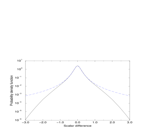
Figure 1: The probability distribution function of scalar differences with and without friction (solid and dashed lines). The specific parameters are $d=1$, $\xi=1$, ${\cal S}^{2}={\cal C}^{2}={{}_{1}\over{}^{2}}$, $\chi(0)=1$, $\alpha=2$, and $r=0.01$.

It is interesting to look at this saturation from the point of view of the p.d.f. ${\cal P}^{\theta}(\vartheta,r)$, defined as in the relation (5.15). The equation for ${\cal P}^{\theta}$ can be derived by the same procedure as in the previous section. Its stationary version reads

$$-M_{2}{\cal P}^{\theta}\,+\,\alpha\hskip 0.71114pt\,\partial_{\vartheta}\left(\vartheta{\cal P}^{\theta}\right)+\,(\chi(0)-\chi)\,\partial_{\vartheta}^{2}\,{\cal P}^{\theta}\ =\ 0\hskip 0.71114pt.$$ (6.15)

For the scales $r\gg L$ of interest to us here, $\chi$ can be neglected with respect to $\chi(0)$. The relevant informations on the p.d.f. ${\cal P}^{\theta}$ are conveniently extracted by expanding the function ${\cal P}^{\theta}$ in a series

$${\cal P}^{\theta}(\vartheta,r)=\sqrt{{{}_{\alpha}\over{}^{2\pi\hskip 0.71114pt\chi(0)}}}\,{\rm e}^{-{\alpha\vartheta^{2}\over 2\chi(0)}}\sum_{k=0}^{\infty}d_{2k}(r)\,H_{2k}\left(\sqrt{{{}_{\alpha}\over{}^{2\chi(0)}}}\,\vartheta\right)$$ (6.16)

of the Hermite polynomials $H_{2k}$. The coefficients $d_{2k}$ can be obtained by plugging the expansion (6.16) into Eq.  (6.15) and using well-known properties of Hermite functions. One obtains

$$d_{0}(r)=1\hskip 0.71114pt,\qquad d_{2k}(r)={{}_{(-1)^{k}}\over{}^{\Gamma(b)}}{{}_{1}\over{}^{k!\,\hskip 0.71114pt2^{b-1+2k}}}\,z_{k}^{b}\hskip 0.71114pt\,K_{b}(z_{k})\hskip 0.71114pt,$$ (6.17)

where $z_{k}$ is defined in Eq.  (6.6). At scales $r\gg\eta_{{}_{f}}$, friction dominates and the p.d.f. tends to a Gaussian form. In the inverse cascade convective range $L\ll r\ll\eta_{{}_{f}}$, the solution (5.17) remains valid as long as $\vartheta^{2}\ll{\chi(0)\over\alpha}$, while the power-law tails are cut by an exponential fall off. The situation is exemplified in Fig. 1. The scaling behavior (6.10) of the structure functions is then easy to grasp: for ${N\over 2}<b$, the dominant contribution comes from the scale invariant part of the p.d.f., resulting in the normal scaling, whereas for ${N\over 2}\geq b$, the leading contribution comes from the region around $\theta^{2}={\chi(0)\over\alpha}$, with the tails cut out by friction. The dominant behavior can be captured by simply calculating the moments with the scale-invariant p.d.f. (5.17) cut at $\vartheta^{2}={\chi(0)\over\alpha}$.

7 Advection of a density

The time $t\,$ 2-point function of the scalar $\rho$, whose advection is governed by Eq.  (1.10), may be studied similarly as for the tracer $\theta$, see [19, 28]. For the free decay of the 2-point function, we obtain

$$F^{\rho}_{2}(t,r)\equiv\langle\,\rho(t,{{\bf r}})\,\rho(t,{\bf 0})\,\rangle\ =\ \int\limits_{0}^{\infty}P^{0,t}_{2}(r^{\prime},r)\,\,F_{2}^{\rho}(0,r^{\prime})\,\hskip 0.71114ptd\mu_{d}({r^{\prime}})\hskip 0.71114pt,$$ (7.1)

where we have used Eqs.  (2.4) and (2.10), compare to Eq.  (3.1). The evolution (1.10) of the scalar $\rho$ preserves the total mass $\int\rho(t,{{\bf r}})\hskip 0.71114ptd{{\bf r}}$. As a consequence, the mean “total mass squared” per unit volume $m^{2}_{\rho}(t)\equiv\int\langle\hskip 0.71114pt\rho(t,{{\bf r}})\hskip 0.71114pt\rho(t,{\bf 0})\hskip 0.71114pt\rangle\hskip 0.71114ptd{{\bf r}}=\int\limits_{0}^{\infty}F^{\rho}_{2}(t,r)\,d\mu_{d}(r)$ does not change in time in both phases.

In the presence of the stationary forcing, the 2-point function of $\rho$ computed with the use of Eqs.(2.6) and (2.10) becomes

$$F^{\rho}_{2}(t,r)\ =\ \int\limits_{0}^{t}ds\int\limits_{0}^{\infty}P^{s,t}_{2}(r^{\prime},r)\,\hskip 0.71114pt\chi({r^{\prime}})\,\hskip 0.71114ptd\mu_{d}({r^{\prime}})\hskip 0.71114pt,$$ (7.2)

if $\rho=0$ at time zero. It evolves according to the equation

$$\partial_{t}F^{\rho}_{2}\,=\,-(M_{2}^{\kappa})^{*}\hskip 0.71114ptF^{\theta}_{2}\,+\,\chi\hskip 0.71114pt,$$ (7.3)

i.e. similarly to $F^{\theta}_{2}$, see Eq.  (3.3), but with $M_{2}^{\kappa}$ exchanged for its adjoint $(M_{2}^{\kappa})^{*}$, a signature of the duality between the two scalars noticed before.

For $\wp<{{}_{d-2+\xi}\over{}^{2\hskip 0.71114pt\xi}}$, the 2-point function $F^{\rho}_{2}(t,r)$ attains a stationary form given by Eq.  (D.2) of Appendix D for $\kappa>0$ and reducing for $\kappa=0$ to the expression

$$F^{\rho}_{2}(r)\ =\ {{}_{1}\over{}^{(a-1)\hskip 0.71114ptZ}}\,r^{-d+1+a-\xi}\smallint\limits_{r}^{\infty}{r^{\prime}}^{d-a}\,\hskip 0.71114pt\chi(r^{\prime})\,\hskip 0.71114ptdr^{\prime}\hskip 0.71114pt+\hskip 0.71114pt{{}_{1}\over{}^{(a-1)\hskip 0.71114ptZ}}\,r^{-d+2-\xi}\smallint\limits_{0}^{r}{r^{\prime}}^{d-1}\,\hskip 0.71114pt\chi(r^{\prime})\,\hskip 0.71114ptdr^{\prime}\hskip 0.71114pt.\ \quad$$ (7.4)

In particular, $F_{2}^{\rho}(r)$ becomes proportional to $r^{-d+1+a-\xi}$ for small $r$ and diverges at $r=0$, except for the incompressible case when the two scalars coincide. The small $r$ behavior agrees with the result of [19] and, in one dimension, with that of [28]. For large distances $r$, the function $\,F_{2}^{\rho}(r)$ is proportional to $r^{-d+2-\xi}$. In the upper interval ${{}_{d-2+\xi}\over{}^{2\hskip 0.71114pt\xi}}<\wp<{{}_{d}\over{}^{\xi^{2}}}$ of the weakly compressible phase, it is

$$F^{\rho}_{2}(t,r)\hskip 0.71114pt-\hskip 0.71114pt{{}_{(4\hskip 0.71114ptZ^{\prime})^{b}}\over{}^{(1-a)\hskip 0.71114ptZ\,\Gamma({1-b})}}\,\,t^{b}\,r^{-d+1+a-\xi}\smallint\limits_{0}^{\infty}{r^{\prime}}^{d-1}\,\chi(r^{\prime})\,\hskip 0.71114ptdr^{\prime}$$

that reaches the stationary limit still given for $\kappa=0$ by the right hand side of Eq.  (7.4). Thus the 2-point function $F_{2}^{\rho}(t,r)$ is pumped now into the zero mode $r^{-d+1+a-\xi}$ of the operator $M_{2}^{*}$.

The higher order correlation functions of $\rho$, $\,F^{\rho}_{N}(t,\underline{{{\bf r}}})\hskip 0.71114pt\equiv\hskip 0.71114pt\langle\hskip 0.71114pt\prod\limits_{n=1}^{N}\rho(t,{{\bf r}}_{n})\hskip 0.71114pt\rangle$,  are expected to converge for long times to a stationary form for sufficiently small $\xi$ and/or compressibility and to be dominated at short distances by a scaling zero mode $\psi_{0}$ of the operator $M_{N}^{*}$,

$$\psi_{0}(\underline{{{\bf r}}})\ =\ 1\,-\,d\,{\wp}\,\xi\sum\limits_{1\leq n<m\leq N}\ln{|{{\bf r}}_{n}-{{\bf r}}_{m}|}\ +\ {\cal O}(\xi^{2})\hskip 0.71114pt.$$ (7.5)

The zero mode $\psi_{0}$ becomes equal to 1 when $\xi\to 0$. The scaling dimension of $\psi_{0}$ may be easily calculated to the first order in $\xi$ by applying the dilation generator to the left hand side of Eq.  (7.5). It is equal to

$$-\hskip 0.71114pt{{}_{N(N-1)\hskip 0.71114ptd}\over{}^{2}}\hskip 0.71114pt\wp\,\xi\ +{\cal O}(\xi^{2})\ \equiv\ {{}_{N}\over{}^{2}}(2-\xi)\,+\,\Delta^{\rho}_{{}_{N}}\hskip 0.71114pt,$$ (7.6)

which again agrees with the result

$$\Delta^{\rho}_{{}_{N}}\,=\,-\hskip 0.71114ptN\,+\,{{}_{N\hskip 0.71114pt(1-(N-1)\,\wp\hskip 0.71114ptd)}\over{}^{2}}\,\xi\ +\ {\cal O}(\xi^{2})$$

of [19] and with the exact result $\,\Delta^{\rho}_{2}=a-1-d\,$ obtained above. Note the singular behavior of $\psi_{0}(\underline{{{\bf r}}})$ at the origin, at least for small $\xi$.

Finally, in the strongly compressible phase $\wp\geq{d\over\xi^{2}}$, where the second of the expressions (2.30) has to be used for $P_{2}^{s,t}$, we obtain

$$F^{\rho}_{2}(t,r) = \smallint\limits_{0}^{t}ds\smallint\limits_{0}^{\infty}{\rm e}^{-s\hskip 0.71114ptM^{+}_{2}}(r^{\prime},r)\,\hskip 0.71114pt\chi(r^{\prime})\,\hskip 0.71114ptd\mu_{d}(r^{\prime})$$ (7.8)

$$+\ \delta({{\bf r}})\,\smallint\limits_{0}^{t}ds\smallint\limits_{0}^{\infty}[\hskip 0.71114pt1\hskip 0.71114pt-\hskip 0.71114pt\gamma(b,\hskip 0.71114pt{{}_{{r^{\prime}}^{2-\xi}}\over{}^{4\hskip 0.71114ptZ^{\prime}\hskip 0.71114pts}})\,\hskip 0.71114pt\Gamma(b)^{-1}]\,\,\chi(r^{\prime})\,\hskip 0.71114ptd\mu_{d}(r^{\prime})\hskip 0.71114pt.$$

For large times, $F_{2}^{\rho}(t,r)$ is pumped into the singular mode proportional to the delta-function with a constant rate:

$$F^{\rho}_{2}(t,r)\ -\ \delta({{\bf r}})\,\hskip 0.71114ptt\,\hskip 0.71114pt\smallint\limits_{0}^{\infty}\chi(r^{\prime})\,\hskip 0.71114ptd\mu_{d}(r^{\prime})\ \ \mathop{\rightarrow}\limits_{t\to\infty}\ \ {{}_{1}\over{}^{(1-a)\hskip 0.71114ptZ}}\,r^{-d+1+a-\xi}\smallint\limits_{0}^{r}{r^{\prime}}^{d-a}\,\chi(r^{\prime})\,\hskip 0.71114ptdr^{\prime}$$ (7.9)

$$+\ {{}_{1}\over{}^{(1-a)\hskip 0.71114ptZ}}\,r^{-d+2-\xi}\smallint\limits_{r}^{\infty}{r^{\prime}}^{d-1}\,\chi(r^{\prime})\,\hskip 0.71114ptdr^{\prime}\ +\ {{}_{S_{d-1}}\over{}^{(2-\xi)(1+a-\xi)\hskip 0.71114ptZ}}\,\delta({{\bf r}})\smallint\limits_{0}^{\infty}{r^{\prime}}^{d+1-\xi}\,\hskip 0.71114pt\chi(r^{\prime})\,\hskip 0.71114ptdr^{\prime}$$ (7.10)

(except for $\wp={d\over\xi^{2}}$), compare to Eqs.  (3.14) and (3.16). Its non-singular part, however, stabilizes and becomes proportional to $r^{-d+2-\xi}$ for small $r$ and to $r^{-d+1+a-\xi}$ for large $r$. Note the inversion of the powers as compared with the weakly compressible phase.

The mean total mass squared of $\rho$ per unit volume, $m^{2}_{\rho}$, exhibits in the presence of forcing a position-space cascade analogous to the wavenumber-space cascade of the energy $e_{{}_{\theta}}$. Let us localize $m^{2}_{\rho}$ in space by defining its amount between the radii $r$ and $R$ as

$$m^{2}_{\rho;\hskip 0.71114ptr,R}(t)\ =\ \smallint\limits_{r}^{R}F^{\rho}_{2}(t,r^{\prime})\,\hskip 0.71114ptd\mu_{d}(r^{\prime})\hskip 0.71114pt.$$ (7.11)

Integrating the evolution equation (7.3) for $F^{\rho}_{2}$ with the radial measure $d\mu_{d}$ from $r$ to $R$, and using the explicit form of $\,M_{2}^{*}=-\hskip 0.71114ptZ\,r^{-d+1}\hskip 0.71114pt\partial_{r}\hskip 0.71114ptr^{a}\hskip 0.71114pt\partial_{r}\hskip 0.71114ptr^{d-1-a+\xi}\hskip 0.71114pt,$  we obtain the relation

$$\partial_{t}\,m^{2}_{\rho;\hskip 0.71114ptr,R}(t)\ =\ Z\hskip 0.71114ptS_{d-1}\hskip 0.71114pt{r^{\prime}}^{a}\hskip 0.71114pt\partial_{r^{\prime}}\hskip 0.71114pt{r^{\prime}}^{d-1-a+\xi}\,F^{\rho}_{2}(t,r^{\prime})\Big{|}_{r}^{R}\ +\ \smallint\limits_{r}^{R}\chi(r^{\prime})\,\hskip 0.71114ptd\mu_{d}(r^{\prime})$$ (7.12)

expressing the local balance of the total mass squared, provided that we interpret $\smallint\limits_{r}^{R}\chi(r^{\prime})\,\hskip 0.71114ptd\mu_{d}(r^{\prime})$ as the injection rate of $m^{2}_{\rho}$ in the radii between $r$ and $R$ and

$$Z\hskip 0.71114ptS_{d-1}\hskip 0.71114ptr^{a}\hskip 0.71114pt\partial_{r}\hskip 0.71114ptr^{d-1-a+\xi}\,F^{\rho}_{2}(r,t)\,\equiv\,\Phi(r)$$

as the flux of $m^{2}_{\rho}$ into the radii $\leq r$. In the weakly compressible phase $\wp<{{}_{d}\over{}^{\xi^{2}}}$ and in the stationary state, $\Phi(r)=-\hskip 0.71114pt\smallint\limits_{0}^{r}\chi(r^{\prime})\,\hskip 0.71114ptd\mu_{d}(r^{\prime})$ so that the flux is constant for $r$ much larger than the injection scale $L$ and it is directed towards bigger radii. On the other hand, in the strongly compressible phase $\wp>{{}_{d}\over{}^{\xi^{2}}}$, one has the equality $\Phi(r)=\smallint\limits_{r}^{\infty}\chi(r^{\prime})\,\hskip 0.71114ptd\mu_{d}(r^{\prime})$ so that the flux is directed towards smaller distances. It eventually feeds into the singular mode all of $m^{2}_{\rho}$ injected by the source. As we see, the two phases differ also by the direction of the cascade of the total mass squared of $\rho$.

8 Conclusions

We have studied the Gaussian ensemble of compressible $d$-dimensional fluid velocities decorrelated in time and with spatial behavior characterized by the fractional Hölder exponent ${\xi\over 2}$. We have shown that the Lagrangian trajectories of fluid particles in such an ensemble exhibit very different behavior, depending on the degree of compressibility $\wp$ of the velocity field. For $\wp<{{}_{d}\over{}^{\xi^{2}}}$, i.e. $b$ defined in (2.20) smaller than unity, the infinitesimally close trajectories separate in finite time, implying that the dissipation remains finite in the limit when the molecular diffusivity $\kappa\to 0$ and that the energy is transferred towards small scales in a direct cascade process. The constancy of the flux at small scales leads to a normal scaling behavior $r^{2-\xi}$ of the second order structure function $S^{\theta}_{2}(r)$ for $r\ll L$ (the typical scale where the energy is injected). For $b$ negative (which includes the incompressible case), as the system evolves, the dissipation rate tends to the injection rate rapidly enough to ensure that the energy $\langle\theta^{2}\rangle$ remains finite. The non-constant zero mode $r^{(2-\xi)b}$ controls the decay of $S^{\theta}_{2}(r)$ to its finite asymptotic value $2\langle\theta^{2}\rangle$ at large $r$. Conversely, for $0\leq b<1$, the dissipation rate tends to the injection rate very slowly, $\propto t^{-(1-b)}$, and the energy is thus increasing with time as $t^{b}$. The structure function $S^{\theta}_{2}(r)$ grows now at large distances as the zero mode $r^{(2-\xi)b}$. For $b\geq 1$, coinciding particles do not separate and, in fact, separated particles collapse in a finite time. The consequences are that the dissipative anomaly is absent and that the energy is entirely transferred toward larger and larger scales in an inverse cascade process. The threshold $b=1$ corresponds to the crossing of the exponents: $(2-\xi)b$ of the non-constant zero mode and $2-\xi$ of the constant-flux-of-energy solution. The picture is the mirror image of the one for the direct cascade, with the first exponent controlling now the small scale behavior and the second one appearing at the large scales. A sketch of the three possible situations is presented in Fig. 2.

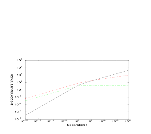
Figure 2: The second-order structure function $S^{\theta}_{2}(r)$ vs $r$ for $\xi=1.8$ and $d=3$ in the three different regimes $b=-2$ (dot-dashed line), $b=0.5$ (dashed line) and $b=2$ (solid line).

Concerning higher order correlations in the strongly compressible phase $b\geq 1$, we have shown that the inverse energy cascade is self-similar, i.e. without intermittency. The effects of a large scale friction reintroduce, however, an anomalous scaling of the structure functions that do not thermalize without friction. They were exhibited in the explicit expressions for the p.d.f.’s of the tracer differences. As for the scalar density, the different behaviors of the Lagrangian trajectories were shown to result in the inverse or in the direct cascade of the total mass squared in, respectively, the weakly and the strongly compressible phase. As explained in Introduction, we expect the explosive separation of the Lagrangian trajectories and/or their collapse to persist in more realistic ensembles of fully turbulent velocities and to play a crucial role in the determination of statistical properties of the flows at high Reynolds numbers.

Acknowledgements.  M. V. was partially supported by C.N.R.S. GdR “Mécanique des Fluides Géophysiques et Astrophysiques”.

Appendix A

Let us consider the operator $M_{2}$ of Eq.  (2.17) on the half-line $[r_{0},\infty[$, $r_{0}>0$, with the Neumann boundary condition $\partial_{r}\hskip 0.71114ptf(r_{0})=0$. By the relation (2.19), this means that we have to consider the operator $N_{2}$ on $[u_{0},\infty[$ with the boundary condition

$$\partial_{u}\hskip 0.71114ptu^{b-{{}_{1}\over{}^{2}}}\hskip 0.71114pt\varphi(u)|_{{}_{u=u_{0}}}=0$$ (A.1)

for $u_{0}=r_{0}^{2-\xi\over 2}$. For non-integer $b$, the corresponding eigen-functions of $N_{2}$ are

$$\varphi_{E,u_{0}}(u)\ =\ C_{1}(u_{0})\,u^{{}_{1}\over{}^{2}}\hskip 0.71114ptJ_{-b}(\widetilde{u})\,+\,C_{2}(u_{0})\,u^{{}_{1}\over{}^{2}}\hskip 0.71114ptJ_{b}(\widetilde{u})$$ (A.2)

with $\widetilde{u}\equiv{\sqrt{E/Z^{\prime}}}\hskip 0.71114ptu\hskip 0.71114pt,$  see Eq.  (2.21). Since

$$J_{{b}}(z)\ =\ {{}_{1}\over{}^{2^{b}\,\Gamma(1+{b})}}\,z^{b}\,(1+{\cal O}(z^{2}))\hskip 0.71114pt,$$ (A.3)

the boundary condition (A.1) implies that

$$C_{1}(u_{0})\,{\cal O}(\widetilde{u}_{0})\,+\,C_{2}(u_{0})\,{\cal O}({\widetilde{u}_{0}}^{2b-1})\ =\ 0\hskip 0.71114pt.$$ (A.4)

As a result, for (non-integer) $b<1$, $\,\lim\limits_{u_{0}\to 0}\,{{}_{C_{2}(u_{0})}\over{}^{C_{1}(u_{0})}}=\,0\,$ so that in the limit we obtain the eigen-functions of the operator $N_{2}^{-}$. For (non-integer) $b>1$, however, $\,\lim\limits_{u_{0}\to 0}\,{{}_{C_{1}(u_{0})}\over{}^{C_{2}(u_{0})}}=\,0\,$ and the eigen-functions tend to those of $N_{2}^{+}$. The extension to the case of integer $b$ is equally easy.

Appendix B

Let us give here the explicit form of the integrals of the kernels ${\rm e}^{-t\hskip 0.71114ptM^{\mp}_{2}}(r,r^{\prime})$ against powers of $r^{\prime}$. A direct calculation shows that for $\mu\geq 0$ and, respectively, $b<1$ and $b>-1$,

$$\int\limits_{0}^{\infty}{\rm e}^{-t\hskip 0.71114ptM_{2}^{-}}(r,r^{\prime})\,\,{r^{\prime}}^{\mu}\,d\mu_{d}({r^{\prime}}) = {{}_{\Gamma(1+{\mu\over 2-\xi}-b)}\over{}^{\Gamma(1-b)}}\,\left(4\hskip 0.71114ptZ^{\prime}\hskip 0.71114ptt\right)^{\mu\over 2-\xi}$$ (B.2)

$$\cdot\,\,{}_{{}_{1}}F_{{}_{1}}(-{{}_{\mu}\over{}^{2-\xi}},\hskip 0.71114pt1-b,\hskip 0.71114pt-{{}_{r^{2-\xi}}\over{}^{4\hskip 0.71114ptZ^{\prime}\hskip 0.71114ptt}})\hskip 0.71114pt,$$

$$\int\limits_{0}^{\infty}{\rm e}^{-t\hskip 0.71114ptM_{2}^{+}}(r,r^{\prime})\,\,{r^{\prime}}^{\mu}\,d\mu_{d}({r^{\prime}}) = {{}_{\Gamma(1+{\mu\over 2-\xi})}\over{}^{\Gamma(1+b)}}\,\left(4\hskip 0.71114ptZ^{\prime}\hskip 0.71114ptt\right)^{{\mu\over 2-\xi}-b}\,\hskip 0.71114ptr^{1-a}$$ (B.4)

$$\cdot\,\,_{{}_{1}}F_{{}_{1}}(-{{}_{\mu}\over{}^{2-\xi}}+b,\hskip 0.71114pt1+b,\hskip 0.71114pt-{{}_{r^{2-\xi}}\over{}^{4\hskip 0.71114ptZ^{\prime}\hskip 0.71114ptt}})\hskip 0.71114pt.$$

A direct calculation gives also the asymptotic expansion of the kernels ${\rm e}^{-t\hskip 0.71114ptM_{2}^{\mp}}(r,r^{\prime})$ at small $r$:

$${\rm e}^{-t\hskip 0.71114ptM_{2}^{\mp}}(r,r^{\prime})\ \ \ =\ \ \ {{}_{2-\xi}\over{}^{S_{d-1}\hskip 0.71114pt\Gamma(1\mp b)}}\,\left\{\matrix{{r^{\prime}}^{-d+2-\xi}\cr r^{1-a}\,{r^{\prime}}^{-d+1+a-\xi}}\right\}$$ (B.5)

$$\hskip 71.13188pt\cdot\ \sum\limits_{j=0}^{\infty}{{}_{(-1)^{j}\,r^{(2-\xi)j}}\over{}^{j!\,(1\mp b)\cdots(j\mp b)\,(4\hskip 0.71114ptZ^{\prime}\hskip 0.71114ptt)^{1+j}}}\ \,{{}_{d}\over{}^{(dz)^{j}}}\,(\hskip 0.71114ptz^{j\mp b}\hskip 0.71114pt{\rm e}^{-z}\hskip 0.71114pt)\bigg{|}_{\hskip 0.71114ptz\,=\hskip 0.71114pt{{r^{\prime}}^{2-\xi}\over 4\hskip 0.71114ptZ^{\prime}\hskip 0.71114ptt}}\hskip 0.71114pt.\hskip 42.67912pt$$ (B.6)

An expansion around $r^{\prime}=0$ may be obtained similarly.

Appendix C

Here we shall consider the long time behavior of the integral of the heat kernel of the operator $M_{2}^{-}$:

$$X(t,r,r^{\prime})\ \equiv\ \smallint\limits_{0}^{t}{\rm e}^{-s\hskip 0.71114ptM_{2}^{-}}(r,r^{\prime})\,ds\hskip 0.71114pt.$$ (C.1)

Using the explicit form (2.25) of the heat kernel ${\rm e}^{-s\hskip 0.71114ptM_{2}^{-}}(r,r^{\prime})$, we may rewrite the last definition as

$$X(t,r,r^{\prime})\ =\ \smallint\limits_{0}^{t}ds\smallint\limits_{0}^{\infty}{\rm e}^{-sE}\,E^{-{b}}\,G(E;r,r^{\prime})\,dE\hskip 0.71114pt,$$ (C.2)

where

$$G(E,r,r^{\prime})\hskip 0.71114pt=\hskip 0.71114pt{{}_{1}\over{}^{(2-\xi)\hskip 0.71114ptZ\hskip 0.71114ptS_{d-1}}}\,r^{1-a\over 2}\,E^{{b}}\,J_{-{b}}({\sqrt{E/Z^{\prime}}}\hskip 0.71114pt{r^{2-\xi\over 2}})\,\hskip 0.71114ptJ_{-{b}}({\sqrt{E/Z^{\prime}}}\hskip 0.71114pt{{r^{\prime}}^{2-\xi\over 2}})\,\hskip 0.71114pt{r^{\prime}}^{-d+{3\over 2}+{a\over 2}-\xi}\hskip 0.71114pt.\ \quad$$ (C.3)

Note that, by virtue of the relation (A.3), $\,G(0,r,r^{\prime})={{}_{(2-\xi)\hskip 0.71114pt(4\hskip 0.71114ptZ^{\prime})^{{b}-1}}\over{}^{\Gamma(1-{b})^{2}\hskip 0.71114ptS_{d-1}}}\,{r^{\prime}}^{-d+1+a-\xi}\equiv G_{0}(r^{\prime})\,$ and is independent of $r$. For finite times, the integration by parts, accompanier by the changes of variable $sE\leftrightarrow E$ gives the following identity:

$${b}\hskip 0.71114ptX(t,r,r^{\prime})\hskip 0.71114pt=\hskip 0.71114ptt^{b}\smallint\limits_{0}^{\infty}{\rm e}^{-E}\hskip 0.71114ptE^{-{b}}\hskip 0.71114ptG(t^{-1}E,r,r^{\prime})\hskip 0.71114ptdE\hskip 0.71114pt+\hskip 0.71114pt\smallint\limits_{0}^{t}ds\smallint\limits_{0}^{\infty}{\rm e}^{-sE}\hskip 0.71114ptE^{1-{b}}\hskip 0.71114pt\partial_{{}_{E}}G(E,r,r^{\prime})\hskip 0.71114ptdE\hskip 0.71114pt.\quad$$ (C.4)

For $b<0$, the $t\to\infty$ limit of $X(t,r,r^{\prime})$ exists and defines the kernel $(M_{2}^{-})^{-1}(r,r^{\prime})$:

$$\lim\limits_{t\to\infty}\,\,{b}\,X(t,r,r^{\prime}) = {b}\smallint\limits_{0}^{\infty}E^{-{b}-1}\,G(E,r,r^{\prime})\,dE$$ (C.5)

$$= -\hskip 0.71114pt{{}_{1}\over{}^{(2-\xi)\hskip 0.71114ptZ\,S_{d-1}}}\cases{\hbox to113.81102pt{${r^{\prime}}^{-d+2-\xi}$\hfill}{\rm for\ }r\leq r^{\prime}\hskip 0.71114pt,\cr\hbox to113.81102pt{$r^{(2-\xi)b}\hskip 0.71114pt{r^{\prime}}^{-d+(2-\xi)(1-b)}$\hfill}{\rm for\ }r\geq r^{\prime}\hskip 0.71114pt,}$$ (C.6)

compare to Eq.  (3.5). The last expression has been obtained by the direct integration and the condition $b<0$ was required by the convergence at zero of the $E$-integral (the kernels $(M_{2}^{\pm})^{-1}(r,r^{\prime})$ may be also found easily by gluing the zero modes of $M_{2}^{\pm}$). Note that the right hand side is a real analytic function of ${b}={{1-a}\over{2-\xi}}$. Now Eq.  (C.4) implies that

$$\lim\limits_{t\to\infty}\,\left[\hskip 0.71114pt{b}\,X(t,r,r^{\prime})\,-\,\Gamma(1-{b})\,G_{0}(r^{\prime})\,t^{b}\hskip 0.71114pt\right]\ =\ \smallint\limits_{0}^{\infty}E^{-{b}}\,\partial_{{}_{E}}G(E,r,r^{\prime})\,dE$$ (C.7)

exists for ${b}<1$ and is also real analytic in ${b}$. On the other hand, it coincides with the long time limit in Eq.  (C.6) for ${b}<0$ and, consequently, must be given by the right hand side of this equation for all ${b}<1$. The same arguments work after the integration of the above expressions against $\chi(r^{\prime})\hskip 0.71114ptd\mu_{d}(r^{\prime})$ and hence the convergence of the expression (3.10) when $t\to\infty$.

Appendix D

It is easy to give the exact expressions for the stationary 2-point functions of the scalars $\theta$ and $\rho$ for $\wp<{{}_{d-2+\xi}\over{}^{2\hskip 0.71114pt\xi}}$ in the presence of positive diffusivity $\kappa$. They are

$$F^{\theta}_{2}(r) = {{}_{1}\over{}^{Z\,S_{d-1}}}\smallint\limits_{r}^{\infty}f(r^{\prime})\,g(r^{\prime})\,\hskip 0.71114pt\chi(r^{\prime})\,\hskip 0.71114ptd\mu_{d}(r^{\prime})\,+\,{{}_{1}\over{}^{Z\,S_{d-1}}}\,\hskip 0.71114ptg(r)\smallint\limits_{0}^{r}f(r^{\prime})\,\hskip 0.71114pt\chi(r^{\prime})\,\hskip 0.71114ptd\mu_{d}(r^{\prime})\hskip 0.71114pt,$$ (D.1)

$$F^{\rho}_{2}(r) = {{}_{1}\over{}^{Z\,S_{d-1}}}\,\hskip 0.71114ptf(r)\smallint\limits_{r}^{\infty}g(r^{\prime})\,\hskip 0.71114pt\chi(r^{\prime})\,\hskip 0.71114ptd\mu_{d}(r^{\prime})\,+\,{{}_{1}\over{}^{Z\,S_{d-1}}}\,\hskip 0.71114ptf(r)\,g(r)\smallint\limits_{0}^{r}\chi(r^{\prime})\,\hskip 0.71114ptd\mu_{d}(r^{\prime})\hskip 0.71114pt,$$ (D.2)

where

$$f(r)\hskip 0.71114pt=\hskip 0.71114pt(r^{\xi}+{{}_{2\hskip 0.71114pt\kappa}\over{}^{Z}})^{{}^{-d+1+a-\xi\over\xi}}\qquad{\rm and}\qquad g(r)\hskip 0.71114pt=\hskip 0.71114pt\smallint\limits_{r}^{\infty}f(\zeta)^{-1}\,{{}_{\zeta^{-d+1}}\over{}^{\zeta^{\xi}+{2\hskip 0.71114pt\kappa\over Z}}}\,d\zeta\hskip 0.71114pt.$$ (D.3)

In the limit $\kappa\to 0$ these expressions pass into Eq.  (3.5) and (7.4), respectively. For ${{}_{d-2+\xi}\over{}^{2\hskip 0.71114pt\xi}}<\wp<{{}_{d}\over{}^{\xi^{2}}}$, similarly as at $\kappa=0$, the 2-point functions $F_{2}^{\theta}(t,r)$ and $F_{2}^{\rho}(t,r)$ are pumped into the constant and the $f(r)$ zero modes of $M_{2}^{\kappa}$ and $(M_{2}^{\kappa})^{*}$, respectively, and do not reach stationary limits, although the 2-point structure function of the tracer does. For $\wp\geq{d\over\xi^{2}}$ the pumping into the zero modes reaches a constant rate. In the limit $\kappa\to 0$, the zero mode $f(r)$ into which $F_{2}^{\rho}$ is pumped goes to $r^{-d+1+a-\xi}$ for $\wp<{d\over\xi^{2}}$ but becomes the delta-function $\delta({{\bf r}})$ for $\wp>{d\over\xi^{2}}$.

Appendix E

Let us prove the explicit expression (5.3) for the even structure functions in the strongly compressible regime. Note that

$$S^{\theta}_{{}_{N}}(t,r)\ =\ \sum\limits_{Q\subset\{1,\dots,N\}}(-1)^{|Q^{c}|}\,\,F^{\theta}_{{}_{N}}(t,({{\bf r}})_{{}_{q\in Q}},({\bf 0})_{{}_{q\in Q^{c}}})$$ (E.1)

where $Q^{c}$ stands for the complement of $Q$. In the strongly compressible phase, by the multiple application of Eq.  (5.1), we infer that

$$P^{t,s}_{{}_{N}}(({{\bf r}})_{{}_{q\in Q}},({\bf 0})_{{}_{q\in Q^{c}}};\hskip 0.71114pt\underline{{{\bf r}}^{\prime}}) = \int P^{t,s}_{2}({{\bf r}},{\bf 0};\hskip 0.71114pt{{\bf r}}^{\prime\prime}_{1},{{\bf r}}^{\prime\prime}_{2})$$ (E.3)

$$\cdot\ \prod\limits_{q\in Q}\delta({{\bf r}}^{\prime\prime}_{1}-{{\bf r}}^{\prime}_{q})\,\prod\limits_{q\in Q^{c}}\delta({{\bf r}}^{\prime\prime}_{2}-{{\bf r}}^{\prime}_{q})\,\,d{{\bf r}}^{\prime\prime}_{1}\,\hskip 0.71114ptd{{\bf r}}^{\prime\prime}_{2}\hskip 0.71114pt.$$

Substituting Eq.  (4.7) into the expression (E.1) and using the relations (E.3), we obtain

$$S^{\theta}_{{}_{N}}(t,r) = \sum\limits_{1\leq n<m\leq N}\int\limits_{0}^{t}ds\int P_{2}^{t,s}({{\bf r}},{\bf 0};\hskip 0.71114pt{{\bf r}}^{\prime\prime}_{1},{{\bf r}}^{\prime\prime}_{2})$$ (E.8)

$$\cdot\,\bigg{(}\sum\limits_{\{n,m\}\subset Q\subset\{1,\dots,N\}}(-1)^{|Q^{c}|}\ F^{\theta}_{{}_{N-2}}(s,({{\bf r}}^{\prime\prime}_{1})_{{}_{q\in Q\setminus\{n,m\}}},({{\bf r}}^{\prime\prime}_{2})_{{}_{q\in Q^{c}}})\ \chi(0)$$

$$\ \ +\sum\limits_{n\in Q\subset\{1,\dots,N\}\setminus\{m\}}(-1)^{|Q^{c}|}\ F^{\theta}_{{}_{N-2}}(s,({{\bf r}}^{\prime\prime}_{1})_{{}_{q\in Q\setminus\{n\}}},({{\bf r}}^{\prime\prime}_{2})_{{}_{q\in Q^{c}\setminus\{m\}}})\ \chi({|{{\bf r}}^{\prime\prime}_{1}-{{\bf r}}^{\prime\prime}_{2}|})$$

$$\ \ +\sum\limits_{m\in Q\subset\{1,\dots,N\}\setminus\{n\}}(-1)^{|Q^{c}|}\ F^{\theta}_{{}_{N-2}}(s,({{\bf r}}^{\prime\prime}_{1})_{{}_{q\in Q\setminus\{m\}}},({{\bf r}}^{\prime\prime}_{2})_{{}_{q\in Q^{c}\setminus\{n\}}})\ \chi({|{{\bf r}}^{\prime\prime}_{1}-{{\bf r}}^{\prime\prime}_{2}|})$$

$$\ \ +\sum\limits_{Q\subset\{1,\dots,N\}\setminus\{n,m\}}(-1)^{|Q^{c}|}\ F^{\theta}_{{}_{N-2}}(s,({{\bf r}}^{\prime\prime}_{1})_{{}_{q\in Q}},({{\bf r}}^{\prime\prime}_{2})_{{}_{q\in Q^{c}\setminus\{n,m\}}})\ \chi(0)\bigg{)}\,d{{\bf r}}^{\prime\prime}_{1}\,d{{\bf r}}^{\prime\prime}_{2}$$

$$= \ N(N-1)\,\smallint\limits_{0}^{t}ds\smallint\limits_{0}^{\infty}P_{2}^{t,s}(r,r^{\prime})\,\,S^{\theta}_{{}_{N-2}}(s,r^{\prime})\,\,(\chi(0)-\chi({r^{\prime}}))\,\,d\mu_{d}({r^{\prime}})\hskip 0.71114pt,$$ (E.11)

which is the sought relation.

References

- [1] A. N. Kolmogorov, The local structure of turbulence in incompressible viscous fluid for very large reynolds’ numbers. C. R. Acad. Sci. URSS 30, 301-305 (1941).
- [2] R. H. Kraichnan, Inertial ranges in two-dimensional turbulence, Phys. Fluids 10, 1417-1423 (1967).
- [3] J. Paret & P. Tabeling, Intermittency in the 2D inverse cascade of energy: experimental observations, Phys. Fluids 10, 3126-3136 (1998).
- [4] L. M. Smith & V. Yakhot, Bose condensation and small-scale structure generation in a random force driven 2D turbulence, Phys. Rev. Lett. 71, 352-355 (1993).
- [5] A. Babiano, On non-homogeneous two-dimensional inverse cascade of energy, preprint, (1998).
- [6] D. Ruelle & F. Takens, On the nature of turbulence, Comm. Math. Phys. 20, 167-192 (1971).
- [7] T. Bohr, M. H. Jensen, G. Paladin & A. Vulpiani, “Dynamical Systems Approach to Turbulence”, Cambridge University Press, Cambridge 1988.
- [8] D. Bernard, K. Gawȩdzki & A. Kupiainen, Slow modes in passive advection, J. Stat. Phys. 90, 519-569 (1998).
- [9] U. Frisch, A. Mazzino & M. Vergassola, Intermittency in passive scalar advection, Phys. Rev. Lett. 80, 5532-5535 (1998).
- [10] K. Gawȩdzki, Intermittency of Passive Advection, in “Advances in Turbulence VII”, U. Frisch ed. Kluwer Acad. Publ. 1998, pp. 493-502.
- [11] R. H. Kraichnan, Anomalous scaling of a randomly advected passive scalar, Phys. Rev. Lett. 52, 1016-1019 (1994).
- [12] M. Vergassola & M. Avellaneda, Scalar transport in compressible flow, Physica D 106, 148-166 (1997).
- [13] Ya. G. Sinai, Limit behavior of one dimensional random walk in random environment, Theor. Prob. Appl. 27, 247-258 (1982).
- [14] D. Bernard & K. Gawȩdzki, Scaling and Exotic Regimes in Decaying Burgers Turbulence, chao-dyn/9805002.
- [15] M. Chertkov, I. Kolokolov & M. Vergassola, Inverse versus direct cascades in turbulent advection, Phys. Rev. Lett. 80, 512-515 (1998).
- [16] M. Chertkov, I. Kolokolov & M. Vergassola, Inverse cascade and intermittency of passive scalar in 1d smooth flow, Phys. Rev. E 56, 5483-5499 (1997).
- [17] D. Biskamp & U. Bremer, Dynamics and statistics of inverse cascade processes in 2D magnetohydrodynamic turbulence, Phys. Rev. Lett. 72, 3819-3822 (1993).
- [18] R. H. Kraichnan, Small-scale structure of a scalar field convected by turbulence, Phys. Fluids 11, 945-963 (1968).
- [19] L. Ts. Adzhemyan & N. V. Antonov, Renormalization group and anomalous scaling in a simple model of passive scalar advection in compressible flow, chao-dyn/9806004.
- [20] M. Reed & B. Simon, “Methods of Modern Mathematical Analysis, II. Fourier Analysis, Self-Adjointness”, Academic Press, London 1980.
- [21] Y. Le Jan & O. Raimond, Solutions statistiques fortes des équations différentielles stochastiques, preprint (1998).
- [22] A. Gamba & I. Kolokolov, The Lyapunov spectrum of continuous product of random matrices. J. Stat. Phys. 85, 489-499 (1996).
- [23] K. Gawȩdzki & A. Kupiainen, Universality in turbulence : an exactly soluble model, in “Low-Dimensional Models in Statistical Physics and Quantum Field Theory”, H. Grosse and L. Pittner eds., Springer, Berlin 1996, pp. 71-105.
- [24] B. Shraiman & E. Siggia, Lagrangian path integrals and fluctuations in random flow, Phys. Rev. E 49, 2912-2927 (1994).
- [25] U. Frisch, “Turbulence: The Legacy of A. N. Kolmogorov”, Cambridge Univ. Press, Cambridge 1995.
- [26] D. Bernard, K. Gawȩdzki & A. Kupiainen, Anomalous scaling in the -point functions of the passive scalar, Phys. Rev. E 54, 2564-2572 (1996).
- [27] M. Chertkov, On how the joint interaction of two innocent partners (smooth advection and linear damping) produces a strong intermittency, Phys. Fluids 10, 3017-3019 (1998).
- [28] M. Vergassola & A. Mazzino, Structures and intermittency in a passive scalar model, Phys. Rev. Lett. 79, 1849-1852 (1997).