Quantum Phase Transitions
in
2d Quantum Liquids

Notation

We adopt Feynman’s notation and denote a spacetime point by $x=x_{\mu}=(t,{\bf x})$, $\mu=0,1,\cdots,d$, with $d$ the number of space dimensions, while the energy $k_{0}$ and momentum ${\bf k}$ of a particle will be denoted by $k=k_{\mu}=(k_{0},{\bf k})$. The time derivative $\partial_{0}=\partial/\partial t$ and the gradient $\nabla$ are sometimes combined in a single vector $\tilde{\partial}_{\mu}=(\partial_{0},-\nabla)$. The tilde on $\partial_{\mu}$ is to alert the reader for the minus sign appearing in the spatial components of this vector. We define the scalar product $k\cdot x=k_{\mu}x_{\mu}=k_{0}t-{\bf k}\cdot{\bf x}$ and use Einstein’s summation convention. Because of the minus sign in the definition of the vector $\tilde{\partial}_{\mu}$ it follows that $\tilde{\partial}_{\mu}a_{\mu}=\partial_{0}a_{0}+\nabla\cdot{\bf a}$, with $a_{\mu}$ an arbitrary vector.

Integrals over spacetime are denoted by

$$\int_{x}=\int_{t,{\bf x}}=\int\mbox{d}t\,\mbox{d}^{d}x,$$

while those over energy and momentum by

$$\int_{k}=\int_{k_{0},{\bf k}}=\int\frac{\mbox{d}k_{0}}{2\pi}\frac{\mbox{d}^{d}k}{(2\pi)^{d}}.$$

When no integration limits are indicated, the integrals are assumed to run over all possible values of the integration variables.

Natural units $\hbar=c=k_{\rm B}=1$ are adopted throughout.

Chapter 1 Prelude

Continuous quantum phase transitions have attracted considerable attention in this decade both from experimentalists as well as from theorists. (For reviews see Refs. [1, 2, 3, 4].) These transitions, taking place at the absolute zero of temperature, are dominated by quantum and not by thermal fluctuations as is the case in classical finite-temperature phase transitions. Whereas time plays no role in a classical phase transition, being an equilibrium phenomenon, it becomes important in quantum phase transitions. The dynamics is characterized by an additional critical exponent, the so-called dynamic exponent, which measures the asymmetry between the time and space dimensions. The natural language to describe these transitions is quantum field theory. In particular, the functional-integral approach, which can also be employed to describe classical phase transitions, turns out to be highly convenient.

The subject is at the border of condensed matter and statistical physics. Typical systems being studied are superfluid and superconducting films, quantum-Hall and related two-dimensional electron systems, as well as quantum spin systems. Despite the diversity in physical content, the quantum critical behavior of these systems shows surprising similarities. It is fair to say that the present theoretical understanding of most of the experimental results is scant.

The purpose of these Lectures is to provide the reader with a framework for studying quantum phase transitions. A central role is played by a repulsively interacting Bose gas at the absolute zero of temperature. The universality class defined by this paradigm is believed to be of relevance to most of the systems studied. Without impurities and a Coulomb interaction, the quantum critical behavior of this system turns out to be surprisingly simple. However, these two ingredients are essential and have to be included. Very general hyperscaling arguments are powerful enough to determine the exact value of the dynamic exponent in the presence of impurities and a Coulomb interaction, but the other critical exponents become highly intractable.

The emphasis in these Lectures will be on effective theories, giving a description of the system under study valid at low energy and small momentum. The rationale for this is the observation that the (quantum) critical behavior of continuous phase transitions is determined by such general features as the dimensionality of space, the symmetries involved, and the dimensionality of the order parameter. It does not depend on the details of the underlying microscopic theory. In the process of deriving an effective theory starting from some microscopic model, irrelevant degrees of freedom are integrated out and only those relevant for the description of the phase transition are retained. Similarities in critical behavior in different systems can, accordingly, be more easily understood from the perspective of effective field theories.

The ones discussed in these Lectures are so-called phase-only theories. The are the dynamical analogs of the familiar O(2) nonlinear sigma model of classical statistical physics. As in that model, the focus will be on phase fluctuations of the order parameter. The inclusion of fluctuations in the modulus of the order parameter is generally believed not to change the critical behavior. Indeed, there are convincing arguments that both the Landau-Ginzburg model with varying modulus and the nonlinear O($n$) sigma model with fixed modulus belong to the same universality class. For technical reasons a direct comparison is not possible, the Landau-Ginzburg model usually being investigated in an expansion around four dimensions, and the nonlinear sigma model in one around two.

In the case of a repulsively interacting Bose gas at the absolute zero of temperature, the situation is particular simple as phase fluctuations are the only type of field fluctuations present.

These Lectures cover exclusively lower-dimensional systems. The reason is that it will turn out that in three space dimensions and higher the quantum critical behavior is in general Gaussian and therefore not very interesting.

Since time and how it compares to the space dimensions is an important aspect of quantum phase transitions, Galilei invariance will play an important role in the discussion.

Chapter 2 Functional Integrals

In these Lectures we shall adopt, unless stated otherwise, the functional-integral approach to quantum field theory. To illustrate the use and power of functional integrals, let us consider one of the simplest models of classical statistical mechanics: the Ising model. It is remarkable that functional integrals can not only be used to describe quantum systems, governed by quantum fluctuations, but also classical systems, governed by thermal fluctuations.

2.1 Ising Model

The Ising model provides an idealized description of an uniaxial ferromagnet. To be specific, let us assume that the spins of some lattice system can point only along one specific crystallographic axis. The magnetic properties of this system can then be modeled by a lattice with a spin variable $s({\bf x})$ attached to every site ${\bf x}$ taking the values $s({\bf x})=\pm 1$. For definiteness we will assume a $d$-dimensional cubic lattice. The Hamiltonian is given by

$$H=-\frac{1}{2}\sum_{{\bf x},{\bf y}}J({\bf x},{\bf y})\,s({\bf x})\,s({\bf y}).$$ (2.1)

Here, ${\bf x}=a\,x_{i}\,{\bf e}_{i}$, with $a$ the lattice constant, $x_{i}$ integers labeling the sites, and ${\bf e}_{i}$ ($i=1,\cdots,d$) unit vectors spanning the lattice. The sums over ${\bf x}$ and ${\bf y}$ extend over the entire lattice, and $J({\bf x},{\bf y})$ is a symmetric matrix representing the interactions between the spins. If the matrix element $J({\bf x},{\bf y})$ is positive, the energy is minimized when the two spins at site ${\bf x}$ and ${\bf y}$ are parallel—they are said to have a ferromagnetic coupling. If, on the other hand, the matrix element is negative, anti-parallel spins are favored—the spins are said to have an anti-ferromagnetic coupling.

The classical partition function $Z$ of the Ising model reads

$$Z=\sum_{\{s({\bf x})\}}{\rm e}^{-\beta H},$$ (2.2)

with $\beta=1/T$ the inverse temperature. The sum is over all spin configurations $\{s({\bf x})\}$, of which there are $2^{N}$, with $N$ denoting the number of lattice sites. To evaluate the partition function we linearize the exponent by introducing an auxiliary $\phi({\bf x})$ at each site via a so-called Hubbard-Stratonovich transformation. Such a transformation generalizes the Gaussian integral

$$\exp\left(-{\textstyle\frac{1}{2}}\beta Js^{2}\right)=\sqrt{\frac{\beta}{2\pi J}}\int_{\phi}\exp\left(-{\textstyle\frac{1}{2}}\beta J^{-1}\phi^{2}+\beta\phi s\right),$$ (2.3)

where the integration variable $\phi$ runs from $-\infty$ to $\infty$. The generalization reads

$$\exp\left[{\textstyle\frac{1}{2}}\beta\sum_{{\bf x},{\bf y}}J({\bf x},{\bf y})\,s({\bf x})\,s({\bf y})\right]=$$

$$\prod_{\bf x}\int\mbox{d}\phi({\bf x})\exp\left[-{\textstyle\frac{1}{2}}\beta\sum_{{\bf x},{\bf y}}J^{-1}({\bf x},{\bf y})\,\phi({\bf x})\,\phi({\bf y})+\beta\sum_{{\bf x}}\phi({\bf x})s({\bf x})\right].$$

Here, $J^{-1}({\bf x},{\bf y})$ is the inverse of the matrix $J({\bf x},{\bf y})$ and we ignored—as will be done throughout these notes—an irrelevant normalization factor in front of the product at the right-hand side. The equation should not be taken too literally. It is an identity only if $J({\bf x},{\bf y})$ is a symmetric positive definite matrix. This is not true for the Ising model since the diagonal matrix elements $J({\bf x},{\bf x})$ are all zero, implying that the sum of the eigenvalues is zero. We will nevertheless use this representation and regard it as a formal one. The partition function now reads

$$Z=\sum_{\{s({\bf x})\}}\prod_{\bf x}\int\mbox{d}\phi({\bf x})\exp\left[-{\textstyle\frac{1}{2}}\beta\sum_{{\bf x},{\bf y}}J^{-1}({\bf x},{\bf y})\,\phi({\bf x})\,\phi({\bf y})+\beta\sum_{\bf x}\phi({\bf x})\,s({\bf x})\right].$$ (2.5)

The spins are decoupled in this representation, so that the sum over the spin configurations is easily carried out with the result

$$Z=\prod_{\bf x}\int\mbox{d}\phi({\bf x})\exp\left(-{\textstyle\frac{1}{2}}\beta\sum_{{\bf x},{\bf y}}J^{-1}({\bf x},{\bf y})\,\phi({\bf x})\,\phi({\bf y})+\sum_{\bf x}\ln\{\cosh\,[\beta\phi({\bf x})]\}\right),$$ (2.6)

ignoring again an irrelevant constant.

The auxiliary field $\phi({\bf x})$ is not devoid of physical relevance. To see this let us first consider its field equation:

$$\phi({\bf x})=\sum_{\bf y}J({\bf x},{\bf y})\,s({\bf y}),$$ (2.7)

which follows from (2.5). This shows that the auxiliary field $\phi({\bf x})$ represents the effect of the other spins at site ${\bf x}$. To make this more intuitive let us study the expectation value of the field. For simplicity, we take only nearest-neighbor interactions into account by setting

$$J({\bf x},{\bf y})=\left\{\begin{array}[]{ll}J&\mbox{if site ${\bf x}$ and ${\bf y}$ are nearest neighbors}\\ 0&\mbox{otherwise,}\end{array}\right.$$ (2.9)

with $J$ positive, so that we have a ferromagnetic coupling between the spins. The model is now translational invariant and the expectation value $\langle s({\bf x})\rangle$ is independent of ${\bf x}$:

$$\langle s({\bf x})\rangle=M.$$ (2.10)

We will refer to $M$ as the magnetization. Upon taking the expectation value of the field equation (2.7),

$$\langle\phi({\bf x})\rangle=2dJM,$$ (2.11)

where $2d$ is the number of nearest neighbors, we see that the expectation value of the auxiliary field represents the magnetization.

A useful approximation often studied is the so-called mean-field approximation. It corresponds to approximating the integral over $\phi({\bf x})$ in (2.6) by the saddle point—the value of the integrand for which the exponent is stationary. This is the case for $\phi({\bf x})$ satisfying the field equation

$$-\sum_{\bf y}J^{-1}({\bf x},{\bf y})\,\phi({\bf y})+\tanh\,[\beta\phi({\bf x})]=0.$$ (2.12)

We will denote the solution by $\phi_{\rm mf}$. In this approximation, the auxiliary field is no longer a fluctuating field taking all possible real values, but a classical one having the value determined by the field equation (2.12). Being a nonfluctuating field, the expectation value $\langle\phi_{\rm mf}({\bf x})\rangle=\phi_{\rm mf}({\bf x})$, and (2.12) yields a self-consistent equation for the magnetization

$$M=\tanh(2d\beta JM),$$ (2.13)

where we assumed a uniform field solution and invoked Eq. (2.11). It is easily seen graphically that the equation has a nontrivial solution when $2d\beta J>1$. If, on the other hand, $2d\beta J<1$ it has only a trivial solution. It follows that

$$\beta^{-1}_{0}=2dJ$$ (2.14)

is the critical temperature separating the ordered low-temperature state with a nonzero magnetization from the high-temperature disordered state where the magnetization is zero.

Let us continue by expanding the Hamiltonian in powers of $\phi$. To this end we note that the term $\ln[\cosh(\beta\phi)]$ in (2.6) has the Taylor expansion

$$\ln[\cosh(\beta\phi)]={\textstyle\frac{1}{2}}\beta^{2}\phi^{2}-{\textstyle\frac{1}{12}}\beta^{4}\phi^{4}+\cdots.$$ (2.15)

Before considering the other term in (2.6), $\sum_{{\bf x},{\bf y}}J^{-1}({\bf x},{\bf y})\,\phi({\bf x})\,\phi({\bf y})$, let us first study the related object $\sum_{{\bf x},{\bf y}}J({\bf x},{\bf y})\,s({\bf x})\,s({\bf y})$ which shows up in the original Ising Hamiltonian (2.1). With our choice (2.9) of the interaction, the Taylor expansion of this object becomes

$$\sum_{{\bf x},{\bf y}}J({\bf x},{\bf y})\,s({\bf x})\,s({\bf y})=J\sum_{\bf x}s({\bf x})\,(2d+a^{2}\nabla^{2}+\cdots)\,s({\bf x}),$$ (2.16)

neglecting higher orders in derivatives. From this it follows that

$$\sum_{{\bf x},{\bf y}}J^{-1}({\bf x},{\bf y})\,\phi({\bf x})\,\phi({\bf y})=J^{-1}\sum_{\bf x}\phi({\bf x})\left(\frac{1}{2d}-\frac{1}{4d^{2}}a^{2}\nabla^{2}+\cdots\right)\phi({\bf x}),$$ (2.17)

and the partition function (2.6) becomes in the small-$\phi$ approximation

$$Z=\prod_{\bf x}\int\mbox{d}\phi({\bf x})\,{\rm e}^{-\beta H},$$ (2.18)

with $H$ the so-called Landau-Ginzburg Hamiltonian

$$H=\sum_{\bf x}\left[\frac{a^{2}}{8d^{2}J}(\nabla\phi)^{2}+\frac{1}{2}\left(\frac{1}{2dJ}-\beta\right)\phi^{2}+\frac{\beta^{3}}{12}\phi^{4}\right].$$ (2.19)

The model has a classical phase transition when the coefficient of the $\phi^{2}$-term changes sign. This happens when $\beta=1/2dJ$ in accord with the conclusion obtained by inspecting the self-consistent equation for the magnetization (2.13).

In the mean-field approximation, the thermal fluctuations around the mean-field configuration are ignored, so that $\phi$ becomes a nonfluctuating field. The functional integral $\prod_{\bf x}\int\mbox{d}\phi({\bf x})$ is approximated by the saddle point.

For future reference we go over to the continuum by letting $a\rightarrow 0$. To this end we replace the discrete sum $\sum_{i}$ by the integral $a^{-d}\int_{\bf x}$, and rescale the field $\phi({\rm x})$,

$$\phi({\bf x})\rightarrow\phi^{\prime}({\bf x})=\sqrt{\frac{\beta a^{2-d}}{4d^{2}J}}\phi({\bf x}),$$ (2.20)

such that the coefficient of the gradient term in the Hamiltonian takes the canonical form of ${\textstyle\frac{1}{2}}$. In this way the Hamiltonian becomes

$$\beta H=\int_{\bf x}\left[\frac{1}{2}(\nabla\phi)^{2}+\frac{1}{2}r_{0}\phi^{2}+\frac{1}{4!}\lambda_{0}\phi^{4}\right],$$ (2.21)

where we dropped the prime on the field; the parameter $r_{0}$ and the coupling constant $\lambda_{0}$ are given by

$$r_{0}=\frac{\beta_{0}^{-2}}{Ja^{2}}(\beta_{0}-\beta),\;\;\;\lambda_{0}=\frac{4\beta^{2}}{J^{2}\beta_{0}^{4}}a^{d-4}.$$ (2.22)

The partition function now reads

$$Z=\int\mbox{D}\phi\,{\rm e}^{-\beta H},$$ (2.23)

where the functional integral $\int\mbox{D}\phi$ denotes the continuum limit of the product of integrals $\prod_{\bf x}\int\mbox{d}\phi({\bf x})$. The last two terms in the integrand of (2.21) constitute the potential ${\cal V}(\phi)$,

$${\cal V}(\phi)=\frac{1}{2}r_{0}\phi^{2}+\frac{1}{4!}\lambda_{0}\phi^{4}.$$ (2.24)

In Fig. 2.1, the potential ${\cal V}(\phi)$ is depicted in the high-temperature phase where $r_{0}>0$, and also in the low-temperature phase where $r_{0}<0$. The minimum of the potential in the low-temperature phase is obtained for a value $\phi\neq 0$, whereas in the high-temperature phase the minimum is always at $\phi=0$.

Figure 2.1: The potential ${\cal V}(\phi)$ of the Ising model in the high-temperature ($r_{0}>0$) and low-temperature ($r_{0}<0$) phase.

2.2 Derivative Expansion

We are interested in taking into account field fluctuations around the mean field $\phi_{\rm mf}$, which is the solution of the field equation obtained from (2.21). To this end we set $\phi=\phi_{\rm mf}+\tilde{\phi}$, and expand the Hamiltonian around the mean field up to second order in $\tilde{\phi}$:

$$\beta H=\beta H_{\rm mf}+\frac{1}{2}\int_{\bf x}\left[(\nabla\tilde{\phi})^{2}+(r_{0}+{\textstyle\frac{1}{2}}\lambda_{0}\phi_{\rm mf}^{2})\tilde{\phi}^{2}\right],$$ (2.25)

where $H_{\rm mf}$ denotes the value of the Hamiltonian (2.21) for $\phi=\phi_{\rm mf}$. Because of the change of variables, the functional integral $\int\mbox{D}\phi$ changes to $\int\mbox{D}\tilde{\phi}$. Since we neglected higher-order terms, the functional integral is Gaussian and easily carried out. The partition function (2.23) becomes in this approximation

$$Z = {\rm e}^{-\beta H_{\rm mf}}\int\mbox{D}\tilde{\phi}\,\exp\left\{-\frac{1}{2}\int_{\bf x}\left[(\nabla\tilde{\phi})^{2}+(r_{0}+{\textstyle\frac{1}{2}}\lambda_{0}\phi_{\rm mf}^{2})\tilde{\phi}^{2}\right]\right\}$$ (2.26)

$$= {\rm e}^{-\beta H_{\rm mf}}\,{\rm Det}^{-1/2}({\bf p}^{2}+r_{0}+{\textstyle\frac{1}{2}}\lambda_{0}\phi_{\rm mf}^{2}),$$

with the derivative ${\bf p}=-i\nabla$. The determinant represents the first corrections to the mean-field expression $\exp(-\beta H_{\rm mf})$ of the partition function due to fluctuations. Using the identity $\mbox{Det(A)}=\exp\left[\mbox{Tr}\,\ln(A)\right]$, we can collect them in the effective Hamiltonian

$$\beta H_{\rm eff}={\textstyle\frac{1}{2}}{\rm Tr}\ln[{\bf p}^{2}+r_{0}+{\textstyle\frac{1}{2}}\lambda_{0}\phi_{\rm mf}^{2}({\bf x})],$$ (2.27)

so that to this order

$$Z={\rm e}^{-\beta(H_{\rm mf}+H_{\rm eff})}.$$ (2.28)

As indicated, the mean field $\phi_{\rm mf}({\bf x})$ may be space dependent.

We next specify the meaning of the trace Tr appearing in (2.27). Explicitly,

$$\beta H_{\rm eff}=\frac{1}{2}\int_{\rm x}\ln\left\{\left[{\bf p}^{2}+r_{0}+{\textstyle\frac{1}{2}}\lambda_{0}\phi_{\rm mf}^{2}({\bf x})\right]\delta({\bf x}-{\bf y})\bigr{|}_{{\bf y}={\bf x}}\right\}.$$ (2.29)

The delta function arises because the expression in parenthesis at the right-hand side of (2.26) is obtained as a functional derivative of the Hamiltonian (2.25),

$$\frac{\delta^{2}\beta H}{\delta{\tilde{\phi}}^{2}({\bf x})}=\left[{\bf p}^{2}+r_{0}+{\textstyle\frac{1}{2}}\lambda_{0}\phi_{\rm mf}^{2}({\bf x})\right]\,\delta({\bf x}-{\bf y})\bigr{|}_{{\bf y}={\bf x}},$$ (2.30)

which gives a delta function. Since it is the unit operator in function space, the delta function may be taken out of the logarithm and we can write for (2.29)

$$\beta H_{\rm eff} = \frac{1}{2}\int_{\bf x}\ln\left[{\bf p}^{2}+r_{0}+{\textstyle\frac{1}{2}}\lambda_{0}\phi_{\rm mf}^{2}({\bf x})\right]\delta({\bf x}-{\bf y})\bigr{|}_{{\bf y}={\bf x}}$$ (2.31)

$$= \frac{1}{2}\int_{\bf x}\int_{\bf k}\mbox{e}^{-i{\bf k}\cdot{\bf x}}\,\ln\left[{\bf p}^{2}+r_{0}+{\textstyle\frac{1}{2}}\lambda_{0}\phi_{\rm mf}^{2}({\bf x})\right]\mbox{e}^{i{\bf k}\cdot{\bf x}}.$$

In the last step, we used the integral representation of the delta function:

$$\delta({\bf x})=\int_{\bf k}{\rm e}^{i{\bf k}\cdot{\bf x}},$$ (2.32)

shifted the exponential function $\exp(-i{\bf k}\cdot{\bf y})$ to the left, which is justified because the derivative ${\bf p}$ does not operate on it, and, finally, set ${\bf y}$ equal to ${\bf x}$. We thus see that the trace Tr in (2.31) stands for the trace over discrete indices as well as the integration over space and over momentum. The integral $\int_{\bf k}$ arises because the effective Hamiltonian calculated here is a one-loop result with ${\bf k}$ the loop momentum.

The integrals in (2.31) cannot in general be evaluated in closed form because the logarithm contains momentum operators and space-dependent functions in a mixed order. To disentangle the integrals resort has to be taken to a derivative expansion [5] in which the logarithm is expanded in a Taylor series. Each term contains powers of the momentum operator ${\bf p}$ which acts on every space-dependent function to its right. All these operators are shifted to the left by repeatedly applying the identity

$$f({\bf x}){\bf p}g({\bf x})=({\bf p}+i\nabla)f({\bf x})g({\bf x}),$$ (2.33)

where $f({\bf x})$ and $g({\bf x})$ are arbitrary functions and the derivative $\nabla$ acts only on the next object to the right. One then integrates by parts, so that all the ${\bf p}$’s act to the left where only a factor $\exp(-i{\bf k}\cdot{\bf x})$ stands. Ignoring total derivatives and taking into account the minus signs that arise when integrating by parts, one sees that all occurrences of ${\bf p}$ (an operator) are replaced with ${\bf k}$ (an integration variable). The exponential function $\exp(i{\bf k}\cdot{\bf x})$ can at this stage be moved to the left where it is annihilated by the function $\exp(-i{\bf k}\cdot{\bf x})$. The momentum integration can now in principle be carried out and the effective Hamiltonian be cast in the form of an integral over a local density ${\cal H}_{\rm eff}$:

$$H_{\rm eff}=\int_{\bf x}{\cal H}_{\rm eff}.$$ (2.34)

This is in a nutshell how the derivative expansion works.

Let us illustrate the method by applying it to (2.27). When we assume $\phi_{\rm mf}$ to be a constant field $\bar{\phi}$, the effective Hamiltonian (2.27) may be evaluated in closed form:

$$\beta{\cal V}_{\rm eff}=\frac{1}{2}\int_{\bf k}\ln({\bf k}^{2}+M^{2})=\frac{\Gamma(1-d/2)}{d(4\pi)^{d/2}M^{d}},\;\;\;\;\;\;\;\;M=\sqrt{r_{0}+{\textstyle\frac{1}{2}}\lambda_{0}\bar{\phi}^{2}},$$ (2.35)

where instead of an Hamiltonian we introduced a potential ${\cal V}_{\rm eff}$ to indicate that we are working with a space-independent field $\bar{\phi}$. To obtain the last equation, we first differentiated $\ln(k^{2}+M^{2})$ with respect to $M^{2}$ and used the dimensional-regularized integral

$$\int_{\bf k}\frac{1}{({\bf k}^{2}+M^{2})^{\alpha}}=\frac{\Gamma(\alpha-d/2)}{(4\pi)^{d/2}\Gamma(\alpha)}\frac{1}{\left(M^{2}\right)^{\alpha-d/2}}$$ (2.36)

to suppress irrelevant ultraviolet divergences, and finally integrated again with respect to $M^{2}$. To illustrate the power of dimensional regularization, let us consider the case $d=3$ in detail. Introducing a momentum cutoff, we find in the large-$\Lambda$ limit

$$\beta{\cal V}_{\rm eff}=\frac{1}{8\pi^{2}}\lambda_{0}\bar{\phi}^{2}\Lambda-\frac{1}{12\pi}M^{3}+{\cal O}\left(\frac{1}{\Lambda}\right),$$ (2.37)

where we ignored irrelevant, $\bar{\phi}$-independent constants proportional to powers of $\Lambda$. We see that in (2.35) only the finite part emerges. That is, all terms that diverge with a strictly positive power of the momentum cutoff are suppressed in dimensional regularization. These contributions, which come from the ultraviolet region, cannot physically be very relevant because the simple Landau-Ginzburg model (2.21) stops being valid here and new theories are required. It is a virtue of dimensional regularization that these irrelevant divergences are suppressed.

Expanded up to fourth order in $\bar{\phi}$, (2.35) becomes

$$\beta{\cal V}_{\rm eff}=-\frac{1}{12\pi}r_{0}^{3/2}-\frac{1}{16\pi}\lambda_{0}r_{0}^{1/2}\bar{\phi}^{2}-\frac{1}{128\pi}\frac{\lambda^{2}_{0}}{r_{0}^{1/2}}\bar{\phi}^{4}+\cdots,$$ (2.38)

where the first term is an irrelevant $\bar{\phi}$-independent constant. These one-loop contributions, when added to the mean-field potential

$$\beta{\cal V}_{0}=\frac{1}{2}r_{0}\bar{\phi}^{2}+\frac{1}{4!}\lambda_{0}\bar{\phi}^{4},$$ (2.39)

lead to a renormalization of the bare parameters

$$\lambda=\lambda_{0}-\frac{3}{16\pi}\frac{\lambda_{0}^{2}}{r_{0}^{1/2}},\;\;\;r=r_{0}-\frac{1}{8\pi}\lambda_{0}r_{0}^{1/2}.$$ (2.40)

In the case $\phi_{\rm mf}$ is not a constant field, we write the mean field $\phi_{\rm mf}({\bf x})$, solving the field equation, as $\phi_{\rm mf}({\bf x})=\bar{\phi}+{\hat{\phi}}({\bf x})$, where $\bar{\phi}$ is the constant field introduced above (2.35), and expand the logarithm at the right-hand side of (2.27) to second order in ${\hat{\phi}}$:

$$\beta{\hat{H}}_{\rm eff}=\frac{1}{4}\lambda_{0}{\rm Tr}\frac{1}{{\bf p}^{2}+M^{2}}(2\bar{\phi}{\hat{\phi}}+{\hat{\phi}}^{2})-\frac{1}{8}\lambda^{2}_{0}\bar{\phi}^{2}{\rm Tr}\frac{1}{{\bf p}^{2}+M^{2}}{\hat{\phi}}\frac{1}{{\bf p}^{2}+M^{2}}{\hat{\phi}},$$ (2.41)

with

$${\hat{H}}_{\rm eff} := H_{\rm eff}(\bar{\phi}+{\hat{\phi}})-H_{\rm eff}(\bar{\phi})$$ (2.42)

$$= \int_{\bf x}\left[\frac{\partial{\cal V}_{\rm eff}}{\partial\bar{\phi}}\hat{\phi}+\frac{1}{2}\frac{\partial^{2}{\cal V}_{\rm eff}}{\partial\bar{\phi}^{2}}\hat{\phi}^{2}+\frac{1}{2}{\cal Z}(\bar{\phi})(\nabla\hat{\phi})^{2}+\cdots\right].$$

Moving the momentum operator ${\bf p}$ to the left by using (2.33), we obtain

$$\beta{\hat{H}}_{\rm eff}=\frac{1}{4}\lambda_{0}{\rm Tr}\frac{1}{{\bf p}^{2}+M^{2}}(2\bar{\phi}{\hat{\phi}}+{\hat{\phi}}^{2})-\frac{1}{8}\lambda^{2}_{0}\bar{\phi}^{2}{\rm Tr}\frac{1}{{\bf p}^{2}+M^{2}}\frac{1}{({\bf p}-i\nabla)^{2}+M^{2}}{\hat{\phi}}{\hat{\phi}},$$ (2.43)

where we recall the definition of the derivative $\nabla$ as operating only on the first object to its right. Using the integral

$$\int_{\bf k}\frac{1}{{\bf k}^{2}+M^{2}}\frac{1}{({\bf k}+{\bf q})^{2}+M^{2}}=\frac{1}{4\pi|{\bf q}|}\arctan\left(\frac{|{\bf q}|}{2M}\right),$$ (2.44)

with ${\bf q}=-i\nabla$, we obtain for (2.43)

$$\beta{\hat{H}}_{{\rm eff}}=-\frac{1}{16\pi}\lambda_{0}M(2\bar{\phi}{\hat{\phi}}+{\hat{\phi}}^{2})-\frac{1}{32\pi}\lambda^{2}_{0}\bar{\phi}^{2}\,{\hat{\phi}}\left[\frac{1}{|{\bf q}|}\arctan\left(\frac{|{\bf q}|}{2M}\right)\right]{\hat{\phi}}.$$ (2.45)

We note that only terms with an even number of derivatives appear in the expansion of this expression. The coefficient of the linear term is $\partial\beta{\cal V}_{\rm eff}/\partial\bar{\phi}$, while that of the two quadratic terms independent of ${\bf q}$ is ${\textstyle\frac{1}{2}}\partial^{2}\beta{\cal V}_{\rm eff}/\partial\bar{\phi}^{2}$, as it should be. For ${\cal Z}$ we obtain

$${\cal Z}(\bar{\phi})=\frac{1}{192\pi}\frac{\lambda_{0}^{2}\bar{\phi}^{2}}{M^{3}}.$$ (2.46)

Other terms involving higher powers of ${\hat{\phi}}$, obtained from expanding the logarithm in (2.27) to higher orders, can be treated in a similar fashion.

Chapter 3 Superfluidity

A central role in these Lectures is played by an interacting Bose gas. In this chapter we wish to study some of its salient features, notably its ability to become superfluid below a critical temperature. We shall derive the zero-temperature effective theory of the superfluid state, and discuss the effect of the inclusion of impurities and of a $1/|{\bf x}|$-Coulomb potential. Finally, vortices both at the absolute zero of temperature and at finite temperature are studied.

3.1 Bogoliubov Theory

The system of an interacting Bose gas is defined by the the Lagrangian [6]

$${\cal L}=\phi^{*}\bigl{[}i\partial_{0}-\epsilon(-i\nabla)+\mu_{0}\bigr{]}\phi-\lambda_{0}|\phi|^{4},$$ (3.1)

where the complex scalar field $\phi$ describes the atoms of mass $m$, $\epsilon(-i\nabla)=-\nabla^{2}/2m$ is the kinetic energy operator, and $\mu_{0}$ is the chemical potential. The last term with positive coupling constant, $\lambda_{0}>0$, represents a repulsive contact interaction. The (zero-temperature) grand-canonical partition function $Z$ is obtained by integrating over all field configurations weighted with an exponential factor determined by the action $S=\int_{x}{\cal L}$:

$$Z=\int\mbox{D}\phi^{*}\mbox{D}\phi\,{\rm e}^{iS}.$$ (3.2)

This is the quantum analog of Eq. (2.23)—the functional-integral representation of a classical partition function.

The theory (3.1) possesses a global U(1) symmetry under which

$$\phi(x)\rightarrow{\rm e}^{i\alpha}\phi(x),$$ (3.3)

with $\alpha$ a constant transformation parameter. At zero temperature, this symmetry is spontaneously broken by a nontrivial ground state, and the system is in its superfluid phase. Most of the startling phenomena of a superfluid follow from this symmetry breakdown. The nontrivial groundstate can be easily seen by considering the shape of the potential

$${\cal V}=-\mu_{0}|\phi|^{2}+\lambda_{0}|\phi|^{4},$$ (3.4)

depicted in Fig. 3.1. It is seen to have a minimum away from the origin $\phi=0$.

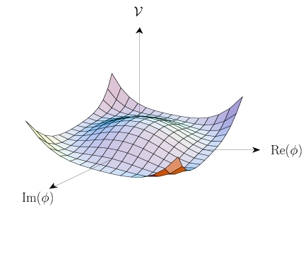
Figure 3.1: Graphical representation of the potential (3.4).

To account for this, we shift $\phi$ by a (complex) constant $\bar{\phi}$ and write

$$\phi(x)={\rm e}^{i\varphi(x)}\,[\bar{\phi}+\tilde{\phi}(x)].$$ (3.5)

The phase field $\varphi(x)$ represents the Goldstone mode accompanying the spontaneous breakdown of the global U(1) symmetry. At zero temperature, the constant value

$$|\bar{\phi}|^{2}=\frac{1}{2}\frac{\mu_{0}}{\lambda_{0}}$$ (3.6)

minimizes the potential energy. It physically represents the number density of particles contained in the condensate for the total particle number density is given by

$$n(x)=|\phi(x)|^{2}.$$ (3.7)

Because $\bar{\phi}$ is a constant, the condensate is a uniform, zero-momentum state. That is, the particles residing in the ground state are in the ${\bf k}=0$ mode. We will be working in the Bogoliubov approximation which amounts to including only the quadratic terms in $\tilde{\phi}$ and ignoring the higher-order ones. These terms may be cast in the matrix form

$${\cal L}^{(2)}={\textstyle\frac{1}{2}}\tilde{\Phi}^{\dagger}M_{0}(p,x)\tilde{\Phi},\;\;\;\;\;\;\tilde{\Phi}=\left(\begin{array}[]{l}\tilde{\phi}\\ \tilde{\phi}^{*}\end{array}\right),$$ (3.8)

with

$$M_{0}(p,x)=$$ (3.12)

$$\!\!\!\!\!\!\!\left(\begin{array}[]{cc}p_{0}-\epsilon({\bf p})+\mu_{0}-U(x)-4\lambda_{0}|\bar{\phi}|^{2}&\!\!\!\!-2\lambda_{0}\bar{\phi}^{2}\\ -2\lambda_{0}\bar{\phi}^{*}\mbox{}^{2}&\!\!\!\!-p_{0}-\epsilon({\bf p})+\mu_{0}-U(x)-4\lambda_{0}|\bar{\phi}|^{2}\end{array}\right),$$

where $U$ stands for the combination

$$U(x)=\partial_{0}\varphi(x)+\frac{1}{2m}[\nabla\varphi(x)]^{2}.$$ (3.13)

In writing (3.12) we have omitted a term $\nabla^{2}\varphi$ containing two derivatives which is irrelevant in the regime of low momentum in which we shall be interested. We also omitted a term of the form $\nabla\varphi\cdot{\bf j}$, where ${\bf j}$ is the Noether current associated with the global U(1) symmetry,

$${\bf j}=\frac{1}{2im}\phi^{*}\stackrel{{\scriptstyle\leftrightarrow}}{{\nabla}}\phi.$$ (3.14)

This term, which after a partial integration becomes $-\varphi\nabla\cdot{\bf j}$, is irrelevant too at low energy and small momentum because in a first approximation the particle number density is constant, so that the classical current satisfies the condition

$$\nabla\cdot{\bf j}=0.$$ (3.15)

The spectrum $E({\bf k})$ obtained from the matrix $M_{0}$ with the field $U$ set to zero is the famous single-particle Bogoliubov spectrum [7],

$$E({\bf k}) = \sqrt{\epsilon^{2}({\bf k})+2\mu_{0}\epsilon({\bf k})}$$ (3.16)

$$= \sqrt{\epsilon^{2}({\bf k})+4\lambda_{0}|\bar{\phi}|^{2}\epsilon({\bf k})}.$$

The most notable feature of this spectrum is that it is gapless, behaving for small momentum as

$$E({\bf k})\sim u_{0}\,|{\bf k}|,$$ (3.17)

with $u_{0}=\sqrt{\mu_{0}/m}$ a velocity which is sometimes referred to as the microscopic sound velocity. It was first shown by Beliaev [8] that the gaplessness of the single-particle spectrum persists at the one-loop order. This was subsequently proven to hold to all orders in perturbation theory by Hugenholtz and Pines [9]. For large momentum, the Bogoliubov spectrum takes a form

$$E({\bf k})\sim\epsilon({\bf k})+2\lambda_{0}|\bar{\phi}|^{2}$$ (3.18)

typical for a nonrelativistic particle with mass $m$ moving in a medium. To highlight the condensate we have chosen here the second form in (3.16) where $\mu_{0}$ is replaced with $2\lambda_{0}|\bar{\phi}|^{2}$.

3.2 Effective Theory

Since gapless modes in general require a justification for their existence, we expect the gaplessness of the single-particle spectrum to be a result of Goldstone’s theorem. This is corroborated by the relativistic version of the theory. There, one finds two spectra, one corresponding to a massive Higgs particle which in the nonrelativistic limit becomes too heavy and decouples from the theory, and one corresponding to the Goldstone mode of the spontaneously broken global U(1) symmetry [10]. The latter reduces in the nonrelativistic limit to the Bogoliubov spectrum. Also, when the theory is coupled to an electromagnetic field, one finds that the single-particle spectrum acquires an energy gap. This is what one expects to happen with the spectrum of a Goldstone mode when the Higgs mechanism is operating. The equivalence of the single-particle excitation and the collective density fluctuation has been proven to all orders in perturbation by Gavoret and Nozières [11].

Let us derive the effective theory governing the Goldstone mode at low energy and small momentum by integrating out the fluctuating field $\tilde{\Phi}$ [12]. The effective theory is graphically represented by Fig. 3.2.

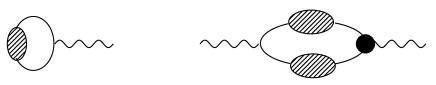
Figure 3.2: Graphical representation of the effective theory (3.25). The symbols are explained in the text.

A line with a shaded bubble inserted stands for $i$ times the full Green function $G$ and the black bubble denotes $i$ times the full interaction $\Gamma$ of the $\tilde{\Phi}$-field with the field $U$ which is denoted by a wiggly line. Both $G$ and $\Gamma$ are $2\times 2$ matrices. The full interaction is obtained from the inverse Green function by differentiation with respect to the chemical potential,

$$\Gamma=-\frac{\partial G^{-1}}{\partial\mu}.$$ (3.19)

This follows because $U$, as defined in (3.13), appears in the theory only in the combination $\mu_{0}-U$. To lowest order, the inverse propagator is given by the matrix $M_{0}$ in (3.12) with $U(x)$ set to zero. It follows that the vertex of the interaction between the $\tilde{\Phi}$ and $U$-fields is minus the unit matrix. Because in terms of the full Green function $G$, the particle number density reads

$$\bar{n}=\frac{i}{2}\,{\rm tr}\int_{k}G(k),$$ (3.20)

we conclude that the first diagram in Fig. 3.2 stands for $-\bar{n}U$. The bar over $n$ is to indicate that the particle number density obtained in this way is a constant, representing the density of the uniform system with $U(x)$ set to zero. The second diagram without the wiggly lines denotes $i$ times the (0 0)-component of the full polarization tensor, $\Pi_{00}$, at zero energy transfer and low momentum ${\bf q}$,

$$i\lim_{{\bf q}\rightarrow 0}\Pi_{00}(0,{\bf q})=-\frac{1}{2}\lim_{{\bf q}\rightarrow 0}{\rm tr}\int_{k}G\,\Gamma\,G\,(k_{0},{\bf k}+{\bf q}).$$ (3.21)

The factor ${\textstyle\frac{1}{2}}$ is a symmetry factor which arises because the two Bose lines are identical. We proceed by invoking an argument due to Gavoret and Nozières [11] to relate the left-hand side of (3.21) to the sound velocity. By virtue of relation (3.19) between the full Green function $G$ and the full interaction $\Gamma$, the (0 0)-component of the polarization tensor can be cast in the form

$$\lim_{{\bf q}\rightarrow 0}\Pi_{00}(0,{\bf q}) = -\frac{i}{2}\lim_{{\bf q}\rightarrow 0}{\rm tr}\int_{k}G\,\frac{\partial G^{-1}}{\partial\mu}\,G(k_{0},{\bf k}+{\bf q})$$ (3.22)

$$= \frac{i}{2}\frac{\partial}{\partial\mu}\lim_{{\bf q}\rightarrow 0}{\rm tr}\int_{k}G(k_{0},{\bf k}+{\bf q})$$

$$= \frac{\partial\bar{n}}{\partial\mu}=-\frac{1}{V}\frac{\partial\Omega}{\partial\mu^{2}},$$

where $\Omega$ is the thermodynamic potential and $V$ the volume of the system. The right-hand side of (3.22) is $\bar{n}^{2}\kappa$, with $\kappa$ the compressibility. Because it is related to the macroscopic sound velocity $c$ via

$$\kappa=\frac{1}{m\bar{n}c^{2}},$$ (3.23)

we conclude that the (0 0)-component of the full polarization tensor satisfies the so-called compressibility sum rule of statistical physics [11]

$$\lim_{{\bf q}\rightarrow 0}\Pi_{00}(0,{\bf q})=\bar{n}^{2}\kappa=\frac{\bar{n}}{mc^{2}}.$$ (3.24)

Putting the pieces together, we infer that the diagrams in Fig. 3.2 stand for the effective theory

$${\cal L}_{{\rm eff}}=-\bar{n}\left[\partial_{0}\varphi+\frac{1}{2m}({\bf\nabla}\varphi)^{2}\right]+\frac{\bar{n}}{2mc^{2}}\left[\partial_{0}\varphi+\frac{1}{2m}({\bf\nabla}\varphi)^{2}\right]^{2},$$ (3.25)

where we recall that ${\bar{n}}$ is the particle number density of the fluid at rest. The theory describes a nonrelativistic sound wave, with the dimensionless phase field $\varphi$ representing the Goldstone mode of the spontaneously broken global U(1) symmetry. It has the gapless dispersion relation $E^{2}({\bf k})=c^{2}{\bf k}^{2}$. The effective theory gives a complete description of the superfluid valid at low energies and small momenta. The same effective theory appears in the context of (neutral) superconductors [13] (see next chapter) and also in that of classical hydrodynamics [14].

The chemical potential $\mu$ is represented in the effective theory (3.25) by [15]

$$\mu(x)=-\partial_{0}\varphi(x),$$ (3.26)

so that

$$\frac{\partial{\cal L}_{\rm eff}}{\partial\mu}=-\frac{\partial{\cal L}_{\rm eff}}{\partial\partial_{0}\phi}=n(x),$$ (3.27)

as required. It also follows from this equation that the particle number density $n(x)$ is canonical conjugate to $-\phi(x)$.

The most remarkable aspect of the effective theory (3.25) is that it is nonlinear. The nonlinearity is necessary to provide a Galilei-invariant description of a gapless mode, as required in a nonrelativistic context. Under a Galilei boosts,

$$t\rightarrow t^{\prime}=t,\;\;{\bf x}\rightarrow{\bf x}^{\prime}={\bf x}-{\bf u}t;\;\;\;\;\partial_{0}\rightarrow\partial_{0}^{\prime}=\partial_{0}+{\bf u}\cdot\nabla,\;\;\nabla\rightarrow\nabla^{\prime}=\nabla,$$ (3.28)

with ${\bf u}$ a constant velocity, the Goldstone field $\varphi(x)$ transforms as

$$\frac{1}{m}\varphi(x)\rightarrow\frac{1}{m}\varphi^{\prime}(x^{\prime})=\frac{1}{m}\varphi(x)-{\bf u}\cdot{\bf x}+{\textstyle\frac{1}{2}}{\bf u}^{2}t.$$ (3.29)

As a result, the superfluid velocity ${\bf v}_{\rm s}=\nabla\varphi/m$ and the chemical potential (per unit mass) $\mu/m=-\partial_{0}\varphi/m$ transform under a Galilei boost in the correct way,

$${\bf v}_{\rm s}(x)\rightarrow{\bf v}^{\prime}_{\rm s}(x^{\prime})={\bf v}_{\rm s}(x)-{\bf u},\;\;\;\mu(x)/m\rightarrow\mu^{\prime}(x^{\prime})/m=\mu(x)/m-{\bf u}\cdot{\bf v}_{\rm s}(x)+{\textstyle\frac{1}{2}}{\bf u}^{2}.$$ (3.30)

It is readily checked that the field $U(x)$ defined in (3.13) and therefore the effective theory (3.25) is invariant under Galilei boosts.

Since the Goldstone field in (3.1) is always accompanied by a derivative, we see that that the nonlinear terms carry additional factors of $|{\bf k}|/mc$, with $|{\bf k}|$ the wave number. They can therefore be ignored provided the wave number is smaller than the inverse coherence length $\xi^{-1}=mc$,

$$|{\bf k}|<1/\xi.$$ (3.31)

For example, in the case of ⁴He the coherence length, or Compton wavelength, is about 10 nm. In this system, the bound (3.31), below which the nonlinear terms can be neglected, coincide with the region where the spectrum is linear and the description in terms of solely a sound mode is applicable.

The alert reader might be worrying about an apparent mismatch in the number of degrees of freedom in the normal and the superfluid phase. Whereas the normal phase is described by a complex $\phi$-field, the superfluid phase is described by a real scalar field $\varphi$. The resolution of this paradox lies in the spectrum of the modes [16]. In the normal phase, the spectrum $E({\bf k})={\bf k}^{2}/2m$ is linear in $E$, so that only positive energies appear in the Fourier decomposition, and one needs—as is well known from standard quantum mechanics—a complex field to describe a single particle. In the superfluid phase, where the spectrum, $E^{2}({\bf k})=c^{2}{\bf k}^{2}$, is quadratic in $E$, the counting goes differently. The Fourier decomposition now contains positive as well as negative energies and a single real field suffice to describe this mode. In other words, although the number of fields is different, the number of degrees of freedom is the same in both phases.

The particle number density and current that follows from (3.25) read

$$n(x) = \bar{n}-\frac{\bar{n}}{mc^{2}}\left\{\partial_{0}\varphi(x)+\frac{1}{2m}[{\bf\nabla}\varphi(x)]^{2}\right\}$$ (3.32)

$${\bf j}(x) = n(x){\bf v}_{\rm s}(x).$$ (3.33)

Physically, (3.32) reflects Bernoulli’s principle which states that in regions of rapid flow, the density and therefore the pressure is low.

The diagrams of Fig. 3.2 can be evaluated in a loop expansion to obtain explicit expressions for the particle number density $\bar{n}$ and the sound velocity $c$ to any given order [12]. In doing so, one encounters—apart from ultraviolet divergences which will be dealt with shortly—also infrared divergences because the Bogoliubov spectrum is gapless. When however all one-loop contributions are added together, these divergences are seen to cancel [12]. One finds for $d=2$ to the one-loop order

$$\bar{n}=\frac{1}{2}\frac{\mu}{\lambda},\;\;\;c^{2}=2\frac{\lambda\bar{n}}{m},$$ (3.34)

where $\mu$ and $\lambda$ are the renormalized parameters. Following Ref. [17], we adopted a dimensional regularization scheme, in which after the integrals over the loop energies have been carried out, the remaining integrals over the loop momenta are analytically continued to arbitrary space dimensions $d$. As renormalization prescription we employed the modified minimal subtraction scheme. This leads to the following relation between the bare ($\lambda_{0}$) and renormalized coupling constant [see Eq. (3.56) below]

$$\frac{1}{\lambda_{0}}=\frac{1}{\kappa^{\epsilon}}\left(\frac{1}{\hat{\lambda}}-\frac{m}{\pi\epsilon}\right),$$ (3.35)

where $\epsilon=2-d$, and $\kappa$ is an arbitrary renormalization group scale parameter introduced to give the renormalized coupling constant $\hat{\lambda}$ the same engineering dimension as in $d=2$. The chemical potential is not renormalized to this order.

Incidentally, from the vantage point of renormalization, the mass $m$ is an irrelevant parameter in nonrelativistic theories and can be scaled away (see, e.g., Ref. [17]).

The form of the effective theory (3.25) can also be derived from general symmetry arguments [18]. More specifically, it follows from making the presence of a gapless Goldstone mode compatible with Galilei invariance which demands that the mass current and the momentum density are equal. The latter observation leads to the conclusion that the U(1) Goldstone field $\varphi$ can only appear in the combination (3.13). To obtain the required linear spectrum for the Goldstone mode it is necessary then to have the form (3.25). Given the form of the effective theory, the particle number density and sound velocity can then more easily be obtained directly from the thermodynamic potential $\Omega$ via

$$\bar{n}=-\frac{1}{V}\frac{\partial\Omega}{\partial\mu};\;\;\;\;\;\;\frac{1}{c^{2}}=-\frac{1}{V}\frac{m}{\bar{n}}\frac{\partial^{2}\Omega}{\partial\mu^{2}},$$ (3.36)

where $V$ is the volume of the system. In this approach, one only has to calculate the thermodynamic potential which at zero temperature and in the Bogoliubov approximation in which we are working is given by the sum ${\cal V}$ of the classical potential ${\cal V}_{0}$ and the effective potential ${\cal V}_{\rm eff}$ corresponding to the theory (3.1):

$$\Omega=\int_{\bf x}({\cal V}_{0}+{\cal V}_{\rm eff}),$$ (3.37)

where ${\cal V}_{0}$ is given by (3.4) with $\phi$ replaced by $\bar{\phi}$. The effective potential for the uniform system is obtained as follows. In the Bogoliubov approximation of ignoring higher than second order in the fields, the integration over $\tilde{\Phi}$ is Gaussian. Carrying out this integral, we obtain for the zero-temperature partition function

$$Z = {\rm e}^{-i\int_{x}{\cal V}_{0}}\int\mbox{D}\phi^{*}\mbox{D}\phi\exp\left(i\int_{x}{\cal L}^{(2)}\right)$$ (3.38)

$$= {\rm e}^{-i\int_{x}{\cal V}_{0}}\,{\rm Det}^{-1/2}(M_{0}),$$

where $M_{0}$ stands for the matrix introduced in (3.12). Setting

$$Z=\exp\left[i\left(-\int_{x}{\cal V}_{0}+S_{\rm eff}\right)\right],$$ (3.39)

we conclude from (3.38) that the effective action in the Bogoliubov approximation is given to the one-loop order by

$$S_{\rm eff}={\textstyle\frac{1}{2}}i{\rm Tr}\ln[M_{0}(p,x)],$$ (3.40)

where we again used the identity Det($A$) = exp[Tr ln($A$)]. The trace Tr appearing here stands besides for the trace over discrete indices now also for the integral $\int_{x}$ over spacetime as well as the one $\int_{k}$ over energy and momentum. The latter integral reflects the fact that the effective action calculated here is a one-loop result with $k_{\mu}$ the loop energy and momentum. To disentangle the integrals one has to carry out similar steps as the ones outlined in Sec. 2.2 and repeatedly apply the identity

$$f(x)p_{\mu}g(x)=(p_{\mu}-i\tilde{\partial}_{\mu})f(x)g(x),$$ (3.41)

where $f(x)$ and $g(x)$ are arbitrary functions of spacetime and the derivative $\tilde{\partial}_{\mu}=(\partial_{0},-\nabla)$ acts only on the next object to the right. The method outlined there can easily be transcribed to the present case where the time dimension is included.

If the field $U(x)$ in $M_{0}$ is set to zero, things simplify because $M_{0}$ now depends on $p_{\mu}$ only. The effective action then becomes $S_{\rm eff}=-\int_{x}{\cal V}_{\rm eff}$ with

$${\cal V}_{\rm eff}=-\frac{i}{2}{\rm tr}\int_{k}\ln[M_{0}(k)]$$ (3.42)

the effective potential. The easiest way to evaluate the integral over the loop variable $k$ is to first differentiate the expression with respect to the chemical potential $\mu_{0}$

$$\frac{\partial}{\partial\mu_{0}}{\rm tr}\,\int_{k}\ln[M_{0}(k)]=-2\,\int_{k}\frac{\epsilon({\bf k})}{k_{0}^{2}-E^{2}({\bf k})+i\eta},$$ (3.43)

with $E({\bf k})$ the Bogoliubov spectrum (3.16). The integral over $k_{0}$ can be carried out with the help of a contour integration, yielding

$$\int_{k}\frac{\epsilon({\bf k})}{k_{0}^{2}-E^{2}({\bf k})+i\eta}=-\frac{i}{2}\,\int_{\bf k}\frac{\epsilon({\bf k})}{E({\bf k})}.$$ (3.44)

This in turn is easily integrated with respect to $\mu_{0}$. Putting the pieces together, we obtain

$${\cal V}=-\frac{\mu_{0}^{2}}{4\lambda_{0}}+\frac{1}{2}\int_{\bf k}E({\bf k}).$$ (3.45)

The integral over the loop momentum in arbitrary space dimension $d$ yields

$${\cal V}=-\frac{\mu_{0}^{2}}{4\lambda_{0}}-L_{d}m^{d/2}\mu_{0}^{d/2+1},\;\;\;L_{d}=\frac{\Gamma(1-d/2)\Gamma(d/2+1/2)}{2\pi^{d/2+1/2}\Gamma(d/2+2)}$$ (3.46)

where we employed the integral representation of the Gamma function

$$\frac{1}{a^{z}}=\frac{1}{\Gamma(z)}\int_{0}^{\infty}\frac{\mbox{d}\tau}{\tau}\tau^{z}{\rm e}^{-a\tau}$$ (3.47)

together with dimensional regularization to suppress irrelevant ultraviolet divergences.

For comparison, let us also evaluate the integral in (3.45) over the loop momentum in three dimensions by introducing a momentum cutoff $\Lambda$

$${\cal V}_{\rm eff}=\frac{1}{2}\int_{\bf k}E({\bf k})=\frac{1}{4\pi^{2}}\int_{0}^{\Lambda}k^{2}E(|{\bf k}|)=$$ (3.48)

$$\frac{1}{4\pi^{2}}\left(\frac{1}{10}\frac{\Lambda^{5}}{m}+\frac{1}{3}\mu_{0}\Lambda^{3}-m\mu_{0}^{2}\Lambda+\frac{32}{15}m^{3/2}\mu_{0}^{5/2}\right)+{\cal O}\left(\frac{1}{\Lambda}\right).$$

From (3.46), we obtain by setting $d=3$ only the finite part, so that all terms diverging with a strictly positive power of the momentum cutoff are suppressed. As we remarked in Sec. 2.2, these contributions, which come from the ultraviolet region, cannot be physically very relevant because the simple model (3.1) breaks down here. On account of the uncertainty principle, stating that large momenta correspond to small distances, these terms are always local and can be absorbed by redefining the parameters appearing in the Lagrangian [19]. Since $\mu_{0}=2\lambda_{0}|\bar{\phi}|^{2}$, we see that the first diverging term in (3.48) is an irrelevant constant, while the two remaining diverging terms can be absorbed by introducing the renormalized parameters

$$\mu = \mu_{0}-\frac{1}{6\pi^{2}}\lambda_{0}\Lambda^{3}$$ (3.49)

$$\lambda = \lambda_{0}-\frac{1}{\pi^{2}}m\lambda_{0}^{2}\Lambda.$$ (3.50)

Because the diverging terms are—at least to this order—of a form already present in the original Lagrangian, the theory is called “renormalizable”. The renormalized parameters are the physical ones that are to be identified with those measured in experiment. In this way, we see that the contributions to the loop integral stemming from the ultraviolet region are of no importance. What remains is the finite part

$${\cal V}_{\rm eff}=\frac{8}{15\pi^{2}}m^{3/2}\mu_{0}^{5/2},$$ (3.51)

which, as we have seen, is obtained directly without renormalization when using dimensional regularization. In this scheme, divergences proportional to powers of the cutoff never show up. Only logarithmic divergences appear as $1/\epsilon$ poles, where $\epsilon$ is the deviation from the upper critical dimension ($d=2$ in the present case). These logarithmic divergences $\ln(\Lambda/E)$, with $E$ an energy scale, are relevant also in the infrared because for fixed cutoff $\ln(\Lambda/E)\rightarrow-\infty$ when $E$ is taken to zero.

In so-called “nonrenormalizable” theories, the ultraviolet-diverging terms are still local but not of a form present in the original Lagrangian. Whereas in former days such theories were rejected because there supposed lack of predictive power, the modern view is that there are no fundamental theories and that there is no basic difference between renormalizable and nonrenormalizable theories [20]. Even a renormalizable theory like (3.1) should be extended to include all higher-order terms such as a $|\phi|^{6}$-term which are allowed by symmetry. These additional terms render the theory “nonrenormalizable”. This does not however change the predictive power of the theory. The point is that when describing the physics at an energy scale $E$ far below the cutoff, the higher-order terms are suppressed by powers of $E/\Lambda$, as follows from dimensional analysis. Therefore, far below the cutoff, the nonrenormalizable terms are negligible.

That $d=2$ is the upper critical dimension of the problem at hand can be seen by noting that $L_{d}$ in (3.46) diverges when $d$ tends to 2. Special care has to be taken for this case. For $d\neq 2$, we obtain with the help of (3.36) [21]

$$\bar{n}=\frac{\mu_{0}}{2\lambda_{0}}\left[1+(d+2)L_{d}m^{d/2}\lambda_{0}\mu_{0}^{d/2-1}\right]$$ (3.52)

and

$$c^{2}=\frac{\mu_{0}}{m}\left[1-(d-2)(d/2+1)L_{d}m^{d/2}\lambda_{0}\mu_{0}^{d/2-1}\right],$$ (3.53)

where to arrive at the last equation an expansion in the coupling constant $\lambda_{0}$ is made. Up to this point, we have considered the chemical potential to be the independent parameter, thereby assuming the presence of a reservoir that can freely exchange particles with the system under study. The system can thus have any number of particles, only the average number is fixed by external conditions. From the experimental point of view it is, however, often more realistic to consider the particle number fixed. If this is the case, the particle number density $\bar{n}$ should be considered as independent variable and the chemical potential should be expressed in terms of it. This can be achieved by inverting relation (3.52):

$$\mu_{0}=2\lambda_{0}\bar{n}\left[1-2(d-2)(d/2+1)L_{d}m^{d/2}\lambda_{0}(2\lambda_{0}\bar{n})^{d/2-1}\right].$$ (3.54)

The sound velocity expressed in terms of the particle number density reads

$$c^{2}=\frac{2\lambda_{0}\bar{n}}{m}\left[1-d(d/2+1)L_{d}m^{d/2}\lambda_{0}(2\lambda_{0}\bar{n})^{d/2-1}\right].$$ (3.55)

These formulas reproduce the known results in $d=3$ [22] and $d=1$ [23].

To investigate the case $d=2$, we expand the potential (3.46) around $d=2$:

$${\cal V}=-\frac{\mu_{0}^{2}}{4\lambda_{0}}-\frac{1}{4\pi\epsilon}\frac{m\mu_{0}^{2}}{\kappa^{\epsilon}}+{\cal O}(\epsilon^{0}),$$ (3.56)

with $\epsilon=2-d$. This expression is seen to diverge in the limit $d\rightarrow 2$. The theory can be rendered finite by introducing a renormalized coupling constant via (3.35). We also see that the chemical potential is not renormalized to this order. The beta function $\beta(\hat{\lambda})$ follows as [24]

$$\beta(\hat{\lambda})=\kappa\left.\frac{\partial\hat{\lambda}}{\partial\kappa}\right|_{\lambda_{0}}=-\epsilon\hat{\lambda}+\frac{m}{\pi}\hat{\lambda}^{2}.$$ (3.57)

In the upper critical dimension, this yields only one fixed point, viz. the infrared-stable (IR) fixed point $\hat{\lambda}^{*}=0$. Below $d=2$, this point is shifted to $\hat{\lambda}^{*}=\epsilon\pi/m$. It is now easily checked that Eqs. (3.52) and (3.55) also reproduce the two-dimensional results (3.34).

In the one-loop approximation there is no field renormalization; this is the reason why in (3.1) we gave only the bare parameters $\mu_{0}$ and $\lambda_{0}$ an index 0, and not $\phi$.

We proceed by calculating the fraction of particles residing in the condensate. In deriving the Bogoliubov spectrum (3.16), we set $|\bar{\phi}|^{2}=\mu_{0}/2\lambda_{0}$ thereby fixing the number density of particles contained in the condensate,

$$\bar{n}_{0}=|\bar{\phi}|^{2},$$ (3.58)

in terms of the chemical potential. For our present consideration we have to keep $\bar{\phi}$ as independent variable. The spectrum of the elementary excitation expressed in terms of $\bar{\phi}$ is

$$E({\bf k})=\sqrt{\bigl{[}\epsilon({\bf k})-\mu_{0}+4\lambda_{0}|\bar{\phi}|^{2}\bigr{]}^{2}-4\lambda_{0}^{2}|\bar{\phi}|^{4}}\,.$$ (3.59)

It reduces to the Bogoliubov spectrum when the mean-field value (3.6) for $\bar{\phi}$ is inserted. Equation (3.42) for the effective potential is still valid, and so is (3.37). We thus obtain for the particle number density

$$\bar{n}=\left.|\bar{\phi}|^{2}-\frac{1}{2}\frac{\partial}{\partial\mu_{0}}\int_{\bf k}E({\bf k})\right|_{|\bar{\phi}|^{2}=\mu_{0}/2\lambda_{0}},$$ (3.60)

where the mean-field value for $\bar{\phi}$ is to be substituted after the differentiation with respect to the chemical potential has been carried out. We find

$$\bar{n}=|\bar{\phi}|^{2}-2^{d/2-2}\frac{d^{2}-4}{d-1}L_{d}m^{d/2}\lambda_{0}^{d/2}|\bar{\phi}|^{d}$$ (3.61)

or for the so-called depletion of the condensate [25]

$$\frac{\bar{n}}{\bar{n}_{0}}-1\approx-2^{d/2-2}\frac{d^{2}-4}{d-1}L_{d}m^{d/2}\lambda^{d/2}n^{d/2-1},$$ (3.62)

where in the last term we replaced the bare coupling constant with the (one-loop) renormalized one. This is consistent to this order since this term is already a one-loop result. Equation (3.62) shows that even at zero temperature not all the particles reside in the condensate. Due to the interparticle repulsion, particles are removed from the zero-momentum ground state and put in states of finite momentum. It has been estimated that in bulk superfluid ⁴He—a strongly interacting system—only about 8% of the particles condense in the zero-momentum state [26]. For $d=2$, the right-hand side of Eq. (3.62) reduces to

$$\frac{\bar{n}}{\bar{n}_{0}}-1\approx\frac{m\lambda}{2\pi},$$ (3.63)

which is seen to be independent of the particle number density.

Despite the fact that not all the particles reside in the condensate, they all participate in the superfluid motion at zero temperature [27]. Apparently, the condensate drags the normal fluid along with it. To show this, let us assume that the entire system moves with a velocity ${\bf u}$ relative to the laboratory system. As is known from standard hydrodynamics the time derivate in the frame following the motion of the fluid is $\partial_{0}+{\bf u}\cdot\nabla$ [see Eq. (3.28)]. If we insert this in the Lagrangian (3.1) of the interacting Bose gas, it becomes

$${\cal L}=\phi^{*}[i\partial_{0}-\epsilon(-i\nabla)+\mu_{0}-{\bf u}\cdot(-i\nabla)]\phi-\lambda_{0}|\phi|^{4},$$ (3.64)

where the extra term features the total momentum $\int_{\bf x}\phi^{*}(-i\nabla)\phi$ of the system. The velocity $-{\bf u}$ multiplying this is on the same footing as the chemical potential $\mu_{0}$ multiplying the particle number $\int_{\bf x}|\phi|^{2}$. Whereas $\mu_{0}$ is associated with particle number conservation, ${\bf u}$ is related to the conservation of momentum.

In the two-fluid picture, the condensate can move with a different velocity ${\bf v}_{\rm s}$ as the rest of the system. To bring this out we introduce new fields, cf. (3.5)

$$\phi(x)\rightarrow\phi^{\prime}(x)={\rm e}^{im{\bf v}_{\rm s}\cdot{\bf x}}\phi(x)$$ (3.65)

in terms of which the Lagrangian becomes [28]

$${\cal L}=\phi^{*}\bigl{[}i\partial_{0}-\epsilon(-i\nabla)+\mu_{0}-{\textstyle\frac{1}{2}}m{\bf v}_{\rm s}\cdot({\bf v}_{\rm s}-2{\bf u})-({\bf u}-{\bf v}_{\rm s})\cdot(-i\nabla)\bigr{]}\phi-\lambda_{0}|\phi|^{4},$$ (3.66)

where we dropped the primes on $\phi$ again. Both velocities appear in this expression. Apart from the change ${\bf u}\rightarrow{\bf u}-{\bf v}_{\rm s}$ in the second last term, the field transformation resulted in a change of the chemical potential

$$\mu_{0}\rightarrow\mu_{\rm eff}:=\mu_{0}-{\textstyle\frac{1}{2}}m{\bf v}_{\rm s}\cdot({\bf v}_{\rm s}-2{\bf u})$$ (3.67)

where $\mu_{\rm eff}$ may be considered as an effective chemical potential.

The equations for the Bogoliubov spectrum and the thermodynamic potential are readily written down for the present case with these two changes are kept in mind. In particular, the effective potential is given by (3.45) with the replacement Eq. (3.67). The momentum density, or equivalently, the mass current ${\bf g}$ of the system is obtained in this approximation by differentiating the effective potential with respect to $-{\bf u}$. We find, using the equation

$$\frac{\partial\mu_{\rm eff}}{\partial{\bf u}}=m{\bf v}_{\rm s}$$ (3.68)

that it is given by

$${\bf g}=\rho_{\rm s}{\bf v}_{\rm s},$$ (3.69)

with $\rho_{\rm s}=m\bar{n}$ the superfluid mass density. This equation, comprising the total particle number density $\bar{n}$, shows that at zero temperature indeed all the particles are involved in the superflow, despite the fact that only a fraction of them resides in the condensate [27]. The superfluid mass density $\rho_{\rm s}$, obtained by evaluating the response of the system to an externally imposed velocity field ${\bf u}$, should not be confused with the number density $\bar{n}_{0}$ of particles contained in the condensate introduced in Eq. (3.58).

Let us close this section by pointing out a quick trail to arrive at the effective theory (3.25) starting from the microscopic model (3.1). To this end we set

$$\phi(x)={\rm e}^{i\varphi(x)}\,[\sqrt{\bar{n}}+\tilde{\phi}(x)],$$ (3.70)

and expand the Lagrangian (3.1) up to quadratic terms in $\tilde{\phi}$. This leads to

$${\cal L}^{(2)}=-{\cal V}_{0}-\bar{n}U-\sqrt{\bar{n}}U(\tilde{\phi}+\tilde{\phi}^{*})-\lambda_{0}\bar{n}(\tilde{\phi}+\tilde{\phi}^{*})^{2},$$ (3.71)

where we used the mean-field equation $\mu_{0}=2\lambda_{0}\bar{n}$. We next integrate out the tilde fields—which is tantamount to substituting the field equation for these fields back into the Lagrangian—to obtain

$${\cal L}_{\rm eff}=-\bar{n}U(x)+\frac{1}{4}U(x)\frac{1}{\lambda_{0}}U(x),$$ (3.72)

apart from the irrelevant constant term ${\cal V}_{0}$. This form of the effective theory is equivalent to the one found before in (3.1). We have cast the last term in a form that can be easily generalized to systems with long-ranged interactions. A case of particular interest to us is the Coulomb potential

$$V({\bf x})=\frac{e_{0}^{2}}{|{\bf x}|},$$ (3.73)

whose Fourier transform in $d$ space dimensions reads

$$V({\bf k})=2^{d-1}\pi^{(d-1)/2}\Gamma\left[{\textstyle\frac{1}{2}}(d-1)\right]\frac{e_{0}^{2}}{|{\bf k}|^{d-1}}.$$ (3.74)

The simple contact interaction $L_{\rm i}=-\lambda_{0}\int_{\bf x}|\phi(x)|^{4}$ in (3.1) gets now replaced by

$$L_{\rm i}=-\frac{1}{2}\int_{{\bf x},{\bf y}}|\phi(t,{\bf x})|^{2}V({\bf x}-{\bf y})|\phi(t,{\bf y})|^{2}.$$ (3.75)

The rationale for using the three-dimensional Coulomb potential even when considering charges confined to move in a lower dimensional space is that the electromagnetic interaction remains three-dimensional. The effective theory (3.72) now becomes in the Fourier representation

$${\cal L}_{\rm eff}=-\bar{n}U(k)+\frac{1}{2}U(k_{0},{\bf k})\frac{1}{V({\bf k})}U(k_{0},-{\bf k})$$ (3.76)

and leads to the dispersion relation

$$E^{2}({\bf k})=2^{d}\pi^{(d-1)/2}\Gamma\left[{\textstyle\frac{1}{2}}(d-1)\right]\frac{\bar{n}e_{0}^{2}}{m}|{\bf k}|^{3-d}.$$ (3.77)

For $d=3$, this yields the famous plasma mode with an energy gap given by the plasma frequency $\omega_{\rm p}^{2}=4\pi\bar{n}e_{0}^{2}/m$.

To appreciate under which circumstances the Coulomb interaction becomes important, we note that for electronic systems $1/|{\bf x}|\sim k_{\rm F}$ for dimensional reasons and the fermion number density $\bar{n}\sim k_{\rm F}^{d}$, where $k_{\rm F}$ is the Fermi momentum. The ratio of the Coulomb interaction energy $\epsilon_{\rm C}$ to the Fermi energy $\epsilon_{\rm F}=k_{\rm F}^{2}/2m$ is therefore proportional to $\bar{n}^{-1/d}$. This means that the lower the electron number density, the more important the Coulomb interaction becomes.

3.3 Quenched Impurities

In most of the quantum systems we will be considering, impurities plays an important role. The main effect of impurities is typically to localize states. Localization counteracts the tendency of the system to become superfluid. We shall therefore now include impurities in the interacting Bose gas to see whether this leads to localization and whether the system still has a superfluid phase. It is expected that on increasing the strength of the disorder for a given repulsive interparticle interaction, the superfluid undergoes a zero-temperature phase transition to an insulating phase of localized states. The location and nature of this transition will be the subject of Ch. 6.

We shall assume that the impurities are fixed and that their distribution is not affected by the host system. This type of impurities is called quenched impurities and is to be distinguished from so-called annealed impurities which change with and depend on the host system. To account for impurities, we add to the theory (3.1) the term

$${\cal L}_{\Delta}=\psi({\bf x})\,|\phi(x)|^{2},$$ (3.78)

with $\psi({\bf x})$ a random field whose distribution is assumed to be Gaussian [29]

$$P(\psi)=\exp\left[-\frac{1}{\Delta_{0}}\int_{\bf x}\,\psi^{2}({\bf x})\right],$$ (3.79)

and characterized by the disorder strength $\Delta_{0}$. The engineering dimension of the random field is the same as that of the chemical potential which is one, $[\psi]=1$, while that of the parameter $\Delta_{0}$ is $[\Delta_{0}]=2-d$ so that the exponent in (3.79) is dimensionless. Since $\psi({\bf x})$ depends only on the $d$ spatial dimensions, the impurities it describes should be considered as grains randomly distributed in space. The quantity

$$Z[\psi]=\int\mbox{D}\phi^{*}\mbox{D}\phi\,\exp\left(i\int_{x}\,{\cal L}\right),$$ (3.80)

where now ${\cal L}$ stands for the Lagrangian (3.1) with the term (3.78) added, is the zero-temperature partition function for a given impurity configuration $\psi$. In the case of quenched impurities, the average of an observable $O(\phi^{*},\phi)$ is obtained as follows

$$\langle O(\phi^{*},\phi)\rangle=\int\mbox{D}\psi P(\psi)\langle O(\phi^{*},\phi)\rangle_{\psi},$$ (3.81)

where $\langle O(\phi^{*},\phi)\rangle_{\psi}$ indicates the grand-canonical average for a given impurity configuration. In other words, first the ensemble average is taken, and only after that the averaging over the random field is carried out.

In terms of the shifted field, the added term reads

$${\cal L}_{\Delta}=\psi({\bf x})(|\bar{\phi}|^{2}+|\tilde{\phi}|^{2}+\bar{\phi}\tilde{\phi}^{*}+\bar{\phi}^{*}\tilde{\phi}).$$ (3.82)

The first two terms lead to an irrelevant change in the chemical potential, so that we only have to consider the last two terms, which we can cast in the form

$${\cal L}_{\Delta}=\psi({\bf x})\,\bar{\Phi}^{\dagger}\tilde{\Phi},\;\;\;\;\;\;\;\bar{\Phi}=\left(\begin{array}[]{l}\bar{\phi}\\ \bar{\phi}^{*}\end{array}\right).$$ (3.83)

The integral over $\tilde{\Phi}$ is Gaussian in the Bogoliubov approximation and is easily performed to yield an additional term to the effective action

$$S_{\Delta}=-\frac{1}{2}\int_{x,y}\psi({\bf x})\bar{\Phi}^{\dagger}\,G_{0}(x-y)\bar{\Phi}\psi({\bf y}),$$ (3.84)

where the propagator $G_{0}$ is the inverse of the matrix $M_{0}$ introduced in (3.12) with the field $U(x)$ set to zero. Let us first Fourier transform the fields,

$$G_{0}(x-y) = \int_{k}{\rm e}^{-ik\cdot(x-y)}\,G_{0}(k)$$ (3.85)

$$\psi({\bf x}) = \int_{\bf k}{\rm e}^{i{\bf k}\cdot{\bf x}}\psi({\bf k}).$$ (3.86)

The contribution to the effective action then appears in the form

$$S_{\Delta}=-\frac{1}{2}\int_{\bf k}|\psi({\bf k})|^{2}\bar{\Phi}^{\dagger}G(0,{\bf k})\bar{\Phi}.$$ (3.87)

Since the random field is Gaussian distributed [see (3.79)], the average over this field representing quenched impurities yields,

$$\langle|\psi({\bf k})|^{2}\rangle={\textstyle\frac{1}{2}}V\Delta_{0}.$$ (3.88)

The remaining integral over the loop momentum in (3.87) is readily carried out to yield

$$\langle{\cal L}_{\Delta}\rangle=\frac{1}{2}\Gamma(1-d/2)\left(\frac{m}{2\pi}\right)^{d/2}|\bar{\phi}|^{2}(6\lambda_{0}|\bar{\phi}|^{2}-\mu_{0})^{d/2-1}\Delta_{0}.$$ (3.89)

This contribution is seen to diverge in the limit $d\rightarrow 2$:

$$\langle{\cal L}_{\Delta}\rangle=\frac{1}{4\pi}\frac{m\mu_{0}}{\lambda_{0}\kappa^{\epsilon}}\frac{\Delta_{0}}{\epsilon},$$ (3.90)

where we substituted the mean-field value $\mu_{0}=2\lambda_{0}|\bar{\phi}|^{2}$. Recall that $\kappa$ is an arbitrary scale parameter introduced for dimensional reasons; the engineering dimension of the right-hand side in (3.90) has the correct value $3-\epsilon$ this way. The result (3.90) is a first indication of the importance of impurities in $d=2$, showing that in order to render the random theory finite a modified renormalized coupling constant $\hat{\lambda}$ has to be introduced via, cf. (3.35),

$$\frac{1}{\lambda_{0}}=\frac{1}{\kappa^{\epsilon}}\left[\frac{1}{\hat{\lambda}}-\frac{m}{\pi\epsilon}\left(1-\frac{\hat{\Delta}}{\mu\hat{\lambda}}\right)\right],$$ (3.91)

which depends on the disorder strength. The renormalized parameter $\hat{\Delta}$ is defined in the same way as $\hat{\lambda}$.

In the previous section we saw that due to the interparticle repulsion, not all the particles reside in the condensate. We expect that the random field causes an additional depletion of the condensate. To obtain this, we differentiate (3.89) with respect to the chemical potential. This gives [30]

$$\bar{n}_{\Delta}=\frac{\partial{\langle\cal L}_{\Delta}\rangle}{\partial\mu}=\frac{2^{d/2-5}\Gamma(2-d/2)}{\pi^{d/2}}m^{d/2}\lambda^{d/2-2}\bar{n}_{0}^{d/2-1}\Delta,$$ (3.92)

where $\bar{n}_{0}$ denotes the density of particles residing in the condensate. We have here again replaced the bare parameters with the (one-loop) renormalized ones. This is consistent to this order since (3.92) is already a one-loop result.

The divergence in the limit $\lambda\rightarrow 0$ for $d<4$ signals the collapse of the system when the interparticle repulsion is removed. Note that in $d=2$, the depletion is independent of the condensate density $\bar{n}_{0}$ [31]:

$$\bar{n}_{\Delta}=\frac{1}{16\pi}\frac{m}{\lambda}\Delta.$$ (3.93)

The total particle number density $\bar{n}$ is given by

$$\bar{n}=\bar{n}_{0}\left(1+\frac{m\lambda}{2\pi}\right)+\frac{1}{16\pi}\frac{m}{\lambda}\Delta.$$ (3.94)

We next calculate the mass current ${\bf g}$ to determine the superfluid mass density, i.e., the mass density flowing with the superfluid velocity ${\bf v}_{\rm s}$. As we have seen in the preceding section, in the absence of impurities and at zero temperature all the particles participate in the superflow and move on the average with the velocity ${\bf v}_{\rm s}$. We expect this to no longer hold in the presence of impurities. To determine the change in the superfluid mass density due to impurities, we replace $\mu_{0}$ with $\mu_{\rm eff}$ as defined in (3.67) and $i\partial_{0}$ with $i\partial_{0}-({\bf u}-{\bf v}_{\rm s})\cdot(-i\nabla)$ in the contribution (3.87) to the effective action, and differentiate it with respect to $-{\bf u}$—the externally imposed velocity. We find to linear order in the difference ${\bf u}-{\bf v}_{\rm s}$:

$${\bf g}=\rho_{\rm s}{\bf v}_{\rm s}+\rho_{\rm n}{\bf u},$$ (3.95)

with the superfluid and normal mass density [30]

$$\rho_{\rm s}=m\left(\bar{n}-\frac{4}{d}\bar{n}_{\Delta}\right),\;\;\;\;\rho_{\rm n}=\frac{4}{d}m\bar{n}_{\Delta}.$$ (3.96)

We see that the normal density is a factor $4/d$ larger than the mass density $m\bar{n}_{\Delta}$ knocked out of the condensate by the impurities. (For $d=3$ this gives the factor ${\textstyle\frac{4}{3}}$ first found in Ref. [32].) Apparently, part of the zero-momentum states belongs for $d<4$ not to the condensate, but to the normal fluid. Being trapped by the impurities, this fraction of the zero-momentum states are localized. This shows that the phenomenon of localization can be accounted for in the Bogoliubov theory of superfluidity by including a random field.

3.4 Vortices

We shall now include vortices in the system. A vortex in two space dimensions may be pictured as a point-like object at scales large compared to their core seize. It is characterized by the winding number $w$ of the map

$$\varphi({\bf x}):{\rm S}^{1}_{\bf x}\rightarrow{\rm S}^{1}$$ (3.97)

of a circle S${}^{1}_{\bf x}$ around the vortex into the internal circle S¹ parameterized by the Goldstone field $\varphi$. In the microscopic theory (3.1), the asymptotic solution of a static vortex with winding number $w$ located at the origin is well known [33]

$$\phi({\bf x})=\sqrt{\frac{\mu_{0}}{2\lambda_{0}}}\left(1-\xi_{0}^{2}\frac{w^{2}}{4{\bf x}^{2}}\right){\rm e}^{iw\theta}+{\cal O}\left(\frac{1}{{\bf x}^{4}}\right),$$ (3.98)

where $\theta$ is the azimuthal angle and $\xi_{0}=1/\sqrt{m\mu_{0}}=1/mc_{0}$ is the coherence length. The density profile $n({\bf x})$ in the presence of this vortex follows from taking $|\phi({\bf x})|^{2}$.

To incorporate vortices in the effective theory we employ the powerful principle of defect gauge symmetry developed by Kleinert [34, 35, 36]. In this approach, one introduces a so-called vortex gauge field $\varphi_{\mu}^{\rm P}=(\varphi_{0}^{\rm P},\mbox{\boldmath$\varphi$}^{\rm P})$ in the effective theory (3.25) via minimally coupling to the Goldstone field:

$$\tilde{\partial}_{\mu}\varphi\rightarrow\tilde{\partial}_{\mu}\varphi+\varphi_{\mu}^{\rm P},$$ (3.99)

with $\tilde{\partial}_{\mu}=(\partial_{0},-\nabla)$. If there are $N$ vortices with winding number $w_{\alpha}$ ($\alpha=1,\cdots,N$) centered at ${\bf X}^{1}(t),\cdots,{\bf X}^{N}(t)$, the plastic field satisfies the relation

$$\nabla\times\mbox{\boldmath$\varphi$}^{\rm P}(x)=-2\pi\sum_{\alpha}w_{\alpha}\delta[{\bf x}-{\bf X}^{\alpha}(t)],$$ (3.100)

so that we obtain for the superfluid velocity field

$$\nabla\times{\bf v}_{\rm s}=\sum_{\alpha}\gamma_{\alpha}\delta[{\bf x}-{\bf X}^{\alpha}(t)],$$ (3.101)

as required. Here, $\gamma_{\alpha}=(2\pi/m)w_{\alpha}$ is the circulation of the $\alpha$th vortex which is quantized in units of $2\pi/m$. A summation over the indices labeling the vortices will always be made explicit. The combination $\tilde{\partial}_{\mu}\varphi+\varphi_{\mu}^{\rm P}$ is invariant under the local gauge transformation

$$\varphi(x)\rightarrow\varphi(x)+\alpha(x);\;\;\;\;\;\varphi^{\rm P}_{\mu}\rightarrow\varphi^{\rm P}_{\mu}-\tilde{\partial}_{\mu}\alpha(x),$$ (3.102)

with $\varphi^{\rm P}_{\mu}$ playing the role of a gauge field.

In the gauge $\varphi^{\rm P}_{0}=0$, Eq. (3.100) can be solved to yield

$$\varphi^{\rm P}_{i}(x)=2\pi\epsilon_{ij}\sum_{\alpha}w_{\alpha}\delta_{j}[x,L_{\alpha}(t)]$$ (3.103)

where $\epsilon_{ij}$ is the antisymmetric Levi-Civita symbol in two dimensions, with $\epsilon_{12}=1$, and $\mbox{\boldmath$\delta$}[x,L_{\alpha}(t)]$ is a delta function on the line $L_{\alpha}(t)$ starting at the center ${\bf X}^{\alpha}(t)$ of the $\alpha$th vortex and running to spatial infinity along an arbitrary path:

$$\delta_{i}[x,L_{\alpha}(t)]=\int_{L_{\alpha}(t)}\mbox{d}y_{i}\,\delta({\bf x}-{\bf y}).$$ (3.104)

Let us for the moment concentrate on static vortices. The field equation obtained from the effective theory (3.25) with $\nabla\varphi$ replaced by the covariant derivative $\nabla\varphi-\mbox{\boldmath$\varphi$}^{\rm P}$ and $\partial_{0}\varphi$ set to zero simply reads

$$\nabla\cdot{\bf v}_{\rm s}=0,\;\;\;\;{\rm or}\;\;\;\;\nabla\cdot(\nabla\varphi-\mbox{\boldmath$\varphi$}^{\rm P})=0,$$ (3.105)

when the fourth-order term is neglected. It can be easily solved to yield

$$\varphi({\bf x})=-\int_{\bf y}G({\bf x}-{\bf y})\nabla\cdot\mbox{\boldmath$\varphi$}^{\rm P}({\bf y}),$$ (3.106)

where $G({\bf x})$ is the Green function of the Laplace operator

$$G({\bf x})=\int_{\bf k}\frac{{\rm e}^{i{\bf k}\cdot{\bf x}}}{{\bf k}^{2}}=-\frac{1}{2\pi}\ln(|{\bf x}|).$$ (3.107)

For the velocity field we obtain in this way the well-known expression [37]

$$v_{i}({\bf x})=\frac{1}{2\pi}\epsilon_{ij}\sum_{\alpha=1}^{N}\gamma_{\alpha}\frac{x_{j}-X^{\alpha}_{j}}{|{\bf x}-{\bf X}^{\alpha}|^{2}},$$ (3.108)

which is valid for ${\bf x}$ sufficiently far away from the vortex cores. Let us now specialize to the case of a single static vortex at the origin. On substituting the corresponding solution in (3.32), we find for the density profile in the presence of a static vortex asymptotically

$$n({\bf x})=\bar{n}\left(1-\xi_{0}^{2}\frac{w^{2}}{2{\bf x}^{2}}\right).$$ (3.109)

This is the same formula as the one obtained from the solution (3.98) of the microscopic theory. This exemplifies that with the aid of the defect gauge symmetry principle, vortices are correctly accounted for in the effective theory.

Let us proceed to investigate the dynamics of vortices in this formalism and derive the action which governs it. We consider only the first part of the effective theory (3.25). In ignoring the higher-order terms, we approximate the superfluid by an incompressible fluid for which the particle number density is constant, $n(x)=\bar{n}$, see Eq. (3.32). We again work in the gauge $\varphi^{\rm P}_{0}=0$ and replace $\nabla\varphi$ by the covariant derivative $\nabla\varphi-\mbox{\boldmath$\varphi$}^{\rm P}$, with the plastic field given by (3.100). The solution of the resulting field equation for $\varphi$ is again of the form (3.106), but now it is time-dependent because the plastic field is. Substituting this in the action $S_{\rm eff}=\int_{x}{\cal L}_{\rm eff}$, we find after some straightforward calculus

$$S_{\rm eff}=m\bar{n}\int_{t}\left[\frac{1}{2}\sum_{\alpha}\gamma_{\alpha}{\bf X}^{\alpha}\times\dot{\bf X}^{\alpha}+\frac{1}{2\pi}\sum_{\alpha<\beta}\gamma_{\alpha}\gamma_{\beta}\ln(|{\bf X}^{\alpha}-{\bf X}^{\beta}|/a)\right].$$ (3.110)

The constant $a$ has the dimension of a length and is included in the argument of the logarithm for dimensional reasons. Physically, it represents the core size of a vortex. The first term in (3.110) leads to a twisted canonical structure which is reminiscent of that found in the so-called Landau problem of a charged particle confined to move in a plane perpendicular to an applied magnetic field $H$.

To display the canonical structure, let us rewrite the first term of the Lagrangian corresponding to (3.110) as

$$L_{1}=m\bar{n}\sum_{\alpha}\gamma_{\alpha}X^{\alpha}_{1}\dot{X}^{\alpha}_{2},$$ (3.111)

where we ignored a total derivative. It follows that the canonical conjugate to the second component $X_{2}^{\alpha}$ of the center coordinate ${\bf X}^{\alpha}$ is essentially its first component [38]

$$\frac{\partial L_{1}}{\partial\dot{X}_{2}^{\alpha}}=m\bar{n}\gamma_{\alpha}X^{\alpha}_{1}.$$ (3.112)

It implies that phase space coincides with real space and gives rise to the commutation relation

$$[X_{2}^{\alpha},X_{1}^{\beta}]=\frac{i}{w_{\alpha}}\ell^{2}\delta^{\alpha\beta},$$ (3.113)

where

$$\ell=1/\sqrt{2\pi\bar{n}}$$ (3.114)

is a characteristic length whose definition is such that $2\pi\ell^{2}$ is the average area occupied by a particle of the superfluid film. The commutation relation leads to an uncertainty in the location of the vortex centers given by

$$\Delta X_{1}^{\alpha}\Delta X_{2}^{\alpha}\geq\frac{\ell^{2}}{2|w_{\alpha}|},$$ (3.115)

which is inverse proportional to the particle number density.

From elementary quantum mechanics we know that to each unit cell (of area $h$) in phase space there corresponds one quantum state. That is, the number of states in an area $S$ of phase space is given by

$$\mbox{\# states in}\;S=\frac{1}{h}\int_{S}\mbox{d}p\,\mbox{d}q,$$ (3.116)

where $p$ and $q$ are a pair of canonically conjugate variables. For the case at hand, this implies that the available number of states in an area $S_{\alpha}$ of real space is

$$\mbox{\# states in}\;S_{\alpha}=|w_{\alpha}|\,\bar{n}S_{\alpha},$$ (3.117)

or, equivalently, that the number of states per unit area available to the $\alpha$th vortex is $|w_{\alpha}|\,\bar{n}$.

This phenomenon that phase space coincides with real space is known to also arise in the Landau problem. There, it leads to the well-known degeneracy $|e_{\alpha}|H/h$ of each Landau level, where $e_{\alpha}=v_{\alpha}e_{0}$ is the electric charge of the particle, with $e_{0}(>0)$ the unit of charge. In terms of the magnetic flux quantum $\Phi_{0}=h/e_{0}$, the Landau degeneracy can be rewritten as $|v_{\alpha}|H/\Phi_{0}=|v_{\alpha}|\bar{n}_{\otimes}$, with $\bar{n}_{\otimes}$ the flux number density. In other words, whereas the degeneracy in the case of vortices in a superfluid film is given by the particle number density, here it is given by the flux number density. Using this analogy, we see that the characteristic length (3.114) translates into $\ell_{H}=1/\sqrt{2\pi\bar{n}_{\otimes}}$ which is precisely the magnetic length of the Landau problem.

The first term in the action (3.110) is also responsible for the so-called geometrical phase [39] acquired by the wavefunction of a vortex when it traverses a closed path. Let us first discuss the case of a charged particle moving adiabatically around a close path $\Gamma_{\alpha}$. Its wavefunction picks up an extra Aharonov-Bohm phase factor given by the Wilson loop:

$$W(\Gamma_{\alpha})=\exp[i\gamma(\Gamma_{\alpha})]=\exp\left(\frac{ie_{\alpha}}{\hbar}\oint_{\Gamma_{\alpha}}\mbox{d}{\bf x}\cdot{\bf A}\right)=\exp\left[2\pi iv_{\alpha}\frac{HS(\Gamma_{\alpha})}{\Phi_{0}}\right]$$ (3.118)

where ${\bf A}$ is the vector potential describing the external magnetic field and $HS(\Gamma_{\alpha})$ is the magnetic flux through the area $S(\Gamma_{\alpha})$ spanned by the loop $\Gamma_{\alpha}$. The geometrical phase $\gamma(\Gamma_{\alpha})$ in (3.118) is seen to be ($2\pi v_{\alpha}$ times) the number of flux quanta enclosed by the path $\Gamma_{\alpha}$.

On account of the above analogy, it follows that the geometrical phase picked up by the wavefunction of a vortex when it is moved adiabatically around a closed path in the superfluid film is ($2\pi w_{\alpha}$ times) the number of superfluid particles enclosed by the path [40].

The second term in the action (3.110) represents the long-ranged interaction between two vortices mediated by the exchange of Goldstone quanta. The action yields the well-known equations of motion for point vortices in an incompressible two-dimensional superfluid [37, 41]:

$$\dot{X}_{i}^{\beta}(t)=\frac{\epsilon_{ij}}{2\pi}\sum_{\alpha\neq\beta}\gamma_{\alpha}\frac{X^{\beta}_{j}(t)-X^{\alpha}_{j}(t)}{|{\bf X}^{\beta}(t)-{\bf X}^{\alpha}(t)|^{2}}.$$ (3.119)

Note that $\dot{X}_{i}^{\beta}(t)=v_{i}\left[{\bf X}^{\beta}(t)\right]$, where ${\bf v}(x)$ is the superfluid velocity (3.108) with the time-dependence of the centers of the vortices included. This nicely illustrates a result due to Helmholtz for ideal fluids, stating that a vortex moves with the fluid, i.e., at the local velocity produced by the other vortices in the system. Experimental support for this conclusion has been reported in Ref. [42].

3.5 Kosterlitz-Thouless Phase Transition

Although we are interested mainly in quantum phase transitions in these Lectures, there is one classical phase transition special to two dimensions which turns out to be relevant for our discussion later on—the so-called Kosterlitz-Thouless phase transition. It is well known that a superfluid film undergoes such a phase transition at a temperature well below the bulk transition temperature. The superfluid low-temperature state is characterized by tightly bound vortex-antivortex pairs which at the Kosterlitz-Thouless temperature unbind and thereby disorder the superfluid state. The disordered state, at temperatures still below the bulk transition temperature, consists of a plasma of unbound vortices.

Since the phase transition is an equilibrium transition, we can ignore any time dependence. The important fluctuations here, at temperatures below the bulk transition temperature, are phase fluctuations so that we can consider the London limit, where the phase of the $\phi(x)$-field is allowed to vary in spacetime while the modulus is kept fixed, and take as Hamiltonian

$${\cal H}={\textstyle\frac{1}{2}}\rho_{\rm s}{\bf v}^{2}_{\rm s},$$ (3.120)

where $\rho_{\rm s}$ is the superfluid mass density which we assume to be constant and ${\bf v}_{\rm s}$ is the superfluid velocity

$${\bf v}_{\rm s}=\frac{1}{m}(\nabla\varphi-\mbox{\boldmath$\varphi$}^{\rm P}),$$ (3.121)

with the vortex gauge field $\mbox{\boldmath$\varphi$}^{\rm P}$ included to account for possible vortices in the system. We shall restrict ourselves to vortices of unit winding number, so that $w_{\alpha}=\pm 1$ for a vortex and antivortex, respectively.

The canonical partition function describing the equilibrium configuration of $N_{+}$ vortices and $N_{-}$ antivortices in a superfluid film is given by

$$Z_{N}=\frac{1}{N_{+}!N_{-}!}\prod_{\alpha}\int_{{\bf X}^{\alpha}}\int\mbox{D}\varphi\,\exp\left(-\beta\int_{\bf x}{\cal H}\right),$$ (3.122)

with ${\cal H}$ the Hamiltonian (3.120) and $N=N_{+}+N_{-}$ the total number of vortices and antivortices. The factors $N_{+}!$ and $N_{-}!$ arise because the vortices and antivortices are indistinguishable, and $\prod_{\alpha}\int_{{\bf X}^{\alpha}}$ denotes the integration over the positions of the vortices. The functional integral over $\varphi$ is Gaussian and therefore easily carried out, with the result

$$Z_{N}=\frac{1}{N_{+}!N_{-}!}\prod_{\alpha}\int_{{\bf X}^{\alpha}}\exp\left[\pi\frac{\beta\rho_{\rm s}}{m^{2}}\sum_{\alpha,\beta}w_{\alpha}w_{\beta}\ln\left(|{\bf X}^{\alpha}-{\bf X}^{\beta}|/a\right)\right].$$ (3.123)

Apart from an irrelevant normalization factor, Eq. (3.123) is the canonical partition function of a two-dimensional Coulomb gas with charges $q_{\alpha}=qw_{\alpha}=\pm q$, where

$$q=\sqrt{2\pi\rho_{\rm s}}/m.$$ (3.124)

Let us rewrite the sum in the exponent appearing in (3.123) as

$$\sum_{\alpha,\beta}q_{\alpha}q_{\beta}\ln\left(|{\bf X}^{\alpha}-{\bf X}^{\beta}|/a\right)=$$ (3.125)

$$\sum_{\alpha,\beta}q_{\alpha}q_{\beta}\left[\ln\left(|{\bf X}^{\alpha}-{\bf X}^{\beta}|/a\right)-\ln(0)\right]+\ln(0)\left(\sum_{\alpha}q_{\alpha}\right)^{2},$$

where we isolated the self-interaction in the last term at the right-hand side. Since $\ln(0)=-\infty$, the charges must add up to zero so as to obtain a nonzero partition function. From now on we will therefore assume overall charge neutrality, $\sum_{\alpha}q_{\alpha}=0$, so that $N_{+}=N_{-}=N/2$, where $N$ must be an even integer. To regularize the remaining divergence, we replace $\ln(0)$ with an undetermined, negative constant $-c$. The exponent of (3.123) thus becomes

$$\frac{\beta}{2}\sum_{\alpha,\beta}q_{\alpha}q_{\beta}\ln\left(|{\bf X}^{\alpha}-{\bf X}^{\beta}|/a\right)=\frac{\beta}{2}\sum_{\alpha\neq\beta}q_{\alpha}q_{\beta}\ln\left(|{\bf X}^{\alpha}-{\bf X}^{\beta}|/a\right)-\beta\epsilon_{\rm c}N,$$ (3.126)

where $\epsilon_{\rm c}=cq^{2}/2$ physically represents the core energy, i.e., the energy required to create a single vortex. In deriving this we used the identity $\sum_{\alpha\neq\beta}q_{\alpha}q_{\beta}=-\sum_{\alpha}q_{\alpha}^{2}=-Nq^{2}$ which follows from charge neutrality. Having dealt with the self-interaction, we limit the integrations $\prod_{\alpha}\int_{{\bf X}^{\alpha}}$ in (3.123) over the location of the vortices to those regions where they are more than a distance $a$ apart, $|{\bf X}^{\alpha}-{\bf X}^{\beta}|>a$. The grand-canonical partition function of the system can now be cast in the form

$$Z=\sum_{N=0}^{\infty}\frac{z^{N}}{[(N/2)!]^{2}}\prod_{\alpha}\int_{{\bf X}^{\alpha}}\exp\left[\frac{\beta}{2}\sum_{\alpha\neq\beta}q_{\alpha}q_{\beta}\ln\left(|{\bf X}^{\alpha}-{\bf X}^{\beta}|/a\right)\right],$$ (3.127)

where $z=\exp(-\beta\epsilon_{\rm c})$ is the fugacity. The system is known to undergo a phase transition at the Kosterlitz-Thouless temperature [43, 44]

$$T_{\rm KT}=\frac{1}{4}q^{2}=\frac{\pi}{2}\frac{\rho_{\rm s}}{m^{2}},$$ (3.128)

triggered by the unbinding of vortex-antivortex pairs. It follows from this equation that the two-dimensional superfluid mass density $\rho_{\rm s}(T)$, which varies from sample to sample, terminates on a line with universal slope as the temperature approaches the Kosterlitz-Thouless temperature from below [45].

3.6 Dual Theory

Let us proceed to represent the partition function (3.127) by a field theory—a so-called dual theory. The idea behind such a dual transformation is to obtain a formulation in which the vortices are not described as singular objects as is the case in the original formulation, but by ordinary fields. To derive it we note that $\ln(|{\bf x}|)$ is the inverse of the Laplace operator $\nabla^{2}$,

$$\frac{1}{2\pi}\nabla^{2}\ln(|{\bf x}|)=\delta({\bf x}).$$ (3.129)

This allows us to represent the exponential function in (3.127) as a functional integral over an auxiliary field $\phi$:

$$\exp\left[\frac{\beta}{2}\sum_{\alpha\neq\beta}q_{\alpha}q_{\beta}\ln\left(|{\bf X}^{\alpha}-{\bf X}^{\beta}|/a\right)\right]=\int\mbox{D}\phi\exp\left\{-\int_{\bf x}\left[\frac{1}{4\pi\beta}(\nabla\phi)^{2}+i\rho_{q}\phi\right]\right\},$$ (3.130)

where $\rho_{q}({\bf x})=\sum_{\alpha}q_{\alpha}\delta({\bf x}-{\bf X}^{\alpha})$ is the charge density. In this way, the partition function becomes

$$Z=\sum_{N=0}^{\infty}\frac{z^{N}}{[(N/2)!]^{2}}\prod_{\alpha=1}^{N}\int_{{\bf X}^{\alpha}}\int\mbox{D}\phi\exp\left\{-\int_{\bf x}\left[\frac{1}{4\pi\beta}(\nabla\phi)^{2}+i\rho_{q}\phi\right]\right\}.$$ (3.131)

In a mean-field treatment, the functional integral over the auxiliary field introduced in (3.130) is approximated by the saddle point determined by the field equation

$$iT\nabla^{2}\phi=-2\pi\rho_{q}.$$ (3.132)

When we introduce the scalar variable $\Phi:=iT\phi$, this equation becomes formally Gauss’ law, with $\Phi$ the electrostatic scalar potential. The auxiliary field introduced in (3.130) may therefore be thought of as representing the scalar potential of the equivalent two-dimensional Coulomb gas [34].

On account of charge neutrality, we have the identity

$$\left[\int_{\bf x}\left({\rm e}^{iq\phi({\bf x})}+{\rm e}^{-iq\phi({\bf x})}\right)\right]^{N}=\frac{N!}{[(N/2)!]^{2}}\prod_{\alpha=1}^{N}\int_{{\bf X}^{\alpha}}{\rm e}^{-i\sum_{\alpha}q_{\alpha}\phi({\bf X}^{\alpha})},$$ (3.133)

where we recall that $N$ is an even number. The factor $N!/[(N/2)!]^{2}$ is the number of charge-neutral terms contained in the binomial expansion of the left-hand side. The partition function (3.131) may thus be written as [34]

$$Z = \sum_{N=0}^{\infty}\frac{(2z)^{N}}{N!}\int\mbox{D}\phi\exp\left[-\int_{\bf x}\frac{1}{4\pi\beta}(\nabla\phi)^{2}\right]\left[\cos\left(\int_{\bf x}q\phi\right)\right]^{N}$$ (3.134)

$$= \int\mbox{D}\phi\exp\left\{-\int_{\bf x}\left[\frac{1}{4\pi\beta}(\nabla\phi)^{2}-2z\cos(q\phi)\right]\right\},$$

where in the final form we recognize the sine-Gordon model. This is the dual theory we were seeking. Contrary to the original formulation (3.122), which contains the vortices as singular objects, the dual formulation has no singularities. To see how the vortices and the Kosterlitz-Thouless phase transition are represented in the dual theory we note that the field equation of the auxiliary field now reads

$$iT\nabla^{2}\phi=2\pi zq\left({\rm e}^{iq\phi}-{\rm e}^{-iq\phi}\right).$$ (3.135)

On comparison with the previous field equation (3.132), it follows that the right-hand side represents the charge density of the Coulomb gas. In terms of the scalar potential $\Phi$, Eq. (3.135) becomes the Poisson-Boltzmann equation

$$\nabla^{2}\Phi=-2\pi q\left(z\,{\rm e}^{-\beta q\Phi}-z\,{\rm e}^{\beta q\Phi}\right),$$ (3.136)

describing, at least for temperatures above the Kosterlitz-Thouless temperature, a plasma of positive and negative charges with density $n_{\pm}$,

$$n_{\pm}=z\,{\rm e}^{\mp\beta q\Phi},$$ (3.137)

respectively. The fugacity $z$ is the density at zero scalar potential. (It is to recalled that we suppress factors of $a$ denoting the core size of the vortices.) Equation (3.136) is a self-consistent equation for the scalar potential $\Phi$ giving the spatial distribution of the charges via (3.137). It follows from this argument that the interaction term $2z\cos(q\phi)$ of the sine-Gordon model represents a plasma of vortices.

The renormalization group applied to the sine-Gordon model reveals that at the Kosterlitz-Thouless temperature $T_{\rm KT}={\textstyle\frac{1}{4}}q^{2}$ there is a phase transition between a low-temperature phase of tightly bound neutral pairs and a high-temperature plasma phase of unbound vortices [46]. In the low-temperature phase, the (renormalized) fugacity scales to zero in the large-scale limit so that the interaction term, representing the plasma of unbound vortices, is suppressed. The long-distance behavior of the low-temperature phase is therefore well described by the free theory $(\nabla\phi)^{2}/4\pi\beta$, representing a gapless mode—the so-called Kosterlitz-Thouless mode. This is the superfluid state. The expectation value of a single vortex vanishes because in this gapless state its energy diverges in the infrared.

An important characteristic of a charged plasma is that it has no gapless excitations, the photon being transmuted into a massive plasmon. To see this we assume that $q\Phi<<T$, so that $\sinh(\beta q\Phi)\approx\beta q\Phi$. In this approximation, the Poisson-Boltzmann equation (3.136) can be linearized to give

$$(\nabla^{2}-m_{\rm D}^{2})\Phi=0,\;\;\;m_{\rm D}^{2}=4\pi\beta zq^{2}.$$ (3.138)

This shows us that, in contradistinction to the low-temperature phase, in the high-temperature phase, the scalar potential describes a massive mode—the plasmon. In other words, the Kosterlitz-Thouless mode acquires an energy gap $m_{\rm D}$. Since it provides the high-temperature phase with an infrared cutoff, isolated vortices have a finite energy now and accordingly a finite probability to be created. This Debeye mechanism of mass generation for the photon should be distinguished from the Higgs mechanism which operates in superconductors (see below) and which also generates a photon mass.

Another property of a charged plasma is that it screens charges. This so-called Debeye screening may be illustrated by adding an external charge to the system. The linearized Poisson-Boltzmann equation (3.138) then becomes

$$(\nabla^{2}-m_{\rm D}^{2})\Phi({\bf x})=-2\pi q_{0}\delta({\bf x}),$$ (3.139)

with $q_{0}$ the external charge which we have placed at the origin. The solution of this equation is given by $\Phi({\bf x})=q_{0}K_{0}(m_{\rm D}|{\bf x}|)$ with $K_{0}$ a modified Bessel function. The mass term in (3.139) is ($2\pi$ times) the charge density induced by the external charge, i.e.,

$$\rho_{\rm ind}({\bf x})=-\frac{1}{2\pi}q_{0}m_{\rm D}^{2}K_{0}(m_{\rm D}|{\bf x}|).$$ (3.140)

By integrating this density over the entire system, we see that the total induced charge $\int_{\bf x}\rho_{\rm ind}=-q_{0}$ completely screens the external charge—at least in the linear approximation we are using here. The inverse of the plasmon mass is the so-called Debeye screening length.

To see that the sine-Gordon model gives a dual description of a superfluid film we cast the field equation (3.132) in the form

$$iT\nabla^{2}\phi=-mq\nabla\times{\bf v}_{\rm s},$$ (3.141)

where we employed Eq. (3.101). On integrating this equation, we obtain up to an irrelevant integration constant

$$iT\partial_{i}\phi=-q\epsilon_{ij}(\partial_{j}\varphi-\varphi_{j}^{\rm P}).$$ (3.142)

This relation, involving the antisymmetric Levi-Civita symbol, is a typical one between dual variables. It also nicely illustrates that although the dual variable $\phi$ is a regular field, it nevertheless contains the information about the vortices which in the original formulation are described via the singular vortex gauge field $\mbox{\boldmath$\varphi$}^{\rm P}$.

Given this observation it is straightforward to calculate the current-current correlation function $\langle g_{i}({\bf k})g_{j}(-{\bf k})\rangle$, with

$${\bf g}=\rho_{\rm s}{\bf v}_{\rm s}$$ (3.143)

the mass current. We find

$$\langle g_{i}({\bf k})g_{j}(-{\bf k})\rangle=-\frac{\rho_{\rm s}}{2\pi\beta^{2}}\epsilon_{ik}\epsilon_{jl}k_{k}k_{l}\langle\phi({\bf k})\phi(-{\bf k})\rangle,$$ (3.144)

where the average is to be taken with respect to the partition function

$$Z_{0}=\int\mbox{D}\phi\exp\left[-\frac{1}{4\pi\beta}\int_{\bf x}(\nabla\phi)^{2}\right],$$ (3.145)

which is obtained from (3.134) by setting the interaction term to zero. We obtain in this way the standard expression for a superfluid

$$\langle g_{i}({\bf k})g_{j}(-{\bf k})\rangle=-\frac{\rho_{\rm s}}{\beta}\frac{1}{{\bf k}^{2}}\left(\delta_{ij}{\bf k}^{2}-k_{i}k_{j}\right).$$ (3.146)

The $1/{\bf k}^{2}$ reflects the gaplessness of the $\phi$-field in the low-temperature phase, while the combination $\delta_{ij}{\bf k}^{2}-k_{i}k_{j}$ arises because the current is divergent free, $\nabla\cdot{\bf g}({\bf x})=0$, or ${\bf k}\cdot{\bf g}({\bf k})=0$.

Chapter 4 Superconductivity

In this chapter we shall demonstrate a close connection between the Bogoliubov theory of superfluidity discussed in the previous chapter and the strong-coupling limit of the BCS theory of superconductivity. The phase-only effective theory governing the superconducting state is derived. It is also pointed out that a superconducting film at finite temperature undergoes a Kosterlitz-Thouless phase transition.

4.1 BCS Theory

Our starting point is the famous microscopic model of Bardeen, Cooper, and Schrieffer (BCS) defined by the Lagrangian [47]

$${\cal L} = \psi^{\ast}_{\uparrow}[i\partial_{0}-\xi(-i\nabla)]\psi_{\uparrow}+\psi_{\downarrow}^{\ast}[i\partial_{0}-\xi(-i\nabla)]\psi_{\downarrow}-\lambda_{0}\psi_{\uparrow}^{\ast}\,\psi_{\downarrow}^{\ast}\,\psi_{\downarrow}\,\psi_{\uparrow}$$ (4.1)

$$:= {\cal L}_{0}+{\cal L}_{\rm i},$$

where ${\cal L}_{\rm i}=-\lambda_{0}\psi_{\uparrow}^{\ast}\,\psi_{\downarrow}^{\ast}\,\psi_{\downarrow}\,\psi_{\uparrow}$ is a contact interaction term, representing the effective, phonon mediated, attraction between electrons with coupling constant $\lambda_{0}<0$, and ${\cal L}_{0}$ is the remainder. In (4.1), the field $\psi_{\uparrow(\downarrow)}$ is an anticommuting field describing the electrons with mass $m$ and spin up (down); $\xi(-i\nabla)=\epsilon(-i\nabla)-\mu_{0}$, with $\epsilon(-i\nabla)=-\nabla^{2}/2m$, is the kinetic energy operator with the chemical potential $\mu_{0}$ subtracted.

The Lagrangian (4.1) is invariant under global U(1) transformations. Under such a transformation, the electron fields pick up an additional phase factor

$$\psi_{\sigma}\rightarrow\mbox{e}^{i\alpha}\psi_{\sigma}$$ (4.2)

with $\sigma=\uparrow,\downarrow$ and $\alpha$ a constant. Notwithstanding its simple form, the microscopic model (4.1) is a good starting point to describe BCS superconductors. The reason is that the interaction term allows for the formation of Cooper pairs which below a critical temperature condense. This results in a nonzero expectation value of the field $\Delta$ describing the Cooper pairs, and a spontaneous breakdown of the global U(1) symmetry. This in turn gives rise to the gapless Anderson-Bogoliubov mode which—after incorporating the electromagnetic field—lies at the root of most startling properties of superconductors [48].

To obtain the effective theory governing the Anderson-Bogoliubov mode, let us integrate out the fermionic degrees of freedom. To this end we introduce Nambu’s notation and rewrite the Lagrangian (4.1) in terms of a two-component field

$$\psi=\left(\begin{array}[]{c}\psi_{\uparrow}\\ \psi_{\downarrow}^{\ast}\end{array}\right)\>\>\>\>\>\>\psi^{\dagger}=(\psi_{\uparrow}^{\ast},\psi_{\downarrow}).$$ (4.3)

In this notation, ${\cal L}_{0}$ becomes

$${\cal L}_{0}=\psi^{\dagger}\,\left(\begin{array}[]{cc}i\partial_{0}-\xi(-i\nabla)&0\\ 0&i\partial_{0}+\xi(-i\nabla)\end{array}\right)\,\psi,$$ (4.4)

where we explicitly employed the anticommuting character of the electron fields and neglected terms which are a total derivative. The partition function,

$$Z=\int\mbox{D}\psi^{\dagger}\mbox{D}\psi\exp\left(i\int_{x}\,{\cal L}\right),$$ (4.5)

must for our purpose be manipulated in a form bilinear in the electron fields. This is achieved by rewriting the quartic interaction term as a functional integral over auxiliary fields $\Delta$ and $\Delta^{*}$ (for details see Ref. [49]):

$$\exp\left(-i\lambda_{0}\int_{x}\psi_{\uparrow}^{\ast}\,\psi_{\downarrow}^{\ast}\,\psi_{\downarrow}\,\psi_{\uparrow}\right)=$$

$$\!\!\!\!\!\!\int\mbox{D}\Delta^{*}\mbox{D}\Delta\exp\left[-i\int_{x}\left(\Delta^{*}\,\psi_{\downarrow}\,\psi_{\uparrow}+\psi_{\uparrow}^{\ast}\,\psi_{\downarrow}^{\ast}\,\Delta-\frac{1}{\lambda_{0}}\Delta^{*}\Delta\right)\right],$$

where, as always, an overall normalization factor is omitted. Classically, $\Delta$ merely abbreviates the product of two electron fields

$$\Delta=\lambda_{0}\psi_{\downarrow}\psi_{\uparrow}.$$ (4.7)

It would therefore be more appropriate to give $\Delta$ two spin labels $\Delta_{\downarrow\uparrow}$. Since $\psi_{\uparrow}$ and $\psi_{\downarrow}$ are anticommuting fields, $\Delta$ is antisymmetric in these indices. Physically, it describes the Cooper pairs of the superconducting state.

By employing (4.1), we can cast the partition function in the desired bilinear form:

$$Z=\int\mbox{D}\psi^{\dagger}\mbox{D}\psi\int\mbox{D}\Delta^{*}\mbox{D}\Delta\!\!\!\!\! \!\!\!\!\!\exp\left(\frac{i}{\lambda_{0}}\int_{x}\Delta^{*}\Delta\right)$$ (4.11)

$$\!\!\!\!\!\!\!\!\!\!\!\times\exp\left[i\int_{x}\,\psi^{\dagger}\left(\begin{array}[]{cc}i\partial_{0}-\xi(-i\nabla)&-\Delta\\ -\Delta^{*}&i\partial_{0}+\xi(-i\nabla)\end{array}\right)\psi\right].$$

Changing the order of integration and performing the Gaussian integral over the Grassmann fields, we obtain

$$Z=\int\mbox{D}\Delta^{*}\mbox{D}\Delta\,\exp\left(iS_{\rm eff}[\Delta^{*},\Delta]+\frac{i}{\lambda_{0}}\int_{x}\Delta^{*}\Delta\right),$$ (4.12)

where $S_{\rm eff}$ is the one-loop effective action which, using the identity Det($A$) = exp[Tr ln($A$)], can be cast in the form

$$S_{\rm eff}[\Delta^{*},\Delta]=-i\,{\rm Tr}\ln\left(\begin{array}[]{cc}p_{0}-\xi({\bf p})&-\Delta\\ -\Delta^{*}&p_{0}+\xi({\bf p})\end{array}\right),$$ (4.13)

where $p_{0}=i\partial_{0}$ and $\xi({\bf p})=\epsilon({\bf p})-\mu_{0}$, with $\epsilon({\bf p})={\bf p}^{2}/2m$.

In the mean-field approximation, the functional integral (4.12) is approximated by the saddle point:

$$Z=\exp\left(iS_{\rm eff}[\Delta^{*}_{\rm mf},\Delta_{\rm mf}]+\frac{i}{\lambda_{0}}\int_{x}\Delta^{*}_{\rm mf}\Delta_{\rm mf}\right),$$ (4.14)

where $\Delta_{\rm mf}$ is the solution of mean-field equation

$$\frac{\delta S_{\rm eff}}{\delta\Delta^{*}(x)}=-\frac{1}{\lambda_{0}}\Delta.$$ (4.15)

If we assume the system to be spacetime independent so that $\Delta_{\rm mf}(x)=\bar{\Delta}$, Eq. (4.15) yields the celebrated BCS gap [47] equation:

$$\frac{1}{\lambda_{0}} = -i\int_{k}\frac{1}{k_{0}^{2}-E^{2}(k)+i\eta}$$ (4.16)

$$= -\frac{1}{2}\int_{\bf k}\frac{1}{E({\bf k})},$$

where $\eta$ is an infinitesimal positive constant that is to be set to zero at the end of the calculation, and

$$E({\bf k})=\sqrt{\xi^{2}({\bf k})+|\bar{\Delta}|^{2}}$$ (4.17)

is the spectrum of the elementary fermionic excitations. If this equation yields a solution with $\bar{\Delta}\neq 0$, the global U(1) symmetry (4.2) is spontaneously broken since

$$\bar{\Delta}\rightarrow\mbox{e}^{2i\alpha}\bar{\Delta}\neq\bar{\Delta}$$ (4.18)

under this transformation. The factor $2$ in the exponential function arises because $\Delta$, describing the Cooper pairs, is built from two electron fields. It satisfies Landau’s definition of an order parameter as its value is zero in the symmetric, disordered state and nonzero in the state with broken symmetry. It directly measures whether the U(1) symmetry is spontaneously broken.

In the case of a spacetime-independent system, the effective action (4.13) is readily evaluated. Writing

$$\left(\begin{array}[]{cc}p_{0}-\xi({\bf p})&-\bar{\Delta}\\ -\bar{\Delta}^{*}&p_{0}+\xi({\bf p})\end{array}\right)=\left(\begin{array}[]{cc}p_{0}-\xi({\bf p})&0\\ 0&p_{0}+\xi({\bf p})\end{array}\right)-\left(\begin{array}[]{cc}0&\bar{\Delta}\\ \bar{\Delta}^{*}&0\end{array}\right),$$ (4.19)

and expanding the second logarithm in a Taylor series, we recognize the form

$$S_{\rm eff}[\bar{\Delta}^{*},\bar{\Delta}]=-i\,{\rm Tr}\ln\left(\begin{array}[]{cc}p_{0}-\xi({\bf p})&0\\ 0&p_{0}+\xi({\bf p})\end{array}\right)-i\,{\rm Tr}\ln\left(1-\frac{|\bar{\Delta}|^{2}}{p_{0}^{2}-\xi^{2}({\bf p})}\right),$$ (4.20)

up to an irrelevant constant. The integral over the loop energy $k_{0}$ gives for the corresponding effective Lagrangian

$${\cal L}_{\rm eff}=\int_{\bf k}\left[E({\bf k})-\xi({\bf k})\right].$$ (4.21)

To this one-loop result we have to add the tree term $|\bar{\Delta}|^{2}/\lambda_{0}$. Expanding $E({\bf k})$ in $\bar{\Delta}$, we see that the effective Lagrangian also contains a term quadratic in $\bar{\Delta}$. This term amounts to a renormalization of the coupling constant; we find to this order for the renormalized coupling constant $\lambda$:

$$\frac{1}{\lambda}=\frac{1}{\lambda_{0}}+\frac{1}{2}\int_{\bf k}\frac{1}{|\xi({\bf k})|},$$ (4.22)

where it should be remembered that the bare coupling constant $\lambda_{0}$ is negative, so that there is an attractive interaction between the fermions. We shall analyze this equation later on, for the moment it suffice to note that we can distinguish two limits. One, the limit where the bare coupling constant is taken to zero, $\lambda_{0}\rightarrow 0^{-}$, which is the famous weak-coupling BCS limit. Second, the limit where the bare coupling is taken to minus infinity $\lambda_{0}\rightarrow-\infty$. This is the strong-coupling limit, where the attractive interaction is such that the fermions form tightly bound pairs [50]. These composite bosons have a weak repulsive interaction and can undergo Bose-Einstein condensation (see succeeding section).

Since there are two unknowns contained in the theory, viz., $\bar{\Delta}$ and $\mu_{0}$, we need a second equation to determine these variables in the mean-field approximation [50]. To find the second equation we note that the average fermion number $N$, which is obtained by differentiating the effective action (4.13) with respect to $\mu$

$$N=\frac{\partial S_{\rm eff}}{\partial\mu},$$ (4.23)

is fixed. If the system is spacetime independent, this reduces in the one-loop approximation to

$$\bar{n}=-i\,{\rm tr}\int_{k}\,G_{0}(k)\tau_{3},$$ (4.24)

where $\bar{n}=N/V$, with $V$ the volume of the system, is the constant fermion number density, $\tau_{3}$ is the diagonal Pauli matrix in Nambu space,

$$\tau_{3}=\left(\begin{array}[]{cr}1&0\\ 0&-1\end{array}\right),$$ (4.25)

and $G_{0}(k)$ is the Feynman propagator,

$$G_{0}(k) = \left(\begin{array}[]{cc}k_{0}-\xi({\bf k})&-\bar{\Delta}\\ -\Delta^{*}_{0}&k_{0}+\xi({\bf k})\end{array}\right)^{-1}$$ (4.28)

$$= \frac{1}{k_{0}^{2}-E^{2}({\bf k})+i\eta}\left(\begin{array}[]{cc}k_{0}\,{\rm e}^{ik_{0}\eta}+\xi({\bf k})&\bar{\Delta}\\ \bar{\Delta}^{*}&k_{0}\,{\rm e}^{-ik_{0}\eta}-\xi({\bf k})\end{array}\right).$$ (4.31)

Here, $\eta$ is an infinitesimal positive constant that is to be set to zero at the end of the calculation. The exponential functions in the diagonal elements of the propagator are an additional convergence factor needed in nonrelativistic theories [51]. If the integral over the loop energy $k_{0}$ in the particle number equation (4.24) is carried out, it takes the familiar form

$$\bar{n}=\int_{\bf k}\left(1-\frac{\xi({\bf k})}{E({\bf k})}\right)$$ (4.32)

The two equations (4.16) and (4.32) determine $\bar{\Delta}$ and $\mu_{0}$. They are usually evaluated in the weak-coupling BCS limit. However, as was first pointed out by Leggett [50], they can also be easily solved in the strong-coupling limit (see succeeding section), where the fermions are tightly bound in pairs. More recently, also the crossover between the weak-coupling BCS limit and the strong-coupling composite boson limit has been studied in detail [52, 53, 54, 55].

We are now in a position to derive the effective theory governing the Anderson-Bogoliubov mode. To this end we write the order parameter $\Delta_{\rm mf}$ as

$$\Delta_{\rm mf}(x)=\bar{\Delta}\,{\rm e}^{2i\varphi(x)},$$ (4.33)

where $\bar{\Delta}$ is a spacetime-independent solution of the mean-field equation (4.15) and $\varphi(x)$ represents the Anderson-Bogoliubov mode, i.e., the Goldstone mode of the spontaneously broken U(1) symmetry. This approximation, where the phase of the order parameter is allowed to vary in spacetime while the modulus is kept fixed, is called the London limit. This limit is relevant for our discussion of the zero-temperature superconductor-to-insulator phase transition in Ch. 6 because this transition is driven by phase fluctuations; the modulus of the order parameter remains finite and constant at the transition. The critical behavior can thus be studied with this effective theory formulated solely in terms of the phase field. We proceed by decomposing the Grassmann field as, cf. [56]

$$\psi_{\sigma}(x)={\rm e}^{i\varphi(x)}\chi_{\sigma}(x)$$ (4.34)

and substituting the specific form (4.33) of the order parameter in the partition function (4.11). Instead of the effective action (4.13) we now obtain

$$S_{\rm eff}=-i{\rm Tr}\ln\left(\begin{array}[]{cc}p_{0}-\partial_{0}\varphi-\xi({\bf p}+\nabla\varphi)&-\bar{\Delta}\\ -\Delta^{*}_{0}&p_{0}+\partial_{0}\varphi+\xi({\bf p}-\nabla\varphi)\end{array}\right),$$ (4.35)

where the derivative $\tilde{\partial}_{\mu}\varphi$ of the Goldstone field plays the role of an Abelian gauge field. This expression can be handled with the help of the derivative expansion outlined in Sec. 2.2, to yield the phase-only effective theory. We shall not give any details here and merely state the result [13], that the effective theory is again of the form (3.25).

4.2 Composite Boson Limit

In this section we shall investigate the strong-coupling limit of the pairing theory. In this limit, the attractive interaction between the fermions is such that they form tightly bound pairs of mass $2m$. To explicate this limit in arbitrary dimension $d$, we swap the bare coupling constant for a more convenient parameter—the binding energy $\epsilon_{a}$ of a fermion pair in vacuum [57]. Both parameters characterize the strength of the contact interaction. To see the connection between the two, let us consider the Schrödinger equation for the problem at hand. In reduced coordinates it reads

$$\left[-\frac{\nabla^{2}}{m}+\lambda_{0}\,\delta({\bf x})\right]\psi({\bf x})=-\epsilon_{a},$$ (4.36)

where the reduced mass is $m/2$ and the delta-function potential, with $\lambda_{0}<0$, represents the attractive contact interaction ${\cal L}_{\rm i}$ in (4.1). We stress that this is a two-particle problem in vacuum; it is not the famous Cooper problem of two interacting fermions on top of a filled Fermi sea. The equation is most easily solved by Fourier transforming it. This yields the bound-state equation

$$\psi({\bf k})=-\frac{\lambda_{0}}{{\bf k^{2}}/m+\epsilon_{a}}\psi(0),$$ (4.37)

or

$$-\frac{1}{\lambda_{0}}=\int_{\bf k}\frac{1}{{\bf k^{2}}/m+\epsilon_{a}}.$$ (4.38)

This equation allows us to replace the coupling constant with the binding energy $\epsilon_{a}$. When substituted in the gap equation (4.16), the latter becomes

$$\int_{\bf k}\frac{1}{{\bf k^{2}}/m+\epsilon_{a}}=\frac{1}{2}\int_{\bf k}\frac{1}{E({\bf k})}.$$ (4.39)

By inspection, it is easily seen that this equation has a solution given by [50]

$$\bar{\Delta}\rightarrow 0,\;\;\;\;\;\mu_{0}\rightarrow-{\textstyle\frac{1}{2}}\epsilon_{a},$$ (4.40)

where it should be noted that the chemical potential is negative here. This is the strong-coupling limit. To appreciate the physical significance of the specific value found for the chemical potential in this limit, we note that the spectrum $E_{\rm b}({\bf q})$ of the two-fermion bound state measured relative to the pair chemical potential $2\mu_{0}$ reads

$$E_{\rm b}({\bf q})=-\epsilon_{a}+\frac{{\bf q}^{2}}{4m}-2\mu_{0}.$$ (4.41)

The negative value for $\mu_{0}$ found in (4.40) is precisely the condition for a Bose-Einstein condensation of the composite bosons in the ${\bf q}=0$ state.

To investigate this limit further, we consider the effective action (4.13) and expand $\Delta(x)$ around a constant value $\bar{\Delta}$ satisfying the gap equation (4.16),

$$\Delta(x)=\bar{\Delta}+\tilde{\Delta}(x).$$ (4.42)

We obtain in this way,

$$S_{\rm eff}=i\,{\rm Tr}\sum_{l=1}^{\infty}\frac{1}{l}\left[G_{0}(p)\left(\begin{array}[]{cc}0&\tilde{\Delta}\\ \tilde{\Delta}^{*}&0\end{array}\right)\right]^{l},$$ (4.43)

where $G_{0}$ is given in (4.28). We are interested in terms quadratic in $\tilde{\Delta}$. Employing the derivative expansion outlined in Sec. 2.2, we find

$$S_{\rm eff}^{(2)}(q)\!\!\!\! = \!\!\!\!{\textstyle\frac{1}{2}}i\,{\rm Tr}\,\frac{1}{p_{0}^{2}-E^{2}({\bf p})}\frac{1}{(p_{0}+q_{0})^{2}-E^{2}({\bf p}-{\bf q})}$$

$$\;\;\;\;\times\Bigr{\{}\bar{\Delta}^{2}\,\tilde{\Delta}^{*}\tilde{\Delta}^{*}+[p_{0}+\xi({\bf p})][p_{0}+q_{0}-\xi({\bf p}-{\bf q})]\tilde{\Delta}\tilde{\Delta}^{*}$$

$$\;\;\;\;\;\;\;\;\;+\bar{\Delta}^{*}\mbox{}^{2}\tilde{\Delta}\tilde{\Delta}+[p_{0}-\xi({\bf p})][p_{0}+q_{0}+\xi({\bf p}-{\bf q})]\tilde{\Delta}^{*}\tilde{\Delta}\Bigl{\}},$$

where $q_{\mu}=i\tilde{\partial}_{\mu}$. It is to be recalled here that the derivative $p_{\mu}$ operates on everything to its right, while $\tilde{\partial}_{\mu}$ operates only on the first object to its right. Let us for a moment ignore the derivatives in this expression. After carrying out the integral over the loop energy $k_{0}$ and using the gap equation (4.16), we then obtain

$${\cal L}^{(2)}(0)=-\frac{1}{8}\int_{\bf k}\frac{1}{E^{3}({\bf k})}\left(\bar{\Delta}^{2}\,\tilde{\Delta}^{*}\mbox{}^{2}+\bar{\Delta}^{*}\mbox{}^{2}\tilde{\Delta}^{2}+2|\bar{\Delta}|^{2}|\tilde{\Delta}|^{2}\right).$$ (4.45)

In the composite boson limit $\bar{\Delta}\rightarrow 0$, so that the spectrum (4.17) of the elementary fermionic excitations can be approximated by

$$E({\bf k})\approx\epsilon({\bf k})+{\textstyle\frac{1}{2}}\epsilon_{a}.$$ (4.46)

The remaining integrals in (4.45) then become elementary,

$$\int_{\bf k}\frac{1}{E^{3}({\bf k})}=\frac{4\Gamma(3-d/2)}{(4\pi)^{d/2}}m^{d/2}\epsilon_{a}^{d/2-3}.$$ (4.47)

We next consider the terms involving derivatives in (4.2). Following Ref. [52] we set $\bar{\Delta}$ to zero here. The integral over the loop energy is easily carried out, with the result

$${\cal L}^{(2)}(q) = -\frac{1}{2}\int_{\bf k}\frac{1}{q_{0}-{\bf k}^{2}/m+2\mu_{0}-{\bf q}^{2}/4m}\tilde{\Delta}\tilde{\Delta}^{*}$$ (4.48)

$$-\frac{1}{2}\int_{\bf k}\frac{1}{-q_{0}-{\bf k}^{2}/m+2\mu_{0}-{\bf q}^{2}/4m}\tilde{\Delta}^{*}\tilde{\Delta}.$$

The integral over the loop momentum ${\bf k}$ gives in the strong-coupling limit using dimensional regularization

$$\int_{\bf k}\frac{1}{q_{0}-{\bf k}^{2}/m-\epsilon_{a}-{\bf q}^{2}/4m}=-\frac{\Gamma(1-d/2)}{(4\pi)^{d/2}}m^{d/2}(-q_{0}+\epsilon_{a}+{\bf q}^{2}/4m)^{d/2-1},$$ (4.49)

or expanded in derivatives

$$\int_{\bf k}\frac{1}{q_{0}-{\bf k}^{2}/m-\epsilon_{a}-{\bf q}^{2}/4m}=$$

$$-\frac{\Gamma(1-d/2)}{(4\pi)^{d/2}}m^{d/2}\epsilon_{a}^{d/2-1}-\frac{\Gamma(2-d/2)}{(4\pi)^{d/2}}m^{d/2}\epsilon_{a}^{d/2-2}\left(q_{0}-\frac{{\bf q}^{2}}{4m}\right)+\cdots.$$

The first term at the right-hand side yields as contribution to the effective theory

$${\cal L}^{(2)}_{\lambda}=\frac{\Gamma(1-d/2)}{(4\pi)^{d/2}}m^{d/2}\epsilon_{a}^{d/2-1}|\tilde{\Delta}|^{2}.$$ (4.51)

To this we have to add the contribution $|\tilde{\Delta}|^{2}/\lambda_{0}$ coming from the tree potential, i.e., the last term in the partition function (4.12). But this combination is no other than the one needed to defined the renormalized coupling constant via (4.22), which in the strong-coupling limit reads explicitly

$$\frac{1}{\lambda}=\frac{1}{\lambda_{0}}+\frac{\Gamma(1-d/2)}{(4\pi)^{d/2}}m^{d/2}\epsilon_{a}^{d/2-1}.$$ (4.52)

In other words, the contribution (4.51) can be combined with the tree contribution to yield the term $|\tilde{\Delta}|^{2}/\lambda$. Expanding the square root in (4.49) in powers of the derivative $q_{\mu}$ using the value (4.40) for the chemical potential, and pasting the pieces together, we obtain for the terms quadratic in $\tilde{\Delta}$ [52],

$${\cal L}^{(2)}=\frac{1}{2}\frac{\Gamma(2-d/2)}{(4\pi)^{d/2}}m^{d/2}\epsilon_{a}^{d/2-2}\,\tilde{\Psi}^{\dagger}\,M_{0}(q)\,\tilde{\Psi},\;\;\;\;\;\tilde{\Psi}=\left(\begin{array}[]{l}\tilde{\Delta}\\ \tilde{\Delta}^{*}\end{array}\right),$$ (4.53)

where $M_{0}(q)$ is the $2\times 2$ matrix,

$$M_{0}(q)=$$ (4.57)

$$\!\!\!\!\!\!\!\!\left(\begin{array}[]{cc}q_{0}-{\bf q}^{2}/4m-(2-d/2)|\bar{\Delta}|^{2}/\epsilon_{a}&\!\!\!\!-(2-d/2)\bar{\Delta}^{2}/\epsilon_{a}\\ -(2-d/2)\bar{\Delta}^{*}\mbox{}^{2}/\epsilon_{a}&\!\!\!\!-q_{0}-{\bf q}^{2}/4m-(2-d/2)|\bar{\Delta}|^{2}/\epsilon_{a}\end{array}\right).$$

This Lagrangian is precisely of the form found in (3.8) describing an interacting Bose gas. On comparing with Eq. (3.12 ), we conclude that the composite bosons have—as expected—a mass $m_{\rm b}=2m$ twice the fermion mass $m$, and a small chemical potential

$$\mu_{0,{\rm b}}=(2-d/2)\frac{|\bar{\Delta}|^{2}}{\epsilon_{a}}.$$ (4.58)

From (4.57) one easily extracts the Bogoliubov spectrum and the velocity $c_{0}$ of the sound mode it describes,

$$c_{0}^{2}=\frac{\mu_{0,{\rm b}}}{m_{\rm b}}=(1-d/4)\frac{|\bar{\Delta}|^{2}}{m\epsilon_{a}}.$$ (4.59)

Also the number density $\bar{n}_{0,{\rm b}}$ of condensed composite bosons,

$$\bar{n}_{0,{\rm b}}=\frac{\Gamma(2-d/2)}{(4\pi)^{d/2}}m^{d/2}\epsilon_{a}^{d/2-2}|\bar{\Delta}|^{2}$$ (4.60)

as well as the weak repulsive interaction $\lambda_{0,{\rm b}}$ between the composite bosons,

$$\lambda_{0,{\rm b}}=(4\pi)^{d/2}\frac{1-d/4}{\Gamma(2-d/2)}\frac{\epsilon_{a}^{1-d/2}}{m^{d/2}}$$ (4.61)

follow immediately. We in this way have explicitly demonstrated that the BCS theory in the composite boson limit maps onto the Bogoliubov theory.

In concluding this section, we remark that in $d=2$ various integrals we encountered become elementary for arbitrary values of $\bar{\Delta}$. For example, the gap equation (4.39) reads explicitly in $d=2$

$$\epsilon_{a}=\sqrt{\mu_{0}^{2}+|\bar{\Delta}|^{2}}-\mu_{0},$$ (4.62)

while the particle number equation (4.32) becomes

$$\bar{n}=\frac{m}{2\pi}\left(\sqrt{\mu_{0}^{2}+|\bar{\Delta}|^{2}}+\mu_{0}\right).$$ (4.63)

Since in two dimensions,

$$\bar{n}=\frac{k_{\rm F}^{2}}{2\pi}=\frac{m}{\pi}\epsilon_{\rm F},$$ (4.64)

with $k_{\rm F}$ and $\epsilon_{\rm F}=k_{\rm F}^{2}/2m$ the Fermi momentum and energy, the two equations can be combined to yield [57]

$$\frac{\epsilon_{a}}{\epsilon_{\rm F}}=2\frac{\sqrt{\mu_{0}^{2}+|\bar{\Delta}|^{2}}-\mu_{0}}{\sqrt{\mu_{0}^{2}+|\bar{\Delta}|^{2}}+\mu_{0}}.$$ (4.65)

The composite boson limit we have been discussing in this section is easily retrieved from these more general equations. Also note that in this limit, $\bar{n}=2\bar{n}_{0,{\rm b}}$, while the renormalization of the coupling constant takes the same form as for an interacting Bose gas

$$\frac{1}{\lambda_{0}}=\frac{1}{\kappa^{\epsilon}}\left(\frac{1}{\hat{\lambda}}-\frac{m}{4\pi\epsilon}\right),$$ (4.66)

cf. (3.35).

4.3 Dual Theory

We now turn to the dual description of a superconducting film at finite temperature. We thereto minimally couple the model of Sec. 3.5 to a magnetic field described by the magnetic vector potential ${\bf A}$. For the time being we ignore vortices by setting the vortex gauge field $\mbox{\boldmath$\varphi$}^{\rm P}$ to zero. The partition function of the system then reads

$$Z=\int\mbox{D}\varphi\int\mbox{D}{\bf A}\,\Xi({\bf A})\,\exp\left(-\beta\int_{\bf x}{\cal H}\right),$$ (4.67)

where $\Xi({\bf A})$ is a gauge-fixing factor for the gauge field ${\bf A}$, and ${\cal H}$ is the Hamiltonian

$${\cal H}={\textstyle\frac{1}{2}}\rho_{\rm s}{\bf v}_{\rm s}^{2}+{\textstyle\frac{1}{2}}(\nabla\times{\bf A})^{2}$$ (4.68)

with

$${\bf v}_{\rm s}=\frac{1}{m}(\nabla\varphi-2e{\bf A}).$$ (4.69)

The double charge $2e$ stands for the charge of the Cooper pairs which are formed at the bulk transition temperature. The functional integral over $\varphi$ in (4.67) is easily carried out with the result

$$Z=\int\mbox{D}{\bf A}\,\Xi({\bf A})\,{\rm exp}\left\{-\frac{\beta}{2}\int_{\bf x}\left[(\nabla\times{\bf A})^{2}+m_{A}^{2}A_{i}\left(\delta_{ij}-\frac{\partial_{i}\partial_{j}}{\nabla^{2}}\right)A_{j}\right]\right\},$$ (4.70)

where the last term, with $m^{2}_{A}=4e^{2}\rho_{\rm s}/m^{2}$, is a gauge-invariant, albeit nonlocal mass term for the gauge field generated by the Higgs mechanism. The number of degrees of freedom does not change in the process. This can be seen by noting that a gapless gauge field in two dimensions represents no physical degrees of freedom. (In Minkowski spacetime, this is easily understood by recognizing that in $1+1$ dimensions there is no transverse direction.) Before the Higgs mechanism took place, the system therefore contains only a single physical degree of freedom described by $\varphi$. This equals the number of degrees of freedom contained in (4.70).

We next introduce an auxiliary field $\tilde{h}$ to linearize the first term in (4.70),

$$\exp\left[-\frac{\beta}{2}\int_{\bf x}(\nabla\times{\bf A})^{2}\right]=\int\mbox{D}\tilde{h}\,{\rm exp}\left[-\frac{1}{2\beta}\int_{\bf x}\tilde{h}^{2}+i\int_{\bf x}\tilde{h}(\nabla\times{\bf A})\right],$$ (4.71)

and integrate out the gauge-field fluctuations [with a gauge-fixing term $(1/2\alpha)(\nabla\cdot{\bf A})^{2}$]. The result is a manifestly gauge-invariant expression for the partition function in terms of a massive scalar field $\tilde{h}$, representing the single degree of freedom contained in the theory:

$$Z=\int\mbox{D}\tilde{h}\,{\rm exp}\left\{-\frac{1}{2\beta}\int_{\bf x}\left[\frac{1}{m_{A}^{2}}(\nabla\tilde{h})^{2}+\tilde{h}^{2}\right]\right\}.$$ (4.72)

To understand the physical significance of this field, we note from (4.71) that it satisfies the field equation

$$\tilde{h}=i\beta\nabla\times{\bf A}.$$ (4.73)

That is, the fluctuating field $\tilde{h}$ represents the local magnetic induction, which is a scalar in two space dimensions. Equation (4.72) shows that the magnetic field has a finite penetration depth $\lambda_{\rm L}=1/m_{A}$. In contrast to the original description where the functional integral runs over the gauge potential, the integration variable in (4.72) is the physical field.

We next include vortices. The penetration depth $\lambda_{\rm L}$ provides the system with an infrared cutoff so that a single magnetic vortex in the charged theory has a finite energy. Vortices can therefore be thermally activated. This is different from the superfluid phase of the neutral model, where the absence of an infrared cutoff permits only tightly bound vortex-antivortex pairs to exist. We expect, accordingly, the superconducting phase to describe a plasma of vortices, each carrying one magnetic flux quantum $\pm\pi/e$. The partition function now reads

$$Z=\sum_{N_{+},N_{-}=0}^{\infty}\frac{z^{N_{+}+N_{-}}}{N_{+}!\,N_{-}!}\prod_{\alpha}\int_{{\bf x}^{\alpha}}\,\int\mbox{D}\varphi\int\mbox{D}{\bf A}\,\Xi({\bf A})\,\exp\left(-\beta\int_{\bf x}{\cal H}\right)$$ (4.74)

where $z$ is the fugacity, i.e., the Boltzmann factor associated with the vortex core energy. The velocity appearing in the Hamiltonian (4.68) now includes the vortex gauge field

$${\bf v}_{\rm s}=\frac{1}{m}(\nabla\varphi-2e{\bf A}-\mbox{\boldmath$\varphi$}^{\rm P}).$$ (4.75)

This field can be shifted from the first to the second term in the Hamiltonian (4.68) by applying the transformation ${\bf A}\rightarrow{\bf A}-\mbox{\boldmath$\varphi$}^{\rm P}/2e$. This results in the shift

$$\nabla\times{\bf A}\rightarrow\nabla\times{\bf A}-B^{\rm P},$$ (4.76)

with the plastic field

$$B^{\rm P}=-\Phi_{0}\sum_{\alpha}w_{\alpha}\,\delta({\bf x}-{\bf x}^{\alpha})$$ (4.77)

representing the magnetic flux density. Here, $\Phi_{0}=\pi/e$ is the elementary flux quantum. Repeating the steps of the previous paragraph we now obtain instead of (4.72)

$$Z=\sum_{N_{\pm}=0}^{\infty}\frac{z^{N_{+}+N_{-}}}{N_{+}!\,N_{-}!}\prod_{\alpha}\int_{{\bf x}^{\alpha}}\int\mbox{D}\tilde{h}\,{\rm exp}\left\{-\frac{1}{2\beta}\int_{\bf x}\left[\frac{1}{m_{A}^{2}}(\nabla\tilde{h})^{2}+\tilde{h}^{2}\right]+i\int_{\bf x}B^{\rm P}\tilde{h}\right\},$$ (4.78)

where $\tilde{h}$ represents the physical local magnetic induction $h$

$$\tilde{h}=i\beta(\nabla\times{\bf A}-B^{\rm P})=i\beta h.$$ (4.79)

The field equation for $\tilde{h}$ obtained from (4.78) yields for the magnetic induction:

$$-\nabla^{2}h+m_{A}^{2}h=m_{A}^{2}B^{\rm P},$$ (4.80)

which is the familiar equation in the presence of magnetic vortices.

The last term in (4.78) shows that the charge $g$ with which a magnetic vortex couples to the fluctuating $\tilde{h}$-field is the product of an elementary flux quantum (contained in the definition of $B^{\rm P}$) and the inverse penetration depth $m_{A}=1/\lambda_{\rm L}$,

$$g=\Phi_{0}m_{A}.$$ (4.81)

For small fugacities the summation indices $N_{+}$ and $N_{-}$ can be restricted to the values $0,1$ and we arrive at the partition function of the massive sine-Gordon model [58]

$$Z=\int\mbox{D}\tilde{h}\,{\rm exp}\left(-\int_{\bf x}\left\{\frac{1}{2\beta}\left[\frac{1}{m_{A}^{2}}(\nabla\tilde{h})^{2}+\tilde{h}^{2}\right]-2z\cos\left(\Phi_{0}\tilde{h}\right)\right\}\right).$$ (4.82)

This is the dual formulation of a two-dimensional superconductor. The magnetic vortices of unit winding number $w_{\alpha}=\pm 1$ turned the otherwise free theory (4.72) into an interacting one.

The final form (4.82) demonstrates the rationales for going over to a dual theory. First, it is a formulation directly in terms of a physical field representing the local magnetic induction. There is no redundancy in this description and therefore no gauge invariance. Second, the magnetic vortices are accounted for in a nonsingular fashion. This is different from the original formulation of the two-dimensional superconductor where the local magnetic induction is the curl of an unphysical gauge potential ${\bf A}$, and where the magnetic vortices appear as singular objects.

Up to this point we have discussed a genuine two-dimensional superconductor. As a model to describe superconducting films this is, however, not adequate. The reason is that the magnetic interaction between the vortices takes place mostly not through the film but through free space surrounding the film where the photon is gapless. This situation is markedly different from a superfluid film. The interaction between the vortices there is mediated by the Kosterlitz-Thouless mode which is confined to the film. A genuine two-dimensional theory therefore gives a satisfactory description of a superfluid film.

To account for the fact that the magnetic induction is not confined to the film and can roam in outer space, the field equation (4.80) is modified in the following way [59, 60]

$$-\nabla^{2}h({\bf x}_{\perp},x_{3})+\frac{1}{\lambda_{\perp}}\delta_{d}(x_{3})h({\bf x}_{\perp},x_{3})=\frac{1}{\lambda_{\perp}}\delta_{d}(x_{3})B^{\rm P}({\bf x}).$$ (4.83)

Here, $1/\lambda_{\perp}=dm_{A}^{2}$, with $d$ denoting the thickness of the superconducting film, is an inverse length scale, ${\bf x}_{\perp}$ denotes the coordinates in the plane, $h$ the component of the induction field perpendicular to the film, and $\delta_{d}(x_{3})$ is a smeared delta function of thickness $d$ along the $x_{3}$-axis

$$\delta_{d}(x_{3})\left\{\begin{array}[]{cc}=0&{\rm for}\;\;\;\;|x_{3}|>d/2\\ \neq 0&{\rm for}\;\;\;\;|x_{3}|\leq d/2\end{array}\right..$$ (4.84)

The reason for including the smeared delta function at the right-hand side of (4.83) is that the vortices are confined to the film. The delta function in the second term at the left-hand side is included because this term is generated by screening currents which are also confined to the film.

To be definite, we consider a single magnetic vortex located at the origin. The induction field found from (4.83) reads

$$h({\bf x}_{\perp},0)=\frac{\Phi_{0}}{2\pi}\int_{0}^{\infty}\mbox{d}q\frac{q}{1+2\lambda_{\perp}q}J_{0}(q|{\bf x}_{\perp}|),$$ (4.85)

with $J_{0}$ the 0th Bessel function of the first kind. At small distances from the vortex core ($\lambda_{\perp}q>>1$)

$$h({\bf x}_{\perp},0)\sim\frac{\Phi_{0}}{4\pi\lambda_{\perp}|{\bf x}_{\perp}|},$$ (4.86)

while far away ($\lambda_{\perp}q<<1$)

$$h({\bf x}_{\perp},0)\sim\frac{\Phi_{0}\lambda_{\perp}}{\pi|{\bf x}_{\perp}|^{3}}.$$ (4.87)

This last equation shows that the field does not exponentially decay as would be the case in a genuine two-dimensional system. The reason for the long range is that most of the magnetic interaction takes place in free space outside the film where the photon is gapless. If, as is often the case, the length $\lambda_{\perp}=1/dm_{A}^{2}$ is much larger than the sample size, it can be effectively set to infinity. In this limit, the effect of the magnetic interaction diminishes, as can be seen from (4.86), and the vortices behave as in a superfluid film. One therefore expects a superconducting film to also undergo a Kosterlitz-Thouless transition at a temperature $T_{\rm KT}$ characterized by an unbinding of vortex-antivortex pairs. The first experiment to study this possibility was carried out in Ref. [61]. Because the transition temperature $T_{\rm KT}$ is well below the bulk temperature $T_{\rm c}$ where the Cooper pairs form, the energy gap of the fermions remains finite at the critical point [62]. This prediction has been corroborated by experiments performed by Hebard and Paalanen on superconducting films [63]. For temperatures $T_{\rm KT}\leq T\leq T_{\rm c}$, there is a plasma of magnetic vortices which disorder the superconducting state. At $T_{\rm KT}$ vortices and antivortices bind into pairs and algebraic long-range order sets in.

Chapter 5 Fractional Quantized Hall Effect

The nonrelativistic $|\phi|^{4}$-theory describing an interacting Bose gas is also of importance for the description of the fractional quantized Hall effect (FQHE). As a function of the applied magnetic field, this two-dimensional system undergoes a zero-temperature transition between a so-called quantum Hall liquid, where the Hall conductance is quantized in odd fractions of $e^{2}/2\pi$, or, reinstalling Planck’s constant, $e^{2}/h$, and an insulating phase. Here, the nonrelativistic $|\phi|^{4}$-theory describes—after coupling to a Chern-Simons term—the original electrons bound to an odd number of flux quanta. The Hall liquid is in this picture characterized by a condensate of composite particles.

5.1 Chern-Simons-Ginzburg-Landau Theory

The fractional quantized Hall effect (FQHE) is the hallmark of a new, intrinsically two-dimensional condensed-matter state—the quantum Hall liquid. Many aspects of this state are well understood in the framework of the quantum-mechanical picture developed by Laughlin [64]. Considerable effort has nevertheless been invested in formulating an effective field theory which captures the essential low-energy, small-momentum features of the liquid. A similar approach in the context of superconductors has proven most successful. Initially, only the phenomenological model proposed by Ginzburg and Landau [65] in 1950 was known here. Most of the fundamental properties of the superconducting state such as superconductivity—the property that gave this condensed-matter state its name, Meissner effect, magnetic flux quantization, Abrikosov flux lattice, and Josephson effect, can be explained by the model. The microscopic theory was given almost a decade later by Bardeen, Cooper, and Schrieffer [47]. Shortly here after, Gorkov [66] made the connection between the two approaches by deriving the Ginzburg-Landau model from the microscopic BCS theory, thus giving the phenomenological model the status of an effective field theory.

A first step towards an effective field theory of the quantum Hall liquid was taken by Girvin and MacDonald [67] and has been developed further by Zhang, Hansson and Kivelson [68], who also gave an explicit construction starting from a microscopic Hamiltonian. Their formulation (for a review see Ref. [69]) incorporates time dependence which is important for the study of quantum phase transitions.

An essential ingredient for obtaining an effective theory of the FQHE was the identification by Girvin and MacDonald [67] of a bosonic operator $\phi$ exhibiting (algebraic) off-diagonal long-range order of a type known to exist in two-dimensional bosonic superfluids. They argued that this field should be viewed as an order parameter in terms of which the effective field theory should be formulated. To account for the incompressibility of the quantum Hall liquid they suggested to minimally couple $\phi$ to a so-called statistical gauge field $(a_{0},{\bf a})$ governed solely by a Chern-Simons term

$${\cal L}_{\rm CS}={\textstyle\frac{1}{2}}e^{2}\theta\partial_{0}{\bf a}\times{\bf a}-e^{2}\theta a_{0}\nabla\times{\bf a},$$ (5.1)

with $\nabla\times{\bf a}$ the statistical magnetic field and $\theta$ a constant. As we will see below, the gapless Bogoliubov spectrum of the neutral system changes as a result of this coupling into one with an energy gap [68], thus rendering the charged system incompressible.

Because of the absence of a kinetic term (the usual Maxwell term), the statistical gauge field does not represent a physical degree of freedom. In a relativistic setting, a Maxwell term is usually generated by quantum corrections so that the statistical gauge field becomes dynamical at the quantum level. The quantum theory then differs qualitatively from the classical theory. On the other hand, as we shall see below, this need not be the case in a nonrelativistic setting. That is to say, the Ansatz of the absence of a Maxwell term is here not necessarily obstructed by quantum corrections.

The effective theory of the quantum Hall liquid is given by the so-called Chern-Simons-Ginzburg-Landau (CSGL) Lagrangian [68]

$${\cal L}=i\phi^{*}D_{0}\phi-\frac{1}{2m}|{\bf D}\phi|^{2}+\mu_{0}|\phi|^{2}-\lambda_{0}|\phi|^{4}+{\cal L}_{\rm CS}.$$ (5.2)

The covariant derivatives $D_{0}=\partial_{0}+ieA_{0}+iea_{0}$ and ${\bf D}=\nabla-ie{\bf A}-ie{\bf a}$ give a minimal coupling to the applied magnetic and electric field described by the gauge field $(A_{0},{\bf A})$ and also to the statistical gauge field. For definiteness we will assume that our two-dimensional sample is perpendicular to the applied magnetic field, defining the $z$-direction, and we choose the electric field to point in the $x$-direction. The charged field $\phi$ represents the Girvin-MacDonald order parameter describing the original electrons bound to an odd number $2l+1$ of flux quanta. To see that it indeed does, let us consider the field equation for $a_{0}$:

$$|\phi|^{2}=-e\theta\nabla\times{\bf a}.$$ (5.3)

The simplest solution of the CSGL Lagrangian is the uniform mean-field solution

$$|\phi|^{2}=\bar{n},\;\;\;\;{\bf a}=-{\bf A},\;\;\;\;a_{0}=-A_{0}=0,$$ (5.4)

where $\bar{n}$ indicates the constant fermion number density. The statistical gauge field is seen to precisely cancel the applied field. The constraint equation (5.3) then becomes

$$\bar{n}=e\theta H,$$ (5.5)

with $H$ the applied magnetic field. Now, if we choose $\theta^{-1}=2\pi(2l+1)$, it follows on integrating this equation that, as required, with every electron there is associated $2l+1$ flux quanta:

$$N=\frac{1}{2l+1}N_{\otimes},$$ (5.6)

where $N_{\otimes}=\Phi/\Phi_{0}$, with $\Phi=\int_{\bf x}H$ the magnetic flux, indicates the number of flux quanta. Equation (5.5) implies an odd-denominator filling factor $\nu_{H}$ which is defined by

$$\nu_{H}=\frac{\bar{n}}{H/\Phi_{0}}=\frac{1}{2l+1}.$$ (5.7)

The coupling constant $\lambda_{0}\,(>0)$ in (5.2) is the strength of the repulsive contact interaction between the composite particles, and $\mu_{0}$ is a chemical potential introduced to account for a finite number density of composite particles.

It is well known from anyon physics that the inclusion of the Chern-Simons term changes the statistics of the field $\phi$ to which the statistical gauge field is coupled [70]. If one composite particle circles another, it picks up an additional Aharonov-Bohm factor, representing the change in statistics. The binding of an odd number of flux quanta changes the fermionic character of the electrons into a bosonic one for the composite particles, allowing them to Bose condense. The algebraic off-diagonal long-range order of a quantum Hall liquid can in this picture be understood as resulting from this condensation. Conversely, a flux quantum carries $1/(2l+1)$th of an electron’s charge [64], and also $1/(2l+1)$th of an electron’s statistics [71].

The defining phenomenological properties of a quantum Hall liquid are easily shown to be described by the CSGL theory [68, 69]. From the lowest-order expression for the induced electromagnetic current one finds

$$ej_{i}=\frac{\delta{\cal L}}{\delta A_{i}}=-\frac{\delta{\cal L}_{\phi}}{\delta a_{i}}=\frac{\delta{\cal L}_{\rm CS}}{\delta a_{i}}=-e^{2}\theta\epsilon_{ij}(\partial_{0}a_{j}-\partial_{j}a_{0})=e^{2}\theta\epsilon_{ij}E_{j},$$ (5.8)

with ${\bf E}$ the applied electric field and where we have written the Lagrangian (5.2) as a sum ${\cal L}={\cal L}_{\phi}+{\cal L}_{\rm CS}$. It follows that the Hall conductance $\sigma_{xy}$ is quantized in odd fractions of $e^{2}/2\pi$, or, reinstalling Planck’s constant, $e^{2}/h$. This result can also be understand in an intuitive way as follows. Since the composite particles carry a charge $e$, the applied electric field gives rise to an electric current

$$I=e\frac{\mbox{d}N}{\mbox{d}t}$$ (5.9)

in the direction of ${\bf E}$, i.e., the $x$-direction. This is not the end of the story because the composite objects carry in addition to electric charge also $2l+1$ flux quanta. When the Goldstone field $\varphi$ encircles $2l+1$ flux quanta, it picks up a factor $2\pi$ for each of them

$$\oint_{\Gamma}\nabla\cdot\varphi=2\pi(2l+1).$$ (5.10)

Now, consider two points across the sample from each other. Let the phase of these points initially be equal. As a composite particle moves downstream, and crosses the line connecting the two points, the relative phase $\Delta\varphi$ between them changes by $2\pi(2l+1)$. This phase slippage [15] leads to a voltage drop across the sample given by

$$V_{\rm H}=\frac{1}{e}\partial_{0}\Delta\varphi=(2l+1)\Phi_{0}\frac{\mbox{d}N}{\mbox{d}t},$$ (5.11)

where the first equation can be understood by recalling that due to minimal coupling $\partial_{0}\varphi\rightarrow\partial_{0}\varphi+eA_{0}$. For the Hall resistance we thus obtain the expected value

$$\rho_{xy}=\frac{V_{\rm H}}{I}=(2l+1)\frac{2\pi}{e^{2}}.$$ (5.12)

If the CSGL theory is to describe an incompressible liquid, the spectrum of the single-particle excitations must have a gap. Without the coupling to the statistical gauge field, the spectrum is given by the gapless Bogoliubov spectrum (3.16). To obtain the single-particle spectrum of the coupled theory, we integrate out the statistical gauge field. The integration over $a_{0}$ was shown to yield the constraint (5.3) which in the Coulomb gauge $\nabla\cdot{\bf a}=0$ is solved by

$$a_{i}=\frac{1}{e\theta}\epsilon_{ij}\frac{\partial_{j}}{\nabla^{2}}|\phi|^{2}.$$ (5.13)

The integration over the remaining components of the statistical gauge field is now simply performed by substituting (5.13) back into the Lagrangian. The only nonzero contribution arises from the term $-e^{2}|\phi|^{2}{\bf a}^{2}/2m$. The spectrum of the charged system acquires as a result an energy gap $\omega_{\rm c}$

$$E({\bf k})=\sqrt{\omega_{\rm c}^{2}+\epsilon^{2}({\bf k})+2\mu_{0}\epsilon({\bf k})},$$ (5.14)

with $\omega_{\rm c}=\mu_{0}/2\theta m\lambda_{0}$. To lowest order, the gap equals the cyclotron frequency of a free charge $e$ in a magnetic field $H$

$$\omega_{\rm c}=\frac{\bar{n}}{\theta m}=\frac{eH}{m}.$$ (5.15)

The presence of this energy gap results in dissipationless flow with $\sigma_{xx}=0$.

These facts show that the CSGL theory captures the essentials of a quantum Hall liquid. Given this success, it is tempting to investigate if the theory can also be employed to describe the field-induced Hall-liquid-to-insulator transitions. This will be done in Sec. 6.3. It should however be borne in mind that both the $1/|{\bf x}|$-Coulomb potential as well as impurities should be incorporated into the theory in order to obtain a realistic description of the FQHE. The repulsive Coulomb potential is believed to play a decisive role in the formation of the the composite particles, while the impurities are responsible for the width of the Hall plateaus. As the magnetic field moves away from the magic filling factor, magnetic vortices will materialize in the system to make up the difference between the applied field and the magic field value. In the presence of impurities, these defects get pinned and do not contribute to the resistivities, so that both $\sigma_{xx}$ and $\sigma_{xy}$ are unchanged. Only if the difference becomes too large, the system reverts to an other quantum Hall state with a different filling factor.

Chapter 6 Quantum Phase Transitions

This chapter is devoted to continuous phase transitions at the absolute zero of temperature; so-called quantum phase transitions. Unlike in classical phase transitions taking place at finite temperature and in equilibrium, time plays an important role in quantum phase transitions. Put differently, whereas the critical behavior of classical 2nd-order phase transitions is governed by thermal fluctuations, that of 2nd-order quantum transitions is controlled by quantum fluctuations. These transitions, which have attracted much attention in recent years (for an introductory review, see Ref. [4]), are triggered by varying not the temperature, but some other parameter in the system, like the applied magnetic field, the charge carrier density, or the disorder strength. The quantum phase transitions we will be discussing here are all dominated by phase fluctuations.

6.1 Scaling

The natural language to describe quantum phase transitions is quantum field theory. In addition to a diverging correlation length $\xi$, quantum phase transitions also have a diverging correlation time $\xi_{t}$. They indicate, respectively, the distance and time period over which the order parameter characterizing the transition fluctuates coherently. The way the diverging correlation time relates to the diverging correlation length,

$$\xi_{t}\sim\xi^{z},$$ (6.1)

defines the so-called dynamic exponent $z$. It is a measure for the asymmetry between the time and space directions and tells us how long it takes for information to propagate across a distance $\xi$. The traditional scaling theory of classical 2nd-order phase transitions, first put forward by Widom [72], is easily extended to include the time dimension [29] because relation (6.1) implies the presence of only one independent diverging scale. Let $\delta=K-K_{\rm c}$, with $K$ the parameter that drives the phase transition, measure the distance from the critical coupling $K_{\rm c}$. A physical observable at the absolute zero of temperature $O(k_{0},|{\bf k}|,K)$ can in the critical region close to the transition be written as

$$O(k_{0},|{\bf k}|,K)=\xi^{d_{O}}{\cal O}(k_{0}\xi_{t},|{\bf k}|\xi),\;\;\;\;\;\;\;\;(T=0),$$ (6.2)

where $d_{O}$ is the dimension of the observable $O$. The right-hand side does not depend explicitly on $K$; only implicitly through $\xi$ and $\xi_{t}$. The closer one approaches the critical coupling $K_{\rm c}$, the larger the correlation length and time become.

Since a physical system is always at some finite temperature, we have to investigate how the scaling law (6.2) changes when the temperature becomes nonzero. The easiest way to include temperature in a quantum field theory is to go over to imaginary time $\tau=it$, with $\tau$ restricted to the interval $0\leq\tau\leq\beta$. The temporal dimension becomes thus of finite extend. The critical behavior of a phase transition at finite temperature is still controlled by the quantum critical point provided $\xi_{t}<\beta$. If this condition is fulfilled, the system does not see the finite extend of the time dimension. This is what makes quantum phase transitions experimentally accessible. Instead of the zero-temperature scaling (6.2), we now have the finite-size scaling

$$O(k_{0},|{\bf k}|,K,T)=\beta^{d_{O}/z}{\cal O}(k_{0}\beta,|{\bf k}|\beta^{1/z},\beta/\xi_{t}),\;\;\;\;\;\;\;\;(T\neq 0).$$ (6.3)

The distance to the quantum critical point is measured by the ratio $\beta/\xi_{t}\sim|\delta|^{z\nu}/T$.

6.2 Repulsively Interacting Bosons

The first quantum phase transition we wish to investigate is the superfluid-to-Mott-insulating transition of interacting bosons in the absence of impurities [73]. The transition is described by the nonrelativistic $|\phi|^{4}$-theory (3.1), which becomes critical at the absolute zero of temperature at some (positive) value $\mu_{\rm c}$ of the renormalized chemical potential. The Mott insulating phase is destroyed and makes place for the superfluid phase as $\mu$ increases. Whereas in the superfluid phase the single-particle (Bogoliubov) spectrum is gapless and the system compressible, the single-particle spectrum of the insulating phase has an energy gap and the compressibility $\kappa$ vanishes here.

The nature of the insulating phase can best be understood by putting the theory on a lattice. The lattice model is defined by the Hamiltonian

$$H_{\rm H}=-t\sum_{j}(a^{\dagger}_{j}a_{j+1}+{\rm h.c.})+\sum_{j}(-\mu_{\rm L}\hat{n}_{j}+U\hat{n}_{j}^{2}),$$ (6.4)

where the sum $\sum_{j}$ is over all lattice sites. The operator $a^{\dagger}_{j}$ creates a boson at site $j$ and $\hat{n}_{j}=a^{\dagger}_{j}a_{j}$ is the particle number operator at that site; $t$ is the hopping parameter, $U$ the interparticle repulsion, and $\mu_{\rm L}$ is the chemical potential on the lattice. The zero-temperature phase diagram is as follows [73]. In the limit $t/U\rightarrow 0$, each site is occupied by an integer number $n$ of bosons which minimizes the on-site energy (see Fig. 6.1)

$$\epsilon(n)=-\mu_{\rm L}n+Un^{2}.$$ (6.5)

It follows that within the interval $2n-1<\mu_{\rm L}/U<2n+1$, each site is occupied by exactly $n$ bosons. When the chemical potential is negative, $n=0$. The intervals become smaller when $t/U$ increases.

Figure 6.1: Schematic representation of the average number $n$ of particles per site as function of the chemical potential $\mu_{\rm L}$ at some finite value of the hopping parameter $t<t_{\rm c}$.

Within such an interval, where the particles are pinned to the lattice sites, the single-particle spectrum has an energy gap, and the system is in the insulating phase with zero compressibility, $\kappa=n^{-2}\partial n/\partial\mu_{\rm L}=0$. Outside these intervals, the particles delocalize and can hop through the lattice. Being at zero temperature, the delocalized bosons condense in a superfluid state. The single-particle spectrum is gapless here and the system compressible ($\kappa\neq 0$).

As $t/U$ increases, the gap in the single-particle spectrum as well as the width of the intervals decrease and eventually vanish at some critical value $t_{\rm c}$. For values $t>t_{\rm c}$ of the hopping parameter, the superfluid phase is the only phase present (see Fig. 6.2).

Figure 6.2: Schematic representation of the phase diagram of the lattice model (6.4) at the absolute zero of temperature [73].

The continuum model (3.1), with $\mu>\mu_{\rm c}$ describes the condensed delocalized lattice bosons which are present when the density deviates from integer values (see Fig. 6.1). In the limit $\mu\rightarrow\mu_{\rm c}$ from above, the number of delocalized bosons decreases and eventually becomes zero at the phase boundary $\mu=\mu_{\rm c}$ between the superfluid and insulating phases.

Various quantum phase transitions belong to the universality class defined by the zero-density transition of repulsively interacting bosons. For example, itinerant quantum antiferromagnets [74, 75, 76] as well as lower-dimensional (clean) superconductors belong to this universality class. As we have seen in Sec. 4.2, Cooper pairs become tightly bound composite particles in the strong-coupling limit, which are described by the nonrelativistic $|\phi|^{4}$-theory with a weak repulsive interaction. For $\mu>\mu_{\rm c}$, the field $\phi$ now describes the condensed delocalized Cooper pairs. When the chemical potential decreases, the condensate diminishes, and the system again becomes insulating for $\mu<\mu_{\rm c}$ [62]. By continuity, we expect also the superconductor-to-insulator transition of a (clean) weakly interacting BCS superconductor to be in this universality class. The restriction to lower dimensions is necessary for two different reasons. First, only for $d\leq 2$ the penetration depth is sufficiently large [see, for example, below Eq. (4.83)], so that it is appropriate to work in the limit $\lambda_{\rm L}\rightarrow\infty$ with no fluctuating gauge field [77]. Second, in lower dimensions, the energy gap which the fermionic excitations face remains finite at the critical point, so that it is appropriate to ignore these degrees of freedom. Moreover, since also the coherence length remains finite at the critical point, the Cooper pairs look like point particles on the scale of the diverging correlation length associated with the phase fluctuations, even in the weak-coupling limit [62].

In the preceding chapter, we argued that the nonrelativistic $|\phi|^{4}$-theory is also of importance for the description of the fractional quantized Hall effect (FQHE), where it describes—after coupling to the Chern-Simons term—the original electrons bound to an odd number of flux quanta. As function of the applied magnetic field, this two-dimensional system undergoes a zero-temperature transition between a quantum Hall liquid, where the Hall conductance is quantized in odd fractions of $e^{2}/2\pi$, and an insulating phase. The Hall liquid corresponds to the phase with $\mu>\mu_{\rm c}$, while the other phase again describes the insulating phase.

It should be noted however that in most of the applications of the nonrelativistic $|\phi|^{4}$-theory mentioned here, impurities play an important role; this will be the main subject of Sec. 6.4.

The critical properties of the zero-density transition of the nonrelativistic $|\phi|^{4}$-theory were first studied by Uzunov [24]. To facilitate the discussion let us make use of the fact that in nonrelativistic theories the mass is—as far as critical phenomena concerned—an irrelevant parameter which can be transformed away. This transformation changes, however, the scaling dimensions of the $\phi$-field and the coupling constant which is of relevance to the renormalization-group theory. The engineering dimensions become

$$[{\bf x}]=-1,\;\;\;\;[t]=-2,\;\;\;\;[\mu_{0}]=2,\;\;\;\;[\lambda_{0}]=2-d,\;\;\;\;[\phi]={\textstyle\frac{1}{2}}d,$$ (6.6)

with $d$ denoting the number of space dimensions. In two space dimensions the coupling constant $\lambda_{0}$ is dimensionless, showing that the $|\phi|^{4}$-term is a marginal operator, and $d_{\rm c}=2$ the upper critical space dimension. Uzunov showed that below the upper critical dimension there appears a non-Gaussian infrared-stable (IR) fixed point. He computed the corresponding critical exponents to all orders in perturbation theory and showed them to have Gaussian values, $\nu={\textstyle\frac{1}{2}},\;z=2,\;\eta=0$. Here, $\nu$ characterizes the divergence of the correlation length, $z$ is the dynamic exponent, and $\eta$ is the correlation-function exponent which determines the anomalous dimension of the field $\phi$. The unexpected conclusion that a non-Gaussian fixed point has nevertheless Gaussian exponents is rooted in the analytic structure of the nonrelativistic propagator at zero bare chemical potential ($\mu_{0}=0$):

$$\raisebox{-8.5359pt}{\epsfbox{prop1.eps} }=G(k)=\frac{i{\rm e}^{ik_{0}\eta}}{k_{0}-{\textstyle\frac{1}{2}}{\bf k}^{2}+i\eta},$$ (6.7)

where, as before, $\eta$ is a small positive constant that has to be taken to zero after the loop integrations over the energies have been carried out. The factor $\exp(ik_{0}\eta)$ is an additional convergence factor typical for nonrelativistic theories, which is needed for Feynman diagrams involving only one $\phi$-propagator. The rule $k_{0}\rightarrow k_{0}+i\eta$ in (6.7) expresses the fact that in this nonrelativistic theory particles propagate only forward in time. In diagrams involving loops with more than one propagator, the integrals over the loop energy are convergent and can be evaluated by contour integration with the contour closed in either the upper or the lower half plane. If a diagram contains a loop which has all its poles in the same half plane, it consequently vanishes. Pictorially, such a loop has all its arrows, representing the Green functions contained in the loop, oriented in a clockwise or anticlockwise direction [78] (see Fig. 6.3).

Figure 6.3: A closed oriented loop.

We will refer to them as closed oriented loops. Owing to this property most diagrams are zero. In particular, all self-energy diagrams vanish. The only surviving ones are the so-called ring diagrams which renormalize the vertex (see Fig. 6.4).

Figure 6.4: Ring diagrams renormalizing the vertex function of the neutral $|\phi|^{4}$-theory.

Because this class of diagrams constitute a geometric series, the one-loop result is already exact. The vertex renormalization leads to a non-Gaussian fixed point in $d<2$, while the vanishing of all the self-energy diagrams asserts that the exponents characterizing the transition are not affected by quantum fluctuations and retain their Gaussian values [24]. These results have been confirmed by numerical simulations in $d=1$ [79] and also by general scaling arguments [80, 73].

To understand the scaling arguments, let us consider the two terms in the effective theory (3.25) quadratic in the Goldstone field $\varphi$ with $m$ effectively set to 1 [80]:

$${\cal L}_{\rm eff}^{(2)}=-{\textstyle\frac{1}{2}}\rho_{\rm s}(\nabla\varphi)^{2}+{\textstyle\frac{1}{2}}\bar{n}^{2}\kappa(\partial_{0}\varphi)^{2}.$$ (6.8)

We have written this in the most general form. The coefficient $\rho_{\rm s}$ is the superfluid mass density which in the presence of, for example, impurities does not equal $m\bar{n}$—even at the absolute zero of temperature. The other coefficient,

$$\bar{n}^{2}\kappa=\frac{\partial\bar{n}}{\partial\mu}=\lim_{k\rightarrow 0}\Pi_{00}(0,{\bf k}),$$ (6.9)

with $\Pi_{00}$ the (0 0)-component of the full polarization tensor (3.22), involves the full compressibility and particle number density of the system at rest. This is because the chemical potential is according to (3.26) represented in the effective theory by $\mu=-\partial_{0}\varphi$ and

$$\frac{\partial^{2}{\cal L}_{\rm eff}}{\partial\mu^{2}}=\bar{n}^{2}\kappa.$$ (6.10)

Equation (6.8) leads to the general expression of the sound velocity

$$c^{2}=\frac{\rho_{\rm s}}{\bar{n}^{2}\kappa}$$ (6.11)

at the absolute zero of temperature.

Let $\delta\propto\mu-\mu_{\rm c}$ denote the distance from the phase transition, so that $\xi\sim|\delta|^{-\nu}$. Now, on the one hand, the singular part of the free energy density $f_{\rm sing}$ arises from the low-energy, long-wavelength fluctuations of the Goldstone field. (Here, we adopted the common practice of using the symbol $f$ for the density $\Omega/V$ and of referring to it as the free energy density.) The ensemble averages give

$$\langle(\nabla\varphi)^{2}\rangle\sim\xi^{-2},\;\;\;\;\langle(\partial_{0}\varphi)^{2}\rangle\sim\xi_{t}^{-2}\sim\xi^{-2z}.$$ (6.12)

On the other hand, dimensional analysis shows that the singular part of the free energy density scales near the transition as

$$f_{\rm sing}\sim\xi^{-(d+z)}.$$ (6.13)

Combining these hyperscaling arguments, we arrive at the following conclusions:

$$\rho_{\rm s}\sim\xi^{-(d+z-2)},\;\;\;\;\bar{n}^{2}\kappa\sim\xi^{-(d-z)}\sim|\delta|^{(d-z)\nu}.$$ (6.14)

The first conclusion is consistent with the universal jump (3.128) predicted by Nelson and Kosterlitz [45] which corresponds to taking $z=0$ and $d=2$. Since $\xi\sim|\delta|^{-\nu}$, $f_{\rm sing}$ can also be directly differentiated with respect to the chemical potential to yield for the the singular part of the compressibility

$$\bar{n}^{2}\kappa_{\rm sing}\sim|\delta|^{(d+z)\nu-2}.$$ (6.15)

Fisher and Fisher [80] continued to argue that there are two alternatives. Either $\kappa\sim\kappa_{\rm sing}$, implying $z\nu=1$; or the full compressibility $\kappa$ is constant, implying $z=d$. The former is consistent with the Gaussian values $\nu={\textstyle\frac{1}{2}},\;z=2$ found by Uzunov [24] for the pure case in $d<2$. The latter is believed to apply to repulsively interacting bosons in a random media. These remarkable simple arguments thus predict the exact value $z=d$ for the dynamic exponent in this case.

For later reference, let us consider the charged case and calculate the conductivity $\sigma$. The only relevant term for this purpose is the first one in (6.8) with $\nabla\varphi$ replaced by $\nabla\varphi-e{\bf A}$. We allow the superfluid mass density to vary in space and time. The term in the action quadratic in ${\bf A}$ then becomes in the Fourier representation

$$S_{\sigma}=-{\textstyle\frac{1}{2}}e^{2}\int_{k_{0},{\bf k}}{\bf A}(-k_{0},-{\bf k})\rho_{\rm s}(k_{0},{\bf k}){\bf A}(k_{0},{\bf k}).$$ (6.16)

The electromagnetic current,

$${\bf j}(k_{0},{\bf k})=\frac{\delta S_{\sigma}}{\delta{\bf A}(-k_{0},-{\bf k})}$$ (6.17)

obtained from this action can be written as

$${\bf j}(k_{0},{\bf k})=\sigma(k_{0},{\bf k}){\bf E}(k_{0},{\bf k})$$ (6.18)

with the conductivity

$$\sigma(k)=ie^{2}\frac{\rho_{\rm s}(k)}{k_{0}}$$ (6.19)

essentially given by the superfluid mass density divided by $k_{0}$, where it should be remembered that the mass $m$ is effectively set to 1 here.

The above hyperscaling arguments have been extended by Fisher, Grinstein, and Girvin [77] to include the $1/|{\bf x}|$-Coulomb potential. The quadratic terms in the effective theory (3.76) may be cast in the general form

$${\cal L}_{\rm eff}^{(2)}=\frac{1}{2}\left(\rho_{\rm s}{\bf k}^{2}-\frac{|{\bf k}|^{d-1}}{\hat{e}^{2}}k_{0}^{2}\right)|\varphi(k)|^{2},$$ (6.20)

where $\hat{e}$ is the renormalized charge. From (3.76) we find that to lowest order:

$$\hat{e}^{2}=2^{d-1}\pi^{(d-1)/2}\Gamma\left[{\textstyle\frac{1}{2}}(d-1)\right]e_{0}^{2}.$$ (6.21)

The renormalized charge is connected to the (0 0)-component of the full polarization tensor (3.22) via

$$\hat{e}^{2}=\lim_{|{\bf k}|\rightarrow 0}\frac{|{\bf k}|^{d-1}}{\Pi_{00}(0,{\bf k})}.$$ (6.22)

A simple hyperscaling argument like the ones given above shows that near the transition, the renormalized charge scales as

$$\hat{e}^{2}\sim\xi^{1-z}.$$ (6.23)

They then argued that in the presence of random impurities this charge is expected to be finite at the transition so that $z=1$. This again is an exact results which replaces the value $z=d$ of the neutral system.

We have seen that $d_{\rm c}=2$ is the upper critical dimension of the nonrelativistic $|\phi|^{4}$-theory. Dimensional analysis shows that for an interaction term of the form

$${\cal L}_{\rm i}=-g_{0}|\phi|^{2k}$$ (6.24)

the upper critical dimension is

$$d_{\rm c}=\frac{2}{k-1}.$$ (6.25)

The two important physical cases are $d_{\rm c}=2$, $k=2$ and $d_{\rm c}=1$, $k=3$, while $d_{\rm c}\rightarrow 0$ when $k\rightarrow\infty$. For space dimensions $d>2$ only the quadratic term, $|\phi|^{2}$, is relevant so that here the critical behavior is well described by the Gaussian theory.

In the corresponding relativistic theory, the scaling dimensions of $t$ and ${\bf x}$ are, of course, equal $[t]=[{\bf x}]=-1$ and $[\phi]={\textstyle\frac{1}{2}}(d-1)$. This leads to different upper critical (space) dimensions, viz.,

$$d_{\rm c}=\frac{k+1}{k-1}=\frac{2}{k-1}+1,$$ (6.26)

instead of (6.25). The two important physical cases are here $d_{\rm c}=3$, $k=2$ and $d_{\rm c}=2$, $k=3$, while $d_{\rm c}\rightarrow 1$ when $k\rightarrow\infty$. On comparison with the nonrelativistic results, we see that the nonrelativistic theory has an upper critical space dimension which is one lower than that of the corresponding relativistic theory (see Table 6.1). Heuristically, this can be understood by noting that in a nonrelativistic context the time dimension counts double in that it has a scaling dimension twice that of a space dimension [see Eq. (6.6)], thereby increasing the effective spacetime dimensionality by one.

Table 6.1: The upper critical space dimension $d_{\rm c}$ of a nonrelativistic (NR) and a relativistic (R) quantum theory with a $|\phi|^{2k}$ interaction term.

	$k$				$d_{\rm c}$(NR)			$d_{\rm c}$(R)
	2				2			3
	3				1			2
	$\infty$				0			1

From this analysis it follows that for a given number of space dimensions the critical properties of a nonrelativistic theory are unrelated to those of the corresponding relativistic extension.

In closing this section we recall that in a one-dimensional relativistic theory—corresponding to the lowest upper critical dimension ($d_{\rm c}=1)$—a continuous symmetry cannot be spontaneously broken. However, the theory can nevertheless have a phase transition of the Kosterlitz-Thouless type. Given the connection between the relativistic and nonrelativistic theories discussed above, it seems interesting to study the nonrelativistic theory at zero space dimension ($d=0$) to see if a similar rich phenomenon as in the lower critical dimension of the relativistic theory occurs here. This may be of relevance to so-called quantum dots.

6.3 Quantum Hall Liquid

In this section we shall argue that the effective theory of a quantum Hall liquid can be used to describe its liquid-to-insulator transition as the applied magnetic field changes, and study its critical properties.

Experimentally, if the external field is changed so that the filling factor $\nu_{H}$ moves away from an odd-denominator value, the system eventually becomes critical and undergoes a transition to an insulating phase. Elsewhere [17], we have argued that this feature is encoded in the CSGL theory. In the spirit of Landau, we took a phenomenological approach towards this field-induced phase transition. And assumed that when the applied magnetic field $H$ is close to the upper critical field $H^{+}_{\nu_{H}}$ at which the quantum Hall liquid with filling factor $\nu_{H}$ is destroyed, the chemical potential of the composite particles depends linearly on $H$, i.e., $\mu_{0}\propto eH^{+}_{\nu_{H}}-eH$. This state can of course also be destroyed by lowering the applied field. If the system is near the lower critical field $H^{-}_{\nu_{H}}$, we assumed that the chemical potential is instead given by $\mu_{0}\propto eH-eH^{-}_{\nu_{H}}$. This is the basic postulate of our approach.

We modify the CSGL Lagrangian (5.2) so that it only includes the fluctuating part of the statistical gauge field. That is, we ignore the classical part of $a$ which yields a magnetic field that precisely cancels the externally applied field. We can again transform the mass $m$ of the nonrelativistic $|\phi|^{4}$-theory away. In addition to the engineering dimensions (6.6), we have for the Chern-Simons field

$$[ea_{i}]=1,\;\;\;\;[ea_{0}]=2,\;\;\;\;[\theta]=0.$$ (6.27)

In two space dimensions, the coupling constant $\lambda_{0}$ was seen to be dimensionless, implying that the $|\phi|^{4}$-term is a marginal operator. From (6.27) it follows that also the Chern-Simons term is a marginal operator. Hence, the CSGL theory contains—apart from a random and a Coulomb term—precisely those terms relevant to the description of the liquid-to-insulator transition in a quantized Hall system.

It is well-known [81, 82], that the coefficient of the Chern-Simons term is not renormalized by quantum corrections.

To first order in a loop expansion, the theory in two space dimensions was known to have an IR fixed point determined by the zero of the beta function [83],

$$\beta(\lambda)=\frac{1}{\pi}\left(4\lambda^{2}-\frac{1}{\theta^{2}}\right).$$ (6.28)

The calculation of $\beta(\lambda)$ has been extended to fourth order in the loop expansion [17]. This study revealed that the one-loop result (6.28) is unaffected by these higher-order loops. Presumably, this remains true to all orders in perturbation theory, implying that—just as in the neutral system which corresponds to taking the limit $\theta\rightarrow\infty$—the one-loop beta function (6.28) is exact.

It is schematically represented in Fig. 6.5,

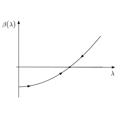
Figure 6.5: Schematic representation of the beta function (6.28).

and is seen to yield a nontrivial IR fixed point $\lambda^{*}\mbox{}^{2}=1/4\theta^{2}$ determined by the filling factor. More precisely, the strength of the repulsive coupling at the fixed point $\lambda^{*}=\pi(2l+1)$ increases with the number $2l+1$ of flux quanta bound to the electron. The presence of the fixed point shows that the CSGL theory undergoes a 2nd-order phase transition when the chemical potential of the composite particles tends to a critical value. As in the neutral case, it can be shown that the boson self-energy $\Sigma$ also vanishes at every loop order in the charged theory, and that the self-coupling parameter $\lambda$ is the only object that renormalizes. The 2nd-order phase transition described by the nontrivial IR fixed point has consequently again Gaussian exponents $\nu={\textstyle\frac{1}{2}},\;z=2$ [17]. It should be noted that only the location of the fixed point depends on $\theta$, the critical exponents—which in contrast to the strength of the coupling at the fixed point are independent of the regularization and renormalization scheme—are universal and independent of the filling factor. This “triviality” is in accord with the experimentally observed universality of the FQHE. A dependence of the critical exponents on $\theta$ could from the theoretical point of view hardly be made compatible with the hierarchy construction [84] which implies a cascade of phase transitions. From this viewpoint the present results are most satisfying: the CSGL theory is shown to encode a new type of field-induced 2nd-order quantum phase transition that is simple enough not to obscure the observed universality of the FQHE.

We stress again that in order to arrive at a realistic description of the FQHE, the CSGL theory has to be extended to include a $1/|{\bf x}|$-Coulomb potential and impurities. Both will change the critical behavior we found in this section. In particular, the Coulomb potential will change the Gaussian value $z=2$ into $z=1$.

6.4 Random Theory

In Sec. 6.2, we saw that in the absence of impurities repulsively interacting bosons undergo a 2nd-order quantum phase transition as function of the chemical potential. As was pointed out there, this universality class is of relevance to various condensed-matter systems. However, in most of the systems mentioned there, as well in ⁴He in porous media, impurities play an essential if not decisive role. For example, the two-dimensional superconductor-to-insulator transition investigated by Hebard and Paalanen [63] is driven by impurities. This means that, e.g., the correlation length $\xi$ diverges as $|\Delta_{\rm c}-\Delta|^{-\nu}$ when the disorder strength $\Delta$ characterizing the randomness approaches the critical value $\Delta_{\rm c}$. Hence, a realistic description of the critical behavior of these systems should include impurities.

To include these, we proceed as before and add the random term (3.78) to the nonrelativistic $|\phi|^{4}$-theory (3.1). The random field $\psi({\bf x})$ has the Gaussian distribution (3.79). We shall study the theory in the symmetrical state where the bare chemical potential is negative and the global U(1) symmetry unbroken. We therefore set $\mu_{0}=-r_{0}$ again, with $r_{0}>0$. We leave the number of space dimensions $d$ unspecified for the moment. As we remarked before, since $\psi({\bf x})$ depends only on the $d$ spatial dimensions, the impurities it describes should be considered as grains randomly distributed in space. When—as is required for the study of quantum critical phenomena—time is included, the static grains trace out straight worldlines. That is to say, these impurities are linelike in the quantum theory. It has been shown by Dorogovtsev [86] that the critical properties of systems with extended defects must be studied in a double $\epsilon$-expansion, otherwise no IR fixed point is found. The method differs from the usual $\epsilon$-expansion, in that it also includes an expansion in the defect dimensionality $\epsilon_{\rm d}$. To carry out this program in the present context, where the defect dimensionality is determined by the dimensionality of time, the theory has to be formulated in $\epsilon_{\rm d}$ time dimensions. The case of interest is $\epsilon_{\rm d}=1$, while in the opposite limit, $\epsilon_{\rm d}\rightarrow 0$, the random nonrelativistic $|\phi|^{4}$-theory reduces to the classical spin model with random (pointlike) impurities. Hence, $\epsilon_{\rm d}$ is a parameter with which quantum fluctuations can be suppressed. An expansion in $\epsilon_{\rm d}$ is a way to perturbatively include the effect of quantum fluctuations on the critical behavior. Ultimately, we will be interested in the case $\epsilon_{\rm d}=1$.

To calculate the quantum critical properties of the random theory, which have first been studied in [87], we will not employ the replica method [88], but instead follow Lubensky [89]. In this approach, the averaging over impurities is carried out for each Feynman diagram separately. The upshot is that only those diagrams are to be included which remain connected when $\Delta_{0}$, the parameter characterizing the Gaussian distribution of the impurities, is set to zero [90]. To obtain the relevant Feynman rules of the random theory we average the interaction term (3.78) over the distribution (3.79):

$$\int\mbox{D}\psi\,P(\psi)\exp\left[i^{\epsilon_{\rm d}}\int\mbox{d}^{\epsilon_{\rm d}}t\,\mbox{d}^{d}x\,\psi({\bf x})\,|\phi(x)|^{2}\right]=$$ (6.29)

$$\exp\left[{\textstyle\frac{1}{4}}i^{2\epsilon_{\rm d}}\Delta_{0}\int\mbox{d}^{\epsilon_{\rm d}}t\,\mbox{d}^{\epsilon_{\rm d}}t^{\prime}\,\mbox{d}^{d}x\,|\phi(t,{\bf x})|^{2}|\phi(t^{\prime},{\bf x})|^{2}\right].$$

The randomness is seen to result in a quartic interaction term which is nonlocal in time. The factor $i^{\epsilon_{\rm d}}$ appearing in (6.29) arises from the presence of $\epsilon_{\rm d}$ time dimensions, each of which is accompanied by a factor of $i$. The Feynman rules of the random theory are now easily obtained

$$= \frac{-i^{-\epsilon_{\rm d}}{\rm e}^{i(\omega_{1}+\omega_{2}+\cdots+\omega_{\epsilon_{\rm d}})\eta}}{\omega_{1}+\omega_{2}+\cdots+\omega_{\epsilon_{\rm d}}-{\bf k}^{2}-r_{0}+i\eta}$$

$$= -4i^{\epsilon_{\rm d}}\lambda_{0}$$

$$= i^{\epsilon_{\rm d}}(2\pi)^{\epsilon_{\rm d}}\delta^{\epsilon_{\rm d}}(\omega_{1}+\omega_{2}+\cdots+\omega_{\epsilon_{\rm d}})\Delta_{0},$$ (6.30)

where we note that the Lagrangian in $\epsilon_{\rm d}$ time dimensions involves instead of just one time derivative, a sum of $\epsilon_{\rm d}$ derivatives: $\partial_{t}\rightarrow\partial_{t_{1}}+\partial_{t_{2}}+\cdots+\partial_{t_{\epsilon_{\rm d}}}$.

Following Weichman and Kim [91], we evaluate the integrals over loop energies assuming that all energies are either positive or negative. This allows us to employ Schwinger’s propertime representation of propagators [92], which is based on the integral representation (3.47) of the gamma function. The energy integrals we encounter to the one-loop order can be carried out with the help of the equations

$$\int^{\prime}\frac{\mbox{d}^{\epsilon_{\rm d}}\omega}{(2\pi)^{\epsilon_{\rm d}}}\frac{1}{\omega_{1}+\omega_{2}+\cdots+\omega_{\epsilon_{\rm d}}-x\pm i\eta}=$$ (6.31)

$$-\frac{\Gamma(1-\epsilon_{\rm d})}{(2\pi)^{\epsilon_{\rm d}}}{\rm sgn}(x)|x|^{\epsilon_{\rm d}-1}\left({\rm e}^{\pm i\,{\rm sgn}(x)\pi\epsilon_{\rm d}}+1\right),$$

$$\int^{\prime}\frac{\mbox{d}^{\epsilon_{\rm d}}\omega}{(2\pi)^{\epsilon_{\rm d}}}\frac{{\rm e}^{i(\omega_{1}+\omega_{2}+\cdots+\omega_{\epsilon_{\rm d}})\eta}}{\omega_{1}+\omega_{2}+\cdots+\omega_{\epsilon_{\rm d}}-x+ix\eta}=$$ (6.32)

$$\frac{i\pi}{(2\pi)^{\epsilon_{\rm d}}\Gamma(\epsilon_{\rm d})}(i|x|)^{\epsilon_{\rm d}-1}\left[\sin({\textstyle\frac{1}{2}}\pi\epsilon_{\rm d})-\frac{{\rm sgn}(x)}{\sin({\textstyle\frac{1}{2}}\pi\epsilon_{\rm d})}\right].$$

The prime on the integrals is to remind the reader that the energy integrals are taken over only two domains with either all energies positive or negative. The energy integrals have been carried out by using again the integral representation (3.47) of the gamma function. In doing so, the integrals are regularized and—as is always the case with analytic regularizations—irrelevant divergences suppressed.

By differentiation with respect to $x$, Eq. (6.31) can, for example, be employed to calculate integrals involving integrands of the form $1/(\omega_{1}+\omega_{2}+\cdots+\omega_{\epsilon_{\rm d}}-x+i\eta)^{2}$. Is is easily checked that in the limit $\epsilon_{\rm d}\rightarrow 1$, where the energy integral can be performed with help of contour integration, Eqs. (6.31) and (6.32) reproduce the right results. When considering the limit of zero time dimensions ($\epsilon_{\rm d}\rightarrow 0$), it should be borne in mind that the energy integrals were taken over two separate domains with all energies either positive or negative. Each of these domains is contracted to a single point in the limit $\epsilon_{\rm d}\rightarrow 0$, so that one obtains a result which is twice that obtained by simply purging any reference to the time dimensions. The integral (6.32) contains an additional convergence factor $\exp(i\omega\eta)$ for each of the $\epsilon_{\rm d}$ energy integrals. This factor, which—as we remarked before—is typical for nonrelativistic quantum theories [51], is to be included in self-energy diagrams containing only one $\phi$-propagator.

Before studying the random theory, let us briefly return to the repulsively interacting bosons in the absence of impurities. In this case, there is no need for an $\epsilon_{\rm d}$-expansion and the formalism outlined above should yield results for arbitrary time dimensions $0\leq\epsilon_{\rm d}\leq 1$, interpolating between the classical and quantum limit. After the energy integrals have been performed with the help of Eqs. (6.31) and (6.32), the standard technique of integrating out a momentum shell can be applied to obtain the renormalization-group equations. For the correlation-length exponent $\nu$ we obtain in this way [30]

$$\nu=\frac{1}{2}\left[1+\frac{\epsilon}{2}\frac{m+1}{(m+4)-(m+3)\epsilon_{\rm d}}\cos^{2}({\textstyle\frac{1}{2}}\pi\epsilon_{\rm d})\right].$$ (6.33)

Here, $\epsilon=4-2\epsilon_{\rm d}-d$ is the deviation of the effective spacetime dimensionality from 4, where it should be noted that in (canonical) nonrelativistic theories, time dimensions have an engineering dimension twice that of space dimensions. (This property is brought out by the Gaussian value $z=2$ for the dynamic exponent $z$.) For comparison we have extended the theory (3.1) to include $m$ complex $\phi$-fields instead of just one field. In the classical limit, Eq. (6.33) gives the well-known one-loop result for a classical spin model with $2m$ real components [29],

$$\nu\rightarrow\frac{1}{2}\left(1+\frac{\epsilon}{2}\frac{m+1}{m+4}\right),$$ (6.34)

while in the quantum limit it gives the result $\nu\rightarrow\frac{1}{2}$, as required.

The exponent (6.33), and also the location of the fixed point, diverges when the number of time dimensions becomes $\epsilon_{\rm d}\rightarrow(m+4)/(m+3)$. Since this value is always larger than one, the singularity is outside the physical domain $0\leq\epsilon_{\rm d}\leq 1$. This simple example illustrates the viability of the formalism developed here to generate results interpolating between the classical and quantum limit.

We continue with the random theory. After the energy integrals have been carried out, it is again straightforward to derive the renormalization-group equations by integrating out a momentum shell $\Lambda/b<k<\Lambda$, where $\Lambda$ is a high-momentum cutoff and $b=\exp(l)$, with $l$ infinitesimal. Defining the dimensionless variables

$$\hat{\lambda}=\frac{K_{d}}{(2\pi)^{\epsilon_{\rm d}}}\lambda\Lambda^{-\epsilon};\;\;\;\hat{\Delta}=K_{d}\Delta\Lambda^{d-4};\;\;\;\hat{r}=r\Lambda^{-2},$$ (6.35)

where

$$K_{d}=\frac{2}{(4\pi)^{d/2}\Gamma({\textstyle\frac{d}{2}})}$$ (6.36)

is the area of a unit sphere in $d$ spatial dimensions divided by $(2\pi)^{d}$, we find [30]

$$\frac{\mbox{d}\hat{\lambda}}{\mbox{d}l} = \epsilon\hat{\lambda}-8\left[\Gamma(1-\epsilon_{\rm d})+(m+3)\Gamma(2-\epsilon_{\rm d})\right]\cos({\textstyle\frac{1}{2}}\pi\epsilon_{\rm d})\hat{\lambda}^{2}+6\hat{\Delta}\hat{\lambda}$$

$$\frac{\mbox{d}\hat{\Delta}}{\mbox{d}l} = (\epsilon+2\epsilon_{\rm d})\hat{\Delta}+4\hat{\Delta}^{2}-16(m+1)\Gamma(2-\epsilon_{\rm d})\cos({\textstyle\frac{1}{2}}\pi\epsilon_{\rm d})\hat{\lambda}\hat{\Delta}$$

$$\frac{\mbox{d}\hat{r}}{\mbox{d}l} = 2\hat{r}+4\pi\frac{m+1}{\Gamma(\epsilon_{\rm d})}\frac{\cos^{2}({\textstyle\frac{1}{2}}\pi\epsilon_{\rm d})}{\sin({\textstyle\frac{1}{2}}\pi\epsilon_{\rm d})}\hat{\lambda}-\hat{\Delta}.$$ (6.37)

These results are to be trusted only for small values of $\epsilon_{\rm d}$. For illustrative purposes we have, however, kept the full $\epsilon_{\rm d}$ dependence. The set of equations yields the fixed point

$$\hat{\lambda}^{*} = \frac{1}{16\cos({\textstyle\frac{1}{2}}\pi\epsilon_{\rm d})\Gamma(1-\epsilon_{\rm d})}\,\frac{\epsilon+6\epsilon_{\rm d}}{2m(1-\epsilon_{\rm d})-1}$$ (6.38)

$$\hat{\Delta}^{*} = \frac{1}{4}\frac{m(1-\epsilon_{\rm d})(2\epsilon_{\rm d}-\epsilon)+2\epsilon_{\rm d}(4-3\epsilon_{\rm d})+\epsilon(2-\epsilon_{\rm d})}{2m(1-\epsilon_{\rm d})-1},$$

and the critical exponent

$$\nu=\frac{1}{2}+\frac{\epsilon+2\epsilon_{\rm d}}{16}+\frac{m+1}{16}\frac{(6\epsilon_{\rm d}+\epsilon)[\epsilon_{\rm d}+\cos(\pi\epsilon_{\rm d})]}{2m(1-\epsilon_{\rm d})-1}.$$ (6.39)

The dynamic exponent is given by $z=2+\hat{\Delta}^{*}$. When the equations are expanded to first order in $\epsilon_{\rm d}$, we recover the IR fixed point found by Weichman and Kim [91] using an high-energy cutoff:

$$\hat{\lambda}^{*}=\frac{1}{16}\frac{\epsilon+6\epsilon_{\rm d}}{2m-1};\;\;\;\hat{\Delta}^{*}=\frac{1}{4}\frac{(2-m)\epsilon+2(m+4)\epsilon_{\rm d}}{2m-1},$$ (6.40)

with the critical exponent

$$\nu=\frac{1}{2}\left[1+\frac{1}{8}\frac{3m\epsilon+(5m+2)2\epsilon_{\rm d}}{2m-1}\right].$$ (6.41)

The value of the critical exponent (6.41) should be compared with that of the classical spin model with $2m$ components in the presence of random impurities of dimension $\epsilon_{\rm d}$ [86]:

$$\nu=\frac{1}{2}\left[1+\frac{1}{8}\frac{3m\epsilon+(5m+2)\epsilon_{\rm d}}{2m-1}\right].$$ (6.42)

Taking into account that in a nonrelativistic quantum theory, time dimensions count double as compared to space dimensions, we see that both results are equivalent. As to the dynamic exponent, notice that the perturbative result $z=2+\hat{\Delta}^{*}$, with $\hat{\Delta}^{*}$ given by (6.40), is far away from the exact value $z=d$ for $\epsilon_{\rm d}=1$ [80].

6.5 Experiments

6.5.1 Superconductor-To-Insulator Transition

The first experiments we wish to discuss are those performed by Hebard and Paalanen on superconducting films in the presence of random impurities [63, 85]. It has been predicted by Fisher [93] that with increasing applied magnetic field such systems undergo a zero-temperature transition into an insulating state. (For a critical review of the experimental data available in 1993, see Ref. [2].)

Let us restrict ourselves for the moment to the $T\Delta$-plane of the phase diagram by setting the applied magnetic field $H$ to zero. For given disorder strength $\Delta$, the system then undergoes a Kosterlitz-Thouless transition induced by the unbinding of magnetic vortex pairs at a temperature $T_{\rm KT}$ well below the bulk transition temperature (see Sec. 4.3). The Kosterlitz-Thouless temperature is gradually suppressed to zero when the disorder strength approaches criticality $\Delta\rightarrow\Delta_{\rm c}$. The transition temperature scales with the correlation length $\xi\sim|\Delta_{\rm c}-\Delta|^{-\nu}$ as $T_{\rm KT}\sim\xi^{-z}$.

In the $H\Delta$-plane, i.e., at $T=0$, the situation is as follows. For given disorder strength, there is now at some critical value $H_{\rm c}$ of the applied magnetic field a phase transition from a superconducting state of pinned vortices and condensed Cooper pairs to an insulating state of pinned Cooper pairs and condensed vortices. The condensation of vortices disorder the ordered state as happens in classical, finite temperature superfluid- and superconductor-to-normal phase transitions [34]. When the disorder strength approaches criticality again, $H_{\rm c}$ is gradually suppressed to zero. The critical field scales with $\xi$ as $H_{\rm c}\sim\Phi_{0}/\xi^{2}$. In fact, this expresses a more fundamental result, namely that the scaling dimension $d_{\bf A}$ of ${\bf A}$ is one,

$$d_{\bf A}=1,$$ (6.43)

so that $|{\bf A}|\sim\xi^{-1}$. From this it in turn follows that $E\sim\xi_{t}^{-1}\xi^{-1}\sim\xi^{-(z+1)}$, and that the scaling dimension $d_{A_{0}}$ of $A_{0}$ is $z$,

$$d_{A_{0}}=z,$$ (6.44)

so that $A_{0}\sim\xi_{t}^{-1}\sim\xi^{-z}$. Together, the scaling results for $T_{\rm KT}$ and $H_{\rm c}$ imply that [93]

$$H_{\rm c}\sim T_{\rm KT}^{2/z}.$$ (6.45)

This relation, linking the critical field of the zero-temperature transition to the Kosterlitz-Thouless temperature, provides a direct way to measure the dynamic exponent $z$ at the $H=0$, $T=0$ transition. This has been first done by Hebard and Paalanen [63, 85]. Their experimental determination of $T_{\rm KT}$ and $H_{\rm c}$ for five different films with varying amounts of impurities confirmed the relation (6.45) with $2/z=2.04\pm 0.09$. The zero-temperature critical fields were obtained by plotting $\mbox{d}\rho_{xx}/\mbox{d}T|_{H}$ versus $H$ at the lowest accessible temperature and interpolating to the the field where the slope is zero. The resulting value $z=0.98\pm.04$ is in accordance with Fisher’s prediction [93], $z=1$, for a random system with a $1/|{\bf x}|$-Coulomb potential.

Hebard and Paalanen [63] also investigated the field-induced zero-temperature transition. The control parameter is here $\delta\propto H-H_{\rm c}$. When plotted as function of $|H-H_{\rm c}|/T^{1/\nu_{H}z_{H}}$ they saw their resistivity data collapsing onto two branches; an upper branch tending to infinity for the insulating state, and a lower branch bending down for the superconducting state. The unknown product $\nu_{H}z_{H}$ is experimentally determined by looking for which value the best scaling behavior is obtained. Further experiments carried out by Yazdani and Kapitulnik [94] also determined the product $\nu_{H}(z_{H}+1)$ (see below). The two independent measurements together fix the critical exponents $\nu_{H}$ and $z_{H}$ separately. From their best data, Yazdani and Kapitulnik extracted the values [94]

$$z_{H}=1.0\pm 0.1,\;\;\;\;\nu_{H}=1.36\pm 0.05.$$ (6.46)

6.5.2 Quantum-Hall Systems

We continue to discuss the field-induced quantum phase transitions in quantum Hall systems. Since an excellent discussion recently appeared in the literature [4], we shall be brief, referring the reader to that review for a more thorough discussion and additional references.

One can image transitions from one Hall liquid to another Hall liquid with a different (integer or fractional) filling factor, or to the insulating state. Experiments seem to suggest that all the quantum-Hall transitions are in the same universality class. The transitions are probed by measuring the resistivities $\rho_{xx}$ and $\rho_{xy}$. From the dependence of the conductivity $\sigma$ on the superfluid mass density, Eq. (6.19), and the scaling relation (6.14), it follows that it scales as [95]

$$\sigma\sim\xi^{-(d-2)}.$$ (6.47)

In other words, the scaling dimension of the conductivity and therefore that of the resistivity is zero in two space dimensions. On account of the general finite-size scaling form (6.3), we then have in the limit $|{\bf k}|\rightarrow 0$:

$$\rho_{xx/y}(k_{0},H,T)=\varrho_{xx/y}(k_{0}/T,|\delta|^{\nu z}/T),$$ (6.48)

where the distance to the zero-temperature critical point is measured by $\delta\propto H-H_{\nu_{H}}^{\pm}\sim T^{1/\nu z}$. This scaling of the width of the transition regime with temperature has been corroborated by DC or $k_{0}=0$ experiments on various transitions between integer quantum-Hall states which were all found to yield the value $1/\nu z=0.42\pm 0.04$ [96].

A second measurement of the critical exponents involves the applied electric field. As we have seen above, it scales as $E\sim\xi^{-(z+1)}$, so that for the DC resistivities we now obtain the scaling form:

$$\rho_{xx/y}(H,T,E)=\varrho_{xx/y}(|\delta|^{\nu z}/T,|\delta|^{\nu(z+1)}/E).$$ (6.49)

The scaling $|\delta|\sim E^{1/\nu(z+1)}$ has again been corroborated by experiment which yielded the value $\nu(z+1)\approx 4.6$ [97]. Together with the previous result obtained from the temperature scaling this gives

$$z\approx 1,\;\;\;\;\nu\approx 2.3.$$ (6.50)

The value of the dynamic exponent strongly suggests that it is a result of the presence of the $1/|{\bf x}|$-Coulomb potential. The correlation length exponent $\nu$ is large.

6.5.3 $2d$ Electron Systems

Recently, silicon MOSFET’s at extremely low electron number densities has been studied [98, 99, 100, 101]. Earlier experiments at higher densities seemed to confirm the general believe, based on the work by Abrahams et al. [95], that such two-dimensional electron systems do not undergo a quantum phase transition. In that influential paper, it was demonstrated that even weak disorder is sufficient to localize the electrons at the absolute zero of temperature thus excluding conducting behavior. Electron-electron interactions were however not included. As we saw in Sec. 3.2, at low densities, the $1/|{\bf x}|$-Coulomb interaction becomes important and the analysis of Abrahams et al. [95] no longer applies.

The recent experiments have revealed a zero-temperature conductor-to-insulator transition triggered by a change in the charge carrier density $\bar{n}$. That is, the distance to the critical point is in these systems measured by $\delta\propto\bar{n}-\bar{n}_{\rm c}$. Like in the quantum-Hall systems, these transitions are probed by measuring the resistivity. It scales with temperature near the transition according to the scaling form (6.49) with $H$ set to zero. For $\bar{n}<\bar{n}_{\rm c}$, where the Coulomb interaction is dominant and fluctuations in the charge carrier density are suppressed, the electron system is insulating. On increasing the density, these fluctuations intensify and at the critical value $\bar{n}_{\rm c}$, the system reverts to a conducting phase. By plotting their conductivity data as function of $T/|\delta|^{\nu z}$ with $\nu z=1.6\pm 0.1$, Popovíc, Fowler, and Washburn [101] saw it collapse onto two branches; the upper branch for the conducting side of the transition, and the lower one for the insulating side. A similar collapse with a slightly different value $1/\nu z=0.83\pm 0.08$ was found in Ref. [99], where also the collapse of the data when plotted as function of $|\delta|/E^{1/\nu(z+1)}$ was obtained. The best collapse resulted for $1/(z+1)\nu=0.37\pm 0.01$, leading to

$$z=0.8\pm 0.1,\;\;\;\;\nu=1.5\pm 0.1.$$ (6.51)

The value for the dynamic exponent is close to the expected value $z=1$ for a charged system with a $1/|{\bf x}|$-Coulomb interaction, while that of $\nu$ is surprisingly close to the value (6.46) found for the superconductor-to-insulator transition.

A further experimental result for these two-dimensional electron systems worth mentioning is the suppression of the conducting phase by an applied magnetic field found by Simonian, Kravchenko, and Sarachik [100]. They applied the field parallel to the plane of the electrons instead of perpendicular as is done in quantum-Hall measurements. In this way, the field presumably couples only to the spin of the electrons and the complications arising from orbital effects do not arise. At a fixed temperature, a rapid initial raise in the resistivity was found with increasing field. Above a value of about 20 kOe, the resistivity saturates. It was pointed out that both the behavior in a magnetic filed, as well as in zero field strongly resembles that near the superconductor-to-insulator transition discussed above, suggesting that the conducting phase might in fact be superconducting.

6.5.4 Conclusions

We have seen that general scaling arguments can be employed to understand the scaling behavior observed in various quantum phase transitions. Most of the experiments seem to confirm the expected value $z=1$ for a random system with a $1/|{\bf x}|$-Coulomb interaction. The number of different universality classes present is yet not known. Even if the conductor-to-insulator transition observed in silicon MOSFET’s at low electron number densities turns out to be in the same universality class as the superconductor-to-insulator transition, there are still the field-induced transitions in quantum-Hall systems, which have a larger correlation-length exponent.

The paradigm provided by a repulsively interacting Bose gas, seems to be a good starting point to describe the various systems. However, high-precision estimates calculated from this theory with impurities and a $1/|{\bf x}|$-Coulomb interaction included are presently lacking.

Bibliography

- [1] D. I. Uzunov, Introduction to the Theory of Critical Phenomena (World Scientific, Singapore, 1993).
- [2] T. Liu and A. M. Goldman, Mod. Phys. Lett. B 8, 277 (1994).
- [3] S. Sachdev, in Proceedings of teh 19th IUPAP International Conference on Statistical Physics, Xiamen, China, 1995, edited by B. -L. Hao (World Scientific, Singapore, 1995), p. 289 [e-print cond-mat/9508080 (1995)].
- [4] S. L. Sondhi, S. M. Girvin, J. P. Carini, and D. Shahar, Rev. Mod. Phys. 69, 315 (1997).
- [5] C. M. Fraser, Z. Phys. C 28, 101 (1985); I. J. R. Aitchison and C. M. Fraser, Phys. Rev. D 31, 2605 (1985).
- [6] E. P. Gross, Nuovo Cimento 20, 454 (1961); L. P. Pitaevskii, Sov. Phys. JETP 13, 451 (1961).
- [7] N. N. Bogoliubov, J. Phys. USSR 11, 23 (1947).
- [8] S. T. Beliaev, Sov. Phys. JETP 7, 289 (1958).
- [9] N. M. Hugenholtz and D. Pines, Phys. Rev. 116, 489 (1959).
- [10] J. Bernstein and S. Dodelson, Phys. Rev. Lett. 66, 683 (1991); K. M. Benson, J. Bernstein, and S. Dodelson, Phys. Rev. D 44, 2480 (1991).
- [11] J. Gavoret and P. Nozières, Ann. Phys. (N.Y.), 28, 349 (1964).
- [12] A. M. J. Schakel, Int. J. Mod. Phys. B 8, 2021 (1994).
- [13] A. M. J. Schakel, Mod. Phys. Lett. B 4, 927 (1990).
- [14] A. M. J. Schakel, Int J. Mod. Phys. B 10, 999 (1996).
- [15] P. W. Anderson, Rev. Mod. Phys. 38 298 (1966).
- [16] H. Leutwyler, Phys. Rev. D 49, 3033 (1994).
- [17] A. M. J. Schakel, Nucl. Phys. B [FS] 453, 705 (1995).
- [18] M. Greiter, F. Wilczek, and E. Witten, Mod. Phys. Lett. B 3, 903 (1989).
- [19] J. F. Donoghue, Phys. Rev. D 50, 3847 (1994); e-print gr-qc/9512024 (1995).
- [20] T. Y. Cao and S. S. Schweber, Synthese 97 (1993); in Renormalization, edited by L. M. Brown (Springer-Verlag, Berlin, 1993).
- [21] P. B. Weichman, Phys. Rev. B 38, 8739 (1988).
- [22] A. L. Fetter and J. D. Walecka, Quantum Theory of Many-Particle Systems (McGraw-Hill, New York, 1971).
- [23] E. H. Lieb and W. Liniger, Phys. Rev. 130, 1605 (1963); E. H. Lieb, Phys. Rev. 130, 1616 (1963).
- [24] D. I. Uzunov, Phys. Lett. A 87, 11 (1981).
- [25] U. C. Täuber and D. R. Nelson, Phys. Rep. 289, 157 (1997).
- [26] O. Penrose and L. Onsager, Phys. Rev. 104, 576 (1956).
- [27] P. Nozières and D. Pines, The Theory of Quantum Liquids (Addison-Wesley, New York, 1990), Vol. II.
- [28] L. S. Brown, Quantum Field Theory (Cambridge University Press, Cambridge, 1992).
- [29] S. K. Ma, Modern Theory of Critical Phenomena (Benjamin, London, 1976).
- [30] A. M. J. Schakel, Phys. Lett. A, 224, 287 (1997).
- [31] S. Giorgini, L. Pitaevskii, and S. Stringari, Phys. Rev. B 49, 12938 (1994).
- [32] K. Huang and H.-F. Meng, Phys. Rev. Lett. 69, 644 (1992).
- [33] A. L. Fetter, Phys. Rev. 138, 429 (1965).
- [34] H. Kleinert, Gauge Fields in Condensed Matter (World Scientific, Singapore, 1989), Vol. I.
- [35] H. Kleinert, Int. J. Mod. Phys. A 7, 4693 (1992).
- [36] H. Kleinert, in Formation and Interactions of Topological Defects, Proceedings NATO ASI, Cambridge, 1994, edited by A. C. Davis and R. Brandenburger (Plenum, New York, 1995).
- [37] H. Lamb, Hydrodynamics (Dover, New York, 1945), p. 230.
- [38] W. Yourgrau and S. Mandelstam, Variational Principles in Dynamics and Quantum Theory (Pitman, London, 1968).
- [39] M. V. Berry, Proc. Roy. Soc. A 392, 45 (1984).
- [40] F. D. M. Haldane and Y. -S. Wu, Phys. Rev. Lett. 55, 2887 (1985).
- [41] F. Lund, Physica A 159, 245 (1991).
- [42] E. J. Yarmchuk and R. E. Packard, J. Low Temp. Phys. 46, 479 (1982).
- [43] V. L. Berezinskii, Sov. Phys. JETP 34, 610 (1972).
- [44] J. M. Kosterlitz and D. J. Thouless, J. Phys. C 6, 1181 (1973).
- [45] D. R. Nelson and J. M. Kosterlitz, Phys. Rev. Lett. 39, 1201 (1977).
- [46] S. Schenker, in Recent Advances in Field Theory and Statistical Mechanics, proceedings of Les Houches summerschool, Session XXXIX, 1982, edited by J. B. Zuber and R. Stora (Elsevier, Amsterdam, 1984).
- [47] J. Bardeen, L. N. Cooper, J. R. Schrieffer, Phys. Rev. 108, 1175 (1957).
- [48] S. Weinberg, Prog. Theor. Phys. Suppl. 86, 43 (1986).
- [49] H. Kleinert, Fortschr. Phys. 26, 565 (1978).
- [50] A. J. Leggett in Modern Trends in the Theory of Condensed Matter, edited by A. Pekalski and J. Przystawa (Springer-Verlag, Berlin, 1980), p. 13.
- [51] R. D. Mattuck, A Guide to Feynman Diagrams in the Many-Body Problem (McGraw-Hill, New York, 1976).
- [52] R. Haussmann, Z. Phys. B 91, 291 (1993).
- [53] M. Drechsler and W. Zwerger, Ann. Phys. (Germany) 1, 15 (1992).
- [54] C. A. R. Sá de Melo, M. Randeria, and J. R. Engelbrecht, Phys. Rev. Lett. 71, 3202 (1993).
- [55] M. Marini, F. Pistolesi, and G. C. Strinati, e-print cond-mat/9703160 (1997).
- [56] U. Eckern, G. Schön, and V. Ambegaokar, Phys. Rev. 30, 6419 (1989).
- [57] M. Randeria, J. -M. Duan, and L. -Y. Shieh, Phys. Rev. B 41, 327 (1990).
- [58] F. A. Schaposnik, Phys. Rev. D 18, 1183 (1978).
- [59] J. Pearl, in Low Temperature Physics—LT9, edited by J. G. Danut, D. O. Edwards, F. J. Milford, and M. Yagub (Plenum, New York, 1965).
- [60] P. G. de Gennes, Superconductivity of Metals and Alloys (Addison-Wesley, New York, 1966).
- [61] M. R. Beasley, J. E. Mooij, and T. P. Orlando, Phys. Rev. Lett. 42, 1165 (1979).
- [62] M.-C. Cha, M. P. A. Fisher, S. M. Girvin, M. Wallin, and A. P. Young, Phys. Rev. B 44, 6883 (1991); S. M. Girvin, M. Wallin, M.-C. Cha, M. P. A. Fisher, and A. P. Young, Prog. Theor. Phys. Suppl. 107, 135 (1992).
- [63] A. F. Hebard and M. A. Paalanen, Phys. Rev. Lett. 65, 927 (1990).
- [64] R. B. Laughlin, Phys. Rev. Lett. 50, 1395 (1983).
- [65] V. L. Ginzburg and L. D. Landau, Zh. Eksp. Teor. Fiz. 20, 1064 (1950); reprinted in L. D. Landau, Collected Papers (Pergamon, London, 1965), p. 546.
- [66] L. P. Gorkov, Sov. Phys. JETP 9, 1364 (1959).
- [67] S. M. Girvin, in The Quantum Hall Effect, edited by R. E. Prange and S. M. Girvin (Springer-Verlag, Berlin, 1986), Ch. 10; S. M. Girvin and A. H. MacDonald, Phys. Rev. Lett. 58, 1252 (1987).
- [68] S.-C. Zhang, T. H. Hansson, and S. Kivelson, Phys. Rev. Lett. 62, 82 (1989).
- [69] S.-C. Zhang, Int. J. Mod. Phys. B 6, 25 (1992).
- [70] F. Wilczek, Fractional Statistics and Anyon Superconductivity (World Scientific, Singapore, 1990).
- [71] D. P. Arovas, J. R. Schrieffer, and F. Wilczek, Phys. Rev. Lett. 53, 722 (1984).
- [72] B. Widom, J. Chem. Phys. 43, 3892 (1965); 43, 3898 (1965).
- [73] M. P. A. Fisher, P. B. Weichman, G. Grinstein, and D. S. Fisher, Phys. Rev. B 40, 546 (1989).
- [74] J. A. Hertz, Phys. Rev. B 14, 1165 (1976).
- [75] I. Affleck, Phys. Rev. B 41, 6697 (1990).
- [76] T. R. Kirkpatrick and D. Belitz, Phys. Rev. Lett. 76, 2571 (1996).
- [77] M. P. A. Fisher, G. Grinstein, and S. M. Girvin, Phys. Rev. Lett. 64, 587 (1990).
- [78] O. Bergman, Phys. Rev. D 46, 5474 (1992).
- [79] G. G. Batrouni, R. T. Scalettar, and G. T. Zimanyi, Phys. Rev. Lett. 65, 1765 (1990).
- [80] D. S. Fisher and M. P. A. Fisher, Phys. Lett. 61, 1847 (1988).
- [81] S. Coleman and B. Hill, Phys. Lett. B 159, 184 (1985).
- [82] J. D. Lykken, J. Sonneschein, and N. Weiss, Int. J. Mod. Phys. A 6, 1335 (1991).
- [83] G. Lozano, Phys. Lett. B 283, 70 (1992); O. Bergman and G. Lozano, Ann. Phys. (N.Y.) 229, 416 (1994).
- [84] F. D. M. Haldane, Phys. Rev. Lett. 51, 605 (1983); B. I. Halperin, Phys. Rev. Lett. 52, 1583 (1984).
- [85] A. F. Hebard and M. A. Paalanen, Helv. Phys. Act. 65, 197 (1992).
- [86] S. N. Dorogovtsev, Phys. Lett. A 76, 169 (1980).
- [87] E. R. Korutcheva and D. I. Uzunov, Phys. Lett. A 106, 175 (1984).
- [88] G. Grinstein and A. Luther, Phys. Rev. B 13, 1329 (1976).
- [89] T. C. Lubensky, Phys. Rev. B 11, 3573 (1975).
- [90] For a review see, for example, J. A. Hertz, Physica Scripta T10, 1 (1985).
- [91] P. B. Weichman and K. Kim, Phys. Rev. B 40, 813 (1989).
- [92] J. Schwinger, Phys. Rev. 82, 664 (1951).
- [93] M. P. A. Fisher, Phys. Rev. Lett. 65, 923 (1990).
- [94] A. Yazdani and A. Kapitulnik, Phys. Rev. Lett. 74, 3037 (1995).
- [95] E. Abrahams, P. W. Anderson, D. C. Licciardello, and T. V. Ramakrishnan, Phys. Rev. Lett. 42, 637 (1979).
- [96] H. P. Wei, D. C. Tsui, M. A. Paalanen, and A. M. M. Pruisken, Phys. Rev. Lett. 61, 1294 (1988).
- [97] H. P. Wei, L. W. Engel, and D. C. Tsui, Phys. Rev. B 50, 14609 (1994).
- [98] S. V. Kravchenko, G. V. Kravchenko, J. E. Furneaux, V. M. Pudalov, and M. D’Iorio, Phys. Rev. B 50, 8039 (1994); S. V. Kravchenko, W. E. Mason, G. E. Bowker, J. E. Furneaux, V. M. Pudalov, and M. D’Iorio, Phys, Rev. 51, 7038 (1995).
- [99] S. V. Kravchenko, D. Simonian, M. P. Sarachik, W. E. Mason, and J. E. Furneaux, Phys. Rev. Lett. 77, 4938 (1996).
- [100] D. Simonian, S. V. Kravchenko, and M. P. Sarachik, e-print cond-mat/9704071 (1997).
- [101] D. Popovíc, A. B. Fowler, and S. Washburn, e-print cond-mat/9704249 (1997).