Renormalization group analysis of the quantum non-linear sigma model with a damping term

Abstract

We investigate the behavior of the zero-temperature quantum non-linear sigma model in $d$ dimensions in the presence of a damping term of the form $f(\omega)\sim|\omega|^{\alpha}$, with $1\leq\alpha<2$. We find two fixed points: a spin-wave fixed point FP1 showing a dynamic scaling exponent $z=1$ and a dissipative fixed point FP2 with $z>1.$ In the framework of the $\epsilon$-expansion it is seen that there is a range of values $\alpha_{*}(d)\leq\alpha\leq 2$ where the point FP1 is stable with respect to FP2, so that the system realizes a $z=1$ quantum critical behavior even in the presence of a dissipative term. However, reasonable arguments suggest that in $d=2$ this range is very narrow. In the broken symmetry phase we discuss a phenomenological scaling approach, treating damping as a perturbation of the ordered ground state. The relation of these results with the pseudogap effect observed in underdoped layered cuprates is discussed.

, and

1 Introduction

The presence of an antiferromagnetic (AF) phase rapidly replaced by an anomalous metallic phase upon doping is one of the prominent features of the phase diagram of high temperature superconducting cuprates [1, 2]. Indeed it was early suggested [3] that the proximity to an insulating magnetic phase together with the nearly twodimensional structure of these materials could be responsible for the superconducting and anomalous normal-state (i.e. non-Fermi liquid) properties of these systems via the creation of a quantum-disordered spin liquid (resonating-valence-bond state). Since then a great deal of attention has been devoted to the fascinating interplay between magnetism and charge degrees of freedom, leading to various theoretical proposals and to different scenarios for the metal-insulator transition at low doping.

One scenario is based on the tendency of a magnetically ordered phase to segregate the additional holes due to doping [4]. The tendency to phase separation is then frustrated by the Coulombic repusion between the segregated carriers [5], thus leading to formation of hole-rich domain walls separating AF domains in the form of stripe textures. Within this scenario, pseudogaps naturally arise in the underdoped phase of the materials as a consequence of stripe fluctuations and local pair formation [6]. Obviously this will substantially affect the transition to the AF insulating phase at low doping [7, 8].

The transition between a magnetically ordered phase and a metallic state can also be strongly affected by extrinsic ingredients like the disorder induced by dopant ions (Sr or Zn in the case of ${\rm La_{2-x-y}Sr_{x}Zn_{y}CuO_{4}}$). This may lead to the formation of local random magnetic moments giving rise to spin-glass ordering between the AF insulating and the paramagnetic metallic (PM) phases [9, 10, 11, 12, 1].

The stripe and the spin-glass scenarios clearly illustrate the complicated and rich nature that the AF-PM transition may take. However, other proposals are more directly related to magnetism and to the contiguity between the AF and the metallic phase. These proposals start from the seminal work of Ref. [13] showing that the materials with half-filled CuO₂ planes are suitably described in terms of a twodimensional quantum Heisenberg AF model with very small interplanar coupling. Following work [14, 15, 16, 17, 18] suggested that, although the 2D model displays long-range order at $T=0$, upon doping the added charges enhance the quantum spin fluctuations thus driving the system into a disordered state even at zero temperature (quantum disordered phase) [14]. The occurrence of an AF quantum critical point (QCP) provides a natural framework to intepret the scaling behavior at low temperatures and low frequencies of the of the $q$-integrated magnetic susceptibility $\chi(\omega)=\int\,\mathrm{d}^{2}q\,\chi(\boldsymbol{q},\omega)$. The susceptibility $\chi(\omega)$ can be experimentally determined via magnetic resonance measurements of the nuclear copper spin-echo decay rate, $T_{2G}^{-1}$ and spin-lattice relaxation rate, $T_{1}^{-1}$ [19, 2]. It is seen that in a range of temperatures $T_{*}<T<T_{\mathrm{cr}}$, depending on doping, $T_{1}T/T_{2G}=\mathrm{const}$ [20]. Assuming the scaling relations [14], $\chi(\boldsymbol{q},\omega)\sim\xi^{2-\eta}\hat{\chi}(|\boldsymbol{q}-\boldsymbol{Q}_{\mathrm{AF}}|\xi,\omega/T)$ and $\xi\sim T^{-1/z}$, with $z$ a dynamic critical exponent, $\eta$ an anomalous dimension, $\boldsymbol{Q}_{\mathrm{AF}}$ the antiferromagnetic ordering wave-vector, $\xi$ the correlation length, $\hat{\chi}$ a scaling function, one gets $T_{1}T/T_{2G}\sim T^{1-1/z}$ [17, 18]. The constancy of this ratio is thus interpreted as the signature of a critical behavior corresponding to a $z=1$ value of the dynamic index [17, 18, 21, 22, 23]. The strong critical spin fluctuations occurring at the AF-QCP have also been claimed to provide a possible source of pairing and normal-state anomalies.

Despite the apparent simplicity of a scenario involving a direct transition between an insulating AF phase and a PM phase, such a transition is far from being trivial and is still an open problem. The main difficulty is in the lack of a microscopic model being able to smoothly interpolate between an insulating AF ordered phase with gapped charge excitation and a PM phase. On the one hand, the insulating AF phase is suitably represented by the Heisenberg model and, in particular, the long-wavelength and low frequency behavior of spin fluctuations in the CuO₂ planes can be well described by the quantum non-linear sigma model [13], which at zero temperature and in two spatial dimensions is characterized by the action

$$S=\frac{1}{2g}\int\,\mathrm{d}\omega\,\mathrm{d}^{2}k\left(k^{2}+\frac{\omega^{2}}{c^{2}}\right)\boldsymbol{\phi}_{\boldsymbol{k},\omega}\cdot\boldsymbol{\phi}_{-\boldsymbol{k},-\omega}$$ (1)

Here $\boldsymbol{\phi}$ is a three-component vector field subject to the real-space constraint $\phi_{\boldsymbol{x},\tau}^{2}=1$ which describes the local staggered magnetization, and $g$ is a coupling constant.

It was first argued in [14] that this description could be carried over to the case of the lightly doped compounds. In fact, one can think that in this case the $\boldsymbol{\phi}$ field continues giving an effective description of the electron spins localized on the Cu sites of the lattice, while the presence of itinerating holes provides a finite renormalization of the coupling constant. The theory described by the action (1), besides having the correct symmetries, realizes a zero-temperature transition for a given critical value $g_{\mathrm{c}}$ of the coupling (see [13, 24] for the quantum version and [25, 26, 27] for the classical theory) thus providing a good model for the physical picture of the AF-QCP [15]. From this point of view the $z=1$ value of the dynamic scaling exponent is a simple consequence of the Lorentz invariance of (1).

However, it is clear that the non-linear $\sigma$ model does not properly describe the low-energy charge excitations, which are characteristic of a metallic state possibly providing a damping mechanism for spin-waves (see, e.g., case B of Ref. [28]). Therefore the model in Eq. 1 provides a good description of a transition between an insulating (charge-gapped) AF (AFI) and an insulating paramagnet (PI)., but it appears to be inappropriate when spin-waves can decay in low-energy particle-hole excitations.

On the other hand, attempts have also been made to provide a microscopic basis for the transition to a PM phase. In this regard two distint cases A and B depending on the shape of the Fermi surface in the metal were investigated in Ref. [28] within a spin-density-wave approach. In case A the AF wavevector ${\boldsymbol{Q}}_{\mathrm{AF}}=(\pi/a,\pi/a)$ ($a$ is the lattice spacing) was not able to connect points of the Fermi surface, so that momentum and energy conservation did not allow the decay of spin-waves in particle-hole pairs. In this case the transition was naturally characterized by a dynamic critical index $z=1$. In case B, instead, there were (“hot”) points on the Fermi surface connected by ${\boldsymbol{Q}}_{\mathrm{AF}}$ so that low-energy particle-hole pairs could be created by the decay of low-energy spin-waves. However, in both cases, A and B, the phase with AF long-range order is metallic and therefore the model does not suitably describe a transition between an AFI and a PM . The case A above shares some common features with a mixed spin-fermion model without a three-body (i.e. Kondo-like) direct coupling between the local moments and the fermion spins [29]. This model has been shown [30] to display a $T=0$ transition between a metallic (Fermi liquid) phase with spin commensurate long-range order and a metallic (also Fermi liquid) quantum disordered phase. Owing to the absence of the three body coupling responsible for the direct spin-wave decay into particle-hole pairs, also the QCP of this model is characterized by $z=1$.

To the best of our knowledge no simple microscopic modelization is presently available to describe a direct AFI-PM transition. Of course the possibilities remain open that other extrinsic mechanisms (stripes, disorder, …) provide intermediate steps between the AFI and the PM phases. Alternatively, one may also envisage that an AFI to a PI phase transition occurs first at lower doping, followed at slightly larger doping by a PI-PM transition between two spin-disordered phases.

Together with the basic difficulty outlined above, the additional question arises concerning the observed $z=1$ critical behavior in the underdoped phase of the cuprates and the way this can be reconciled with the metallic character of this phase. In particular it is believed that the Fermi surface of the cuprates in the metallic phase contains “hot” points connected by the AF wavevector. Therefore it should be possible for the spin-waves of arbitrarily low energy to decay into particle-hole pairs and get overdamped. This would lead to a relaxational behavior contrasting with the $z=1$ (i.e. propagating) critical behavior of the spin-waves. Moreover, by accepting a $z=2$ critical behavior in the metallic phase, it remains to clarify how this may turn into the natural propagating behavior, which characterizes the spin excitations in the ordered side of the QCP. This latter difficulty was also encountered and stressed by the authors of Ref. [28] for their case B: within their mean-field description a $z=2$ behavior was obtained both in the disordered and the ordered AF (metallic) phases. This suggested that the simple formulation B of the mean-field SDW model was only applicable on the disordered side of (and not too close to) the AF-QCP.

In the present paper we will not attempt to find a microscopic foundation to a direct AFI-PM transition, but we will instead start from a semiphenomenological point of view by introducing a field-theoretical generalization of the non-linear $\sigma$ model action (1) to investigate a) the condition to be fullfilled by a simple ($\boldsymbol{k}$-independent) damping term in order to maintain a $z=1$ critical behavior; b) how in the $z>1$ case an additional crossover energy must behave in the ordered phase to provide a scale separating damped spin excitations at high energy and propagating spin excitations at low energy.

The resulting theory will depend on the precise form of the effective damping term. We first discuss the simpler case of the metallic phase on the $g>g_{c}$ side of the QCP. Within a microscopic model of spins coupled to free itinerant holes, integrating out the holes degrees of freedom in the random phase approximation gives a damping term of the form $f(\omega)=\gamma|\omega|$ (see e.g. [31, 28]). However, the choice of the adequate low frequency form of $f(\omega)$ should also take in consideration the fact that in underdoped cuprates a significant loss of low-frequency spectral weight is observed at low temperatures in the distribution of quasi-particles, a phenomenon often referred to as “pseudogap” (see e.g. [32]). The origin of this effect is a debated issue, and has been alternatively interpreted: as the result of spin-fermion scattering [33], as due to the intrinsecally non-Fermi liquid nature of the system (Luttinger liquid) [34], as a signal of the formation of preformed pairs for $T>T_{\mathrm{c}}$ [32, 35], as due to stripe charge fluctuations [6]. In all cases, a precise computation of these effects implies solving a difficult self-consistency problem going well beyond the RPA approach. We shall try here a rough, phenomenological approach, assuming that the damping coefficient $\gamma$ can acquire at low frequencies an $\omega$-dependence $\sim|\omega|^{x}$, thus giving rise to an effective damping term of the form $f(\omega)\sim|\omega|^{\alpha}$, with $\alpha=1+x>1$ .

Once chosen a damping term $f(\omega)$ we perform a renormalization group (RG) analysis of the resulting theory in the proximity of the QCP using the momentum-shell method and $\epsilon$-expansion. We observe the existence of two fixed points, which we shall denote FP1 and FP2, showing respectively a $z=1$, undamped spin-wave behavior and a $z>1$, dissipative behavior. The point FP1 corresponds to the zero-temperature critical point of a pure quantum non-linear sigma model without any damping term, but it becomes unstable in a wide region of the parameters with respect to the dissipative fixed point FP2.

There exists a range of values $\alpha_{*}\leq\alpha\leq 2$ for which one obtains a $z\equiv 1$ dynamic scaling exponent in the proximity of the stable quantum critical point, even in the presence of a damping term. In other words, there are “soft” damping terms which do not destroy the $z=1$, spin-wave behavior. Here $\alpha_{*}$ is the dimension dependent lower bound for the exponents in the soft damping term, which we determine to be $\alpha_{*}=2-\eta(\alpha_{*})=2-\eta_{1}$, where $\eta(\alpha)$ is the anomalous field dimension and $\eta_{1}$ is its value at the FP1. It is worth noting that this result bears a resemblance to what is found in classical models with long-range interactions [36, 37]. In particular the scaling exponent of the damping stems from the non-analytic form of $f(\omega)$, which is not reconstructed by the RG corrections (for a discussion of this point in classical models see Ref. [38]). Therefore $\gamma$ does not acquire singular corrections but for the anomalous field dimensions.

Within the framework of an expansion in $\epsilon=d+z^{(0)}-2$, where $d$ is the spatial dimension of the system and $z^{(0)}$ is the bare value of the dynamic scaling exponent in the vicinity of the stable fixed point, one would get $\alpha_{*}=2-(\alpha\epsilon_{2})/(1+\alpha)=2-\epsilon_{1}$, where the 1 or 2 subscripts in $\epsilon$ refer to FP1 or FP2 respectively. However, the extrapolation of results valid for $\epsilon\simeq 0$ to the physical region $d=2$ should be done with great care. In particular, using the numerical results for the critical exponents of the $\mathrm{O}(3)$ model in 2+1 dimensions, it appears that $\alpha_{*}$ is very near to two and the range of “soft” $\alpha$ values should be a very narrow one. This means that within the here-considered model the appearance of a $z=1$ critical behavior in the cuprates cannot be accounted for in the effective framework without assuming a value $\alpha\approx 2$, i.e., an almost linear decay of the quasi-particle spectral weight for low frequencies. This spectral weight suppression is a rather severe condition to be obtained from the magnetic scattering itself, as also suggested by a direct perturbative calculation within a spin-fermion model [39], where density of states and vertex corrections to the fermion bubble produced only a minor change of the power-law dependence of the damping term. It is worth noting that a substantial spectral weight reduction is however consistent with Anderson’s idea that a smooth connection between a charge-gapped insulator and a Fermi-liquid metal is hardly conceivable.

As far as the ordered phase is concerned, (point (b) above) it is necessary to take into account the presence of a non-zero staggered magnetization $N_{0}$, which is accompanied by the presence of two quasi-particle bands separated by an energy $\Delta$. This suggests [28] to introduce a damping term having two distinct asymptotics: $f(\omega)\sim|\omega|^{\alpha}$ for $|\omega|\gg\Delta$ and $f(\omega)\sim\omega^{b}$ for $|\omega|\ll\Delta$, with $1\leq\alpha<2\leq b<3$  The difficult point here is that the scale $\Delta$ separating damped and undamped spin excitations vanishes at the transition. This prevents using a conventional RG approach, and we will resort to simple scaling arguments and phenomenological assumptions. Our analysis does not attain the same degree of reliability of a traditional Landau-Ginzburg-Wilson theory and has a heuristic character. We shall assume that $\Delta$ has a power-law behavior, to be determined by matching the hydrodynamic behaviors on the two sides of the quantum transition. For $\alpha<\alpha_{*}$, i.e.for $z>1$, we find that (i) $\Delta$ should close at the “microscopic” scale as $\xi^{-z}$ for $\xi\to\infty$, where $\xi$ is a correlation length, and that (ii) the spin-wave velocity $c_{\mathrm{sw}}$ vanishes as $\xi^{1-z}$, to be consistent with the presence of damping.

The paper is organized as follows: in Sec. 2 we derive the RG equations for the zero-temperature quantum non-linear sigma model with a damping term of generic form, following the scheme exposed in [13, 40]. This part is rather technical and it can be skipped in a first reading without loosing the general meaning of the paper.

In Sec. 3 we perform the fixed point analysis of the RG equations for a damping term $f(\omega)=\gamma|\omega|^{\alpha}$. Here we show the existence of the two fixed points mentioned above, study their respective regions of stability and compute the relevant critical exponents, with particular regard to the value of the dynamic scaling exponent $z$.

In Sec. 4 we discuss damping in the ordered phase, introducing a phenomenological scale $\Delta$ vanishing at the quantum critical point with a critical exponent that we determine by matching the hydrodynamic behaviors on the two sides of the transition. We also compute the critical behavior of the spin-wave velocity $c_{\mathrm{sw}}$ in the presence of damping.

In Sec. 5 we present some conclusive remarks and discuss the connection between our model and other physically interesting systems, like macroscopic quantum tunnelling and spin chains with long range interaction.

2 Renormalization group equations

Let us consider the Euclidean action of the quantum non-linear sigma model [13, 24, 25, 26] at zero temperature in $d$ spatial dimensions, with a damping term $f(\omega)$ of generic form and in the presence of a constant magnetic field $h$:

$${S}=\frac{1}{2g}\int\,\mathrm{d}\kappa\left(k^{2}+\frac{\omega^{2}}{c^{2}}+f(\omega)\right)\,\boldsymbol{\phi}_{\boldsymbol{\kappa}}\cdot\boldsymbol{\phi}_{-\boldsymbol{\kappa}}-h\phi_{\boldsymbol{0}}^{N}$$ (2)

Here $\boldsymbol{\phi}$ is an $N$-component field satisfying the constraint $\boldsymbol{\phi}_{x,\tau}^{2}=1$ in real space, $\boldsymbol{\kappa}\equiv(\boldsymbol{k},\omega)$, $\,\mathrm{d}\kappa\equiv(2\pi)^{-(d+1)}\,\mathrm{d}^{d}k\,\mathrm{d}\omega$. The magnetic field is oriented along the $N$-th direction. The momentum and frequency integrations have been rescaled so that the adimensional spin velocity $c$ has bare value equal to one and the momentum integration is cut off at $\Lambda\equiv 1$.

With our rescaling, in (2) the dimensionless coupling constant $g$ is related to the bare (dimensional) spin-wave velocity $c_{0}$, the physical cut-off $\Lambda$ and the bare spin-stiffness constant $\rho_{0}$ by the relation $g=\hbar c_{0}\Lambda^{d-1}/\rho_{0}$ [13]. In the large $S$ (here $S$ is the spin) limit $\rho_{0}$ and $c_{0}$ are related to the coupling constant of the Heisenberg model $J$ and the lattice spacing $a$ by $\rho_{0}=JS^{2}a^{2-d}$ and $c_{0}=2\sqrt{d}JSa/\hbar$ [24] with $\Lambda\sim a^{-1}$. $h$ is also adimensional.

Action (2) is formally equivalent to the Hamiltonian of an anisotropic corresponding statistical mechanical model in $d+1$ dimensions. The critical point $g=g_{*}$ of the classical model is here reinterpreted as a zero-temperature quantum critical point, separating the ordered and the disordered ground state of the system, which are realized, respectively, for $g<g_{*}$ and $g>g_{*}$. In order to study the long-distance, low-frequency behavior of the $\boldsymbol{\phi}$ field in the proximity of the quantum critical point we shall use the renormalization group and the $\epsilon$-expansion, following Refs. [13, 40].

In the broken symmetry phase we let $\boldsymbol{\pi}=(\phi^{1},\ldots,\phi^{N-1})$, $\sigma=\phi^{N}$. Keeping only terms up to $O(g^{2})$, action (2) takes the form

$$S = \phantom{+}\frac{1}{2g}\int\,\mathrm{d}\kappa\,\Delta_{(f)}(k,\omega)\,\boldsymbol{\pi}_{\boldsymbol{\kappa}}\cdot\boldsymbol{\pi}_{-\boldsymbol{\kappa}}$$

$$+\frac{1}{2g}\int\,\mathrm{d}^{(4)}\kappa\left(-\boldsymbol{k}_{1}\cdot\boldsymbol{k}_{3}-\frac{\omega_{1}\omega_{3}}{c^{2}}+\frac{1}{4}f(\omega_{1}+\omega_{2})\right)\boldsymbol{\pi}_{\boldsymbol{\kappa}_{1}}\cdot\boldsymbol{\pi}_{\boldsymbol{\kappa}_{2}}\,\boldsymbol{\pi}_{\boldsymbol{\kappa}_{3}}\cdot\boldsymbol{\pi}_{\boldsymbol{\kappa}_{4}}$$

$$+\frac{h}{8}\int\,\mathrm{d}^{(4)}\kappa\,\,\boldsymbol{\pi}_{\boldsymbol{\kappa}_{1}}\cdot\boldsymbol{\pi}_{\boldsymbol{\kappa}_{2}}\,\boldsymbol{\pi}_{\boldsymbol{\kappa}_{3}}\cdot\boldsymbol{\pi}_{\boldsymbol{\kappa}_{4}}$$

$$-\frac{{V}}{2}\int\,\mathrm{d}\kappa\,\boldsymbol{\pi}_{\boldsymbol{\kappa}}\cdot\boldsymbol{\pi}_{-\boldsymbol{\kappa}}\,+\,O(g^{3})$$

where the inverse propagator, given by

$$\Delta_{(f)}(k,\omega)=k^{2}+\frac{\omega^{2}}{c^{2}}+f(\omega)+gh$$

depends on the damping term $f(\omega)$, and the measure term $\,\mathrm{d}^{(2n)}\kappa$ is

$$\,\mathrm{d}^{(2n)}\kappa=(2\pi)^{d+1}\delta^{(d+1)}(\boldsymbol{\kappa}_{1}+\cdots+\boldsymbol{\kappa}_{2n})\,\mathrm{d}\kappa_{1}\cdots\,\mathrm{d}\kappa_{2n}$$

In (2) the term proportional to the extended phase-space volume

$${V}=\frac{S_{d}}{(2\pi)^{d+1}}\frac{2\Omega}{d}=\int_{-\Omega}^{\Omega}\frac{\,\mathrm{d}\omega}{2\pi}\int_{k<1}\frac{\,\mathrm{d}^{d}k}{(2\pi)^{d}}=\int\,\mathrm{d}\kappa$$ (4)

comes from the perturbative evaluation of the Jacobian

$$\prod_{x,\tau}\frac{1}{\sqrt{1-\pi^{2}_{x,\tau}}}$$ (5)

In (4) $\Omega$ is an arbitrary frequency cut-off which does not enter the final result, and $S_{d}=2\pi^{d/2}/\Gamma(d/2)$.

Let us denote the vertices appearing (in the same order) in (2) as

where the cut, double cut and triangle indicate respectively a $\boldsymbol{k}$, $\omega$ and $f(\omega)$ insertion, and the dotted line stays for the first perturbative term of the Jacobian. Let then $S=S_{0}+S_{1}$, with

$$S_{0}=\frac{1}{2g}\int\,\mathrm{d}\kappa\,\Delta_{(f)}(k,\omega)\,\boldsymbol{\pi}_{\boldsymbol{\kappa}}\cdot\boldsymbol{\pi}_{-\boldsymbol{\kappa}}$$

We shall use the momentum-shell method to derive recursion relations à la Wilson [13, 40], integrating out the $\boldsymbol{\pi}_{\boldsymbol{\kappa}}$ with $e^{-l}<k<1$, $l\simeq 0$ and all $\omega$, and rescaling

$$\boldsymbol{k}\rightarrow e^{-l}\boldsymbol{k},\,\,\,\omega\rightarrow e^{-zl}\omega,\,\,\,\boldsymbol{\pi}\rightarrow\zeta\boldsymbol{\pi}$$

hereby introducing a dynamic scaling exponent $z$ and a wave function renormalization $\zeta$. We average with respect to the following propagator:

$$\langle\pi^{i}_{\boldsymbol{\kappa}}\pi_{\boldsymbol{\kappa}^{\prime}}^{j}\rangle_{l}=\left\{\begin{array}[]{ll}{\displaystyle(2\pi)^{d+1}\frac{\delta^{(d+1)}(\boldsymbol{\kappa}+\boldsymbol{\kappa}^{\prime})\delta^{ij}g}{\Delta_{(f)}(k,\omega)}}&,\,\,\text{for}\,\,\,e^{-l}<k<1,\,\,e^{-l}<k^{\prime}<1\\ \pi^{i}_{\boldsymbol{\kappa}}\pi^{j}_{\boldsymbol{\kappa}^{\prime}}\phantom{\Big{(}}&,\,\,\text{for}\,\,\,k<e^{-l},\,\,k^{\prime}<e^{-l}\\ 0&,\,\,\text{otherwise}\end{array}\right.$$

The first perturbative term of the Jacobian can be written as

$$-\frac{{V}}{2g}\int_{k<1}\,\mathrm{d}\kappa\,\boldsymbol{\pi}_{\boldsymbol{\kappa}}\cdot\boldsymbol{\pi}_{-\boldsymbol{\kappa}}=-\frac{1}{2g}\left[\int_{k<e^{-l}}\,\mathrm{d}\kappa+\int_{e^{-l}<k<1}\,\mathrm{d}\kappa\right]\int_{k<1}\,\mathrm{d}\kappa\,\boldsymbol{\pi}_{\boldsymbol{\kappa}}\cdot\boldsymbol{\pi}_{-\boldsymbol{\kappa}}$$ (6)

and we will indicate it pictorially as

After integration on the momentum shell the first term represents the modified first-loop Jacobian contribution, while the second has to be absorbed in the mass renormalization and cancels the contribution from the second vertex in Eq. (2) (see below), thus maintaining the theory massless at $h=0$.

The usual diagrams renormalizing the $k^{2}$ and $\omega^{2}$ terms both give a $\frac{1}{2}glI_{(f)}$ contribution, with

$$I_{(f)}=\frac{S_{d}}{(2\pi)^{d+1}}\int_{-\infty}^{+\infty}\frac{\,\mathrm{d}\omega}{\Delta_{(f)}(1,\omega)}$$ (7)

In order to renormalize $f$ and $h$ we have to consider the following contributions:

$$= \frac{1}{2}\int_{k_{1}<e^{-l}}\,\mathrm{d}\kappa_{1}\int_{e^{-l}<k_{2}<1}\,\mathrm{d}\kappa_{2}\cdot$$

$$\cdot\left[\frac{(k_{2})^{2}}{\Delta_{(f)}(k_{2},\omega_{2})}+\frac{(\omega_{2}/c)^{2}}{\Delta_{(f)}(k_{2},\omega_{2})}+\frac{f(\omega_{1}+\omega_{2})}{\Delta_{(f)}(k_{2},\omega_{2})}+\frac{1}{2}\frac{(N+1)gh}{\Delta_{(f)}(k_{2},\omega_{2})}-1\right]\boldsymbol{\pi}_{\boldsymbol{\kappa}_{1}}\cdot\boldsymbol{\pi}_{-\boldsymbol{\kappa}_{1}}$$

$$\simeq \frac{1}{2}\int_{k_{1}<e^{-l}}\,\mathrm{d}\kappa_{1}\left[\int_{e^{-l}<k_{2}<1}\!\!\frac{f(\omega_{1}+\omega_{2})-f(\omega_{2})}{\Delta_{(f)}(k_{2},\omega_{2})}\,\mathrm{d}\kappa_{2}+\frac{N-1}{2}ghlI_{(f)}\right]\boldsymbol{\pi}_{\boldsymbol{\kappa}_{1}}\cdot\boldsymbol{\pi}_{-\boldsymbol{\kappa}_{1}}$$

The symmetry of (2) requires that $h$ scales as $h\rightarrow\zeta h$. Since $h$ plays in (2) the role of a mass, from one-loop mass renormalization we get that the field rescaling factor is

$$\zeta\simeq\exp\left[l\left(d+z-\frac{N-1}{2}gI_{(f)}\right)\right]$$

Defining $\hat{f}(\omega)=\omega^{{}^{2}}/c^{2}+f(\omega)$ we finally get the RG equations:

$$\frac{\,\mathrm{d}g}{\,\mathrm{d}l} = \left[2-d-z+(N-2)gI_{(f)}\right]g$$ (9)

$$\frac{\,\mathrm{d}\hat{f}}{\,\mathrm{d}l}(\omega) = \left(2-gI_{(f)}-z\omega\frac{\,\mathrm{d}}{\,\mathrm{d}\omega}\right)\hat{f}(\omega)+gC_{(f)}(\omega)$$ (10)

with

$$C_{(f)}(\omega)=\frac{S_{d}}{(2\pi)^{d+1}}\int_{-\infty}^{+\infty}\frac{\hat{f}(\omega^{\prime}+\omega)-\hat{f}(\omega^{\prime})}{\Delta_{(f)}(1,\omega^{\prime})}\,\mathrm{d}\omega^{\prime}$$ (11)

Equation (9) results as usual from field rescaling and renormalization of the $k^{2}$ term. The term $z\omega\frac{\,\mathrm{d}}{\,\mathrm{d}\omega}$ in Eq. (10) describes the frequency rescaling and $-gI_{(f)}+gC_{(f)}$ is related to the contributions in Eq. (2).

Let us now consider a damping term of the form $f(\omega)=f_{1}(|\omega|)$, with $f_{1}$ a generic differentiable function behaving as $f_{1}(\omega)\sim\omega^{a}$ for $\omega\rightarrow+\infty$. One observes that for $a<3$ and $f_{1}^{\prime\prime}$ integrable in a neighborhood of $\omega=0$ the term $C_{(f)}(\omega)$ is twice continuously differentiable, so that for $\omega\simeq 0$ it is possible to expand

$$C_{(f)}(\omega)=\left(\frac{1}{c^{2}}I_{(f)}+2K_{(f)}\right)\omega^{2}+\text{higher\, order\, terms}$$ (12)

with

$$K_{(f)}=\frac{1}{2}\frac{S_{d}}{(2\pi)^{d+1}}\left[f_{1}^{\prime}(0)+\int_{0}^{+\infty}\frac{f_{1}^{\prime\prime}(\omega)}{1+\omega^{2}/c^{2}+f_{1}(\omega)}\,\mathrm{d}\omega\right]$$ (13)

In order to prove (12,13) it is enough to rewrite (11) as

$$C_{(f)}(\omega) = \frac{S_{d}}{(2\pi)^{d+1}}\int_{0}^{\omega}\frac{f_{1}(\omega^{\prime}+\omega)+f_{1}(\omega-\omega^{\prime})-2f_{1}(\omega^{\prime})}{1+{\omega^{\prime}}^{2}/c^{2}+f_{1}(\omega^{\prime})}\,\mathrm{d}\omega^{\prime}$$

$$+ \frac{S_{d}}{(2\pi)^{d+1}}\int_{\omega}^{\infty}\frac{f_{1}(\omega^{\prime}+\omega)+f_{1}(\omega^{\prime}-\omega)-2f_{1}(\omega^{\prime})}{1+{\omega^{\prime}}^{2}/c^{2}+f_{1}(\omega^{\prime})}\,\mathrm{d}\omega^{\prime}$$

and to differentiate the expression twice with respect to $\omega$. $C_{(f)}^{\prime\prime}(\omega)$ is continuous but not differentiable in $\omega=0$.

The content of Eq. (12) is that the non analyticity of the damping term in $\omega=0$ is not reproduced under renormalization. This implies that the $f(\omega)$ term renormalizes only according to its bare dimensions and to the contribution of the field rescaling factor. On the other hand, $f(\omega)$ contributes to the renormalization of the $\omega^{2}$ term.

According to Eq. (13), $K_{(f)}$ is essentially a measure of the non linearity of $f$ and is not strongly dependent on its explicit form.

For $f(\omega)=\gamma|\omega|^{\alpha}$, with $1\leq\alpha<2$ and $\gamma$ a damping coefficient, equation (10), together with (12,13), gives

$$\frac{\,\mathrm{d}\gamma}{\,\mathrm{d}l} = [2-\alpha z-gI_{\alpha}(c,\gamma)]\gamma$$ (14)

$$\frac{\,\mathrm{d}}{\,\mathrm{d}l}\frac{1}{c^{2}} = 2(1-z)\frac{1}{c^{2}}+2gK_{\alpha}(c,\gamma)$$ (15)

with

$$I_{\alpha}(c,\gamma) = \frac{S_{d}}{(2\pi)^{d+1}}\int_{-\infty}^{+\infty}\frac{\,\mathrm{d}\omega}{1+\omega^{2}/c^{2}+\gamma|\omega|^{\alpha}}$$ (16)

$$K_{\alpha}(c,\gamma) = \frac{S_{d}}{(2\pi)^{d+1}}\frac{\gamma}{2}\alpha(\alpha-1)\int_{0}^{+\infty}\frac{\omega^{\alpha-2}\,\mathrm{d}\omega}{1+\omega^{2}/c^{2}+\gamma\omega^{\alpha}}$$ (17)

In Appendix A the limit for $\alpha\rightarrow 1$ of these expression is discussed (see (37,38)).

3 Fixed point analysis of the RG equations

3.1 One-loop analysis

We shall now study the RG equations obtained in the previous section for the zero-temperature critical point of the quantum non-linear sigma model with a damping term $f(\omega)=\gamma|\omega|^{\alpha}$, described by the action (2). For the sake of clarity we rewrite here the RG equations (9,14,15):

$$\frac{\,\mathrm{d}g}{\,\mathrm{d}l} = [2-d-z+g(N-2)I_{\alpha}(c,\gamma)]g$$ (18)

$$\frac{\,\mathrm{d}\gamma}{\,\mathrm{d}l} = [2-\alpha z-gI_{\alpha}(c,\gamma)]\gamma$$ (19)

$$\frac{\,\mathrm{d}}{\,\mathrm{d}l}\frac{1}{c^{2}} = 2(1-z)\frac{1}{c^{2}}+2gK_{\alpha}(c,\gamma)$$ (20)

where the integrals $I_{\alpha}$ and $K_{\alpha}$ were defined in (16,17). The dynamic scaling exponent $z$ was introduced when choosing to rescale frequencies as $\omega\rightarrow e^{-zl}\omega$, $l$ being the parameter of the renormalization group.

We look for fixed points of the RG transformation (18-20). One immediately finds two fixed points, characterized by

• $g_{*,1}={\displaystyle\frac{d-1}{(N-2)\pi c_{*}}},\,\,\,\gamma_{*}=0,\,\,\,c_{*}=\mathrm{const},\,\,\,z_{1}=1$,    for $d>1$;

• $g_{*,2}={\displaystyle\frac{\alpha d-2\alpha+2}{[(N-2)\alpha+1]I_{\alpha}(c_{*},\gamma_{*})}},\,\,\,c^{\alpha}_{*}\gamma_{*}=u_{*},\,\,\,z_{2}={\displaystyle\frac{2N-2-d}{(N-2)\alpha+1}}$,
  for $d>2-{\displaystyle\frac{2}{\alpha}}$;

where $u_{*}$ is the solution of

$$\tilde{I}_{\alpha}(u)=\frac{\alpha d-2\alpha+2}{2N-3-d-(N-2)\alpha}\tilde{K}_{\alpha}(u)$$ (21)

with $\tilde{I}_{\alpha}(u)\equiv c^{-1}I_{\alpha}(c,uc^{-\alpha})=I_{\alpha}(1,u)$, $\tilde{K}_{\alpha}(u)\equiv cK_{\alpha}(c,uc^{-\alpha})=K_{\alpha}(1,u)$.

Strictly speaking, FP1 and FP2 are two lines of fixed points, since in both cases $c_{*}$ is arbitrary. In the case of FP2 either $c_{*}$ or $\gamma_{*}$ can be arbitrarily chosen, and the remaining one is then determined through the constraint $c^{\alpha}_{*}\gamma_{*}=u_{*}$.

Concerning Eq. (21), note that, letting $\mu=\frac{\alpha d-2\alpha+2}{2N-3-d-(N-2)\alpha}$:

1. a unique solution $u_{*}$ exists for $\mu>0$;

2. $u_{*}\rightarrow+\infty$ for $\mu\rightarrow 0$;

3. no solution exists for $\mu<0$.

Together with $d>2-2/\alpha$, this implies $d<2N-3-(N-2)\alpha$. These are all consequences of the following properties: $\tilde{I}_{\alpha}(u)$ is a monotonically decreasing function of $u$, tending to a finite value for $u\rightarrow 0$ and vanishing for $u\rightarrow+\infty$; $\tilde{K}_{\alpha}(u)$ is an increasing function, vanishing for $u\rightarrow 0$ and unbounded for $u\rightarrow+\infty$.

The analogy with the statistical mechanical model shows that the perturbative expansion is in the parameter $\epsilon=d+z^{(0)}-2$, where $z^{(0)}$ is the value of the dynamic scaling exponent obtained from purely dimensional considerations. For the $\gamma=0$ case Lorentz invariance imposes $z^{(0)}=1$, while in the presence of a non-zero damping term $\sim|\omega|^{\alpha}$ with $\alpha$ not too close to $2$ we expect the latter to be more relevant than $\omega^{2}$, and $z^{(0)}=2/\alpha$. Letting then $\delta z\equiv z-z^{(0)}$ be the one-loop perturbative correction to the bare dynamic exponent $z^{(0)}$ and $\eta$ the field anomalous dimension, one finds in the two cases :

• $z_{1}^{(0)}=1$,   $\delta z_{1}=0$,   $\epsilon_{1}=d-1$,   $g_{*,1}={\displaystyle\frac{\epsilon_{1}}{(N-2)\pi c_{*}}}$,   $\eta_{1}={\displaystyle\frac{\epsilon_{1}}{N-2}}$

• $z_{2}^{(0)}={\displaystyle\frac{2}{\alpha}}$,   $\delta z_{2}={\displaystyle-\frac{\epsilon_{2}}{(N-2)\alpha+1}}$,   $\epsilon_{2}=d+{\displaystyle\frac{2}{\alpha}}-2$,
  $g_{*,2}={\displaystyle\frac{\alpha}{(N-2)\alpha+1}\frac{\epsilon_{2}}{I_{\alpha}(c_{*},\gamma_{*})}}$,    $\eta_{2}={\displaystyle\frac{\alpha\epsilon_{2}}{(N-2)\alpha+1}}$,
  with $c^{\alpha}_{*}\gamma_{*}=u_{*}$ the solution of $\tilde{I}_{\alpha}(u)={\displaystyle\frac{\alpha}{(N-2)\alpha+1}\frac{\epsilon_{2}}{z_{2}-1}}\tilde{K}_{\alpha}(u)$.

The point FP2 exists for $\epsilon_{2}>0$. For $\epsilon_{2}<0$ one gets the unphysical situation $g_{*,2}<0$. The additional condition $d<2N-3-(N-2)\alpha$ amounts to $z_{2}=\frac{2}{\alpha}-\frac{\epsilon_{2}}{(N-2)\alpha+1}>1$, which is the condition of stability to order $\epsilon_{2}$ of FP2 with respect to FP1. More precisely, at $z_{2}=1$ FP2 merges into FP1 (see below). For $\epsilon_{2}\rightarrow 0$ one has $c^{\alpha}_{*}\gamma_{*}\rightarrow+\infty$; keeping $\gamma_{*}$ fixed this gives $c_{*}\rightarrow+\infty$, as expected, since for FP2 one has $1/c_{*}^{2}=0$ at 0-th order in $\epsilon_{2}$. For $\alpha>1$, (16) shows that $I_{\alpha}(+\infty,\gamma)$ is finite, so that $g_{*,2}=O(\epsilon_{2})$. The same is true in the $\alpha=1$ case, but some care must be exerted. A direct computation using (37,38) leads to ambiguous results, since in this case the frequency–wave-vector integration shell becomes singular: this is discussed more at length in Appendix A. We just observe here that for $\alpha\rightarrow 1$, $\epsilon_{2}\rightarrow 0$ implies $d\rightarrow 0$ and one has $I_{\alpha}(+\infty,\gamma)\sim\frac{d}{\alpha-1}$. One can send $\epsilon_{2}\rightarrow 0$ either with fixed $\alpha\neq 1$, or with fixed $d\neq 0$, and in both cases the loop integral $I_{\alpha}(c_{*},\gamma_{*})$ is finite at $O(\epsilon_{2})$.

In order to compute the critical exponent $\nu$ we linearize the RG equations (18-20) and find the eigenvalues of the linearized transformation (see Appendix A for more detail):

• ${\displaystyle\frac{1}{\nu_{1}}}\equiv\omega_{1}^{\mathrm{R}}=\epsilon_{1}$,    $0$,   $\omega_{1}^{\mathrm{A}}=2-\alpha-{\displaystyle\frac{\epsilon_{1}}{N-2}}$     for $d>1$;

• ${\displaystyle\frac{1}{\nu_{2}}}\equiv\omega_{2}^{\mathrm{R}}=\epsilon_{2}$,    $0$,    $\omega_{2}^{\mathrm{A}}={\displaystyle 2-\frac{4}{\alpha}+\frac{2}{(N-2)\alpha+1}\epsilon_{2}}$   
  for $d>2-2/\alpha,\,\,\,2N-3-d-(N-2)\alpha>0$.

This shows that the point FP2 always has one attractive direction in its region of existence, while $\omega_{1}^{\mathrm{A}}>0~{}(<0)$ depends on $2N-3-d-(N-2)\alpha<0~{}(>0)$.

Figure 1: The shaded areas FP1 and FP2 represent the regions of stability of the two fixed points in the $(d,\,\alpha)$ plane in the $N=3$ case.

We can now assess the stability of the two fixed points. In the $(d,\,\alpha)$ plane we distinguish the regions (see Fig. 1 for the $N=3$ Heisenberg case):

• $\epsilon_{1}>0,\;2N-3-d-(N-2)\alpha<0$;

• $\epsilon_{2}>0,\;2N-3-d-(N-2)\alpha>0,$ i.e. $z_{2}>1$.

In region FP1 there exists only the corresponding fixed point, which is stable. In region FP2 there appears a second, stable fixed point, while the point FP1 becomes unstable. The crossing between the regions FP1 and FP2 takes place for $2N-3-d-(N-2)\alpha=0$. Notice that on the border line one gets $\eta_{1}=\eta_{2}=2-\alpha$ and $z_{2}=z_{1}=1$, so that when moving from the region FP2 to FP1 the critical exponents $\eta$ and $z$ vary continuously.

Finally we report in Fig. 2 a numerical computation of the structure of the RG flow for typical values of the parameters. To this purpose it is convenient to introduce the rescaled variables $\tilde{\gamma}=c^{\alpha}\gamma$, $\tilde{g}=cg$, so that (18-20) take the form

$$\frac{\,\mathrm{d}\tilde{g}}{\,\mathrm{d}l} = \{1-d+\tilde{g}[(N-2)\tilde{I}_{\alpha}(\tilde{\gamma})-\tilde{K}_{\alpha}(\tilde{\gamma})]\}\tilde{g}$$ (22)

$$\frac{\,\mathrm{d}\tilde{\gamma}}{\,\mathrm{d}l} = [2-\alpha-\tilde{g}(\tilde{I}_{\alpha}(\tilde{\gamma})+\alpha\tilde{K}_{\alpha}(\tilde{\gamma}))]\tilde{\gamma}$$ (23)

$$\frac{\,\mathrm{d}}{\,\mathrm{d}l}\frac{1}{c^{2}} = 2[1-z+\tilde{g}\tilde{K}_{\alpha}(\tilde{\gamma})]\frac{1}{c^{2}}$$ (24)

where (22) and (23) are decoupled from (24) and do not contain the dynamic exponent $z$. This means that in the new variables the RG trajectories project on the $(\tilde{g},\,\tilde{\gamma})$ plane and the two lines of fixed points project on two corresponding fixed points. This fact was not a priori obvious and greatly facilitates the analytical and qualitative study of the RG trajectories.

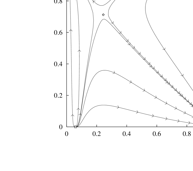
Figure 2: The RG flow projected on the compactified $(\tilde{g},\,\tilde{\gamma})$ plane ($d=1.2$, $\alpha=1$, $N=3$).

We notice the interesting fact that there exists a range of values $\alpha_{*}\leq\alpha<2$ for which one obtains a $z\equiv 1$ dynamic scaling exponent in the proximity of the quantum critical point, even in the presence of a damping term. In other words, there can be “soft” damping terms which do not spoil the spin-wave behavior of the fixed point. Within the $\epsilon$-expansion for $N=3$ $\alpha_{*}$ is given by $\alpha_{*}=3-d$ (cf. Fig. 1). We shall argue about the extension of these results to the $d=2$ case in the next subsection.

3.2 Beyond the one-loop analysis

The above analysis of the stability of FP1 vs. FP2 bears a strong similarity with the study of the $\phi^{4}$ theory with long range interactions [36, 37]. For small $\epsilon_{1}$ and $\epsilon_{2}$ one has $\alpha\simeq 2$ and $d\simeq 1$ and therefore $\eta\simeq 2-\alpha$, coherently with [36]. The two fixed points studied in [37] correspond to our FP1 and FP2; in our approach they are selected by the value of $z^{(0)}$. The continuity of $\eta$ for $\alpha\rightarrow 2$ appears as a consequence of their relative stability, as in [37]. The computations here are considerably simpler, since first-loop calculations are sufficient to establish the general picture. Another difference is in the presence of the dynamic exponent $z$, which was absent in the classical works [36, 37].

It is worth stressing the fact, noticed after Eq. (12), that the non-analyticity of the term $|\omega|^{\alpha}$ is not reproduced under renormalization, at least at first loop. As a consequence $\gamma$ does not get singular corrections by itself, but only scales according to its bare dimension and to the anomalous field dimension. The indication coming from [36, 37, 38] is that this will be true also at higher orders. This would imply that, as an exact result, $\gamma$ scales in the critical region according to the exponent

$$x_{\gamma}=2-\alpha z-\eta$$ (25)

irrespectively from the approximation. The value $z_{2}$ can then be obtained directly from the condition $x_{\gamma}=0$, giving

$$z_{2}=\frac{2-\eta}{\alpha}$$ (26)

which is in agreement with our one-loop analysis and is expected to remain valid at higher loop orders as well.

This exact relation can be used to settle the problem of the crossover from FP1 to FP2. This crossover takes place when $z_{2}=z_{1}=1$, that is, using (26), when $\alpha=\alpha_{*}\equiv 2-\eta(\alpha_{*})$, where $\eta(\alpha)$ is the anomalous field dimension for a given $\alpha$. Continuity of $\eta$ through the crossover implies $\eta(\alpha_{*})=\eta_{1}=\eta_{2}$ with $\eta_{1}$ being the critical exponent of the sigma model with zero damping in $d+1$. For twodimensional systems, like the cuprates, $d+1=3$. Numerical estimates for the critical indices of the $\mathrm{O}(3)$ symmetric $\phi^{4}$ field theory obtained from summed perturbation series at fixed dimension $3$ (see [41] and Table 25.4 of [27]) give $\eta\simeq 0.033\pm 0.004$ and $\alpha_{*}\simeq 1.966\pm 0.004$. In this respect the $\epsilon$-expansion greatly overestimates $\eta$ and underestimates $\alpha_{*}$ in $d=2$ (see Fig. 1). This suggests that, as a consequence of this small value of $\eta$, since the relation (26) is probably an exact relation, for $\alpha$ near one the physically relevant line of fixed point would be FP2.

It appears therefore that the $z=1$ behavior observed in the cuprates can be accounted for in this framework only in the hypothesis that some mechanism like the reduction of the spectral weight of low-frequency quasi-particle is so strong to effectively produce a $|\omega|^{\alpha}$ damping term with $\alpha$ very close to $2$.

4 The ordered phase: a scaling approach

In the ordered phase the effect of holes in the small-doping limit of the cuprates acts as a perturbation of the $T=0$ antiferromagnetically ordered ground state. The description of the interplay of spin and fermion degrees of freedom when approaching the QCP from the ordered side presents major difficulties. The simple introduction in the effective sigma model of a $\gamma|\omega|^{\alpha}$ term is not satisfactory, since this term would be relevant also in the proximity of the ordered critical point $g=0$, and would completely destroy the spin-wave picture of the ordered ground state.

In the ordered phase the appearance of a non-zero staggered magnetization $N_{0}$ is accompanied by the presence of two quasi-particle bands, separated by an energy $\Delta$ (for a mean field analysis see e.g. Ref. [28]). As a consequence, one would expect the decay of spin-wave excitations in particle-hole pairs to be disfavored for $|\omega|\lesssim\Delta$, and an effective damping be felt only for $|\omega|\gtrsim\Delta$. Moreover, in an AFI-PM transition $\Delta$ should vanish at the QCP as well as $N_{0}$ does. Were this not the case, since $\Delta=0$ in the disordered phase one could hardly match the critical behavior on the two sides of the transition. We are not in a condition to directly link the scale $\Delta$ to the staggered magnetization $N_{0}$ since the precise relation, if any, should emerge from the unknown microscopic dynamics of the quasiparticles. In this Section we try to get some insight in this difficult problem using simple scaling arguments. We will conjecture for $\Delta$ a scaling law with a critical exponent $y$, computable in principle from the full theory including also the fermionic degrees of freedom, and we shall try to assess the value of $y$ in a self-consistent way, once the value of $\alpha$ for the damping in the disordered phase is given. We emphasize that this procedure is not as reliable as the RG computation exposed in the preceding Sections and has an heuristic character.

A model damping term which could take into account the appearance of the scale $\Delta$ is

$$f(\omega)=\gamma\frac{|\omega|^{b}}{(\omega^{2}+\Delta^{2})^{\frac{b-\alpha}{2}}}\simeq\left\{\begin{array}[]{ccc}r|\omega|^{b}&,&|\omega|<\Delta\\ \gamma|\omega|^{\alpha}&,&|\omega|>\Delta\end{array}\right.$$ (27)

with $1\leq\alpha<2\leq b<3$, and $r=\gamma\Delta^{\alpha-b}$. We shall later assume that $\Delta$ vanishes at the QCP, so that the crossover between the two regimes is continuously shifted while approaching the transition. Here we consider $\Delta$ as a free parameter at the same level as $r$ and $\gamma$. Assuming that changing the scale, $f(\omega)$ approximately maintains the form (27) with varying values of $r$ and $\gamma$ one finds from (10) the characteristic exponents

$$x_{\gamma}=2-\eta-\alpha z,\qquad x_{r}=2-\eta-bz,\qquad x_{\Delta}=z.$$ (28)

Our phenomenological assumptions suggest that damping be relevant only at high frequencies. In this regime the spin-wave velocity $c_{\mathrm{sw}}$ goes as $c_{\mathrm{sw}}\sim s^{1-z_{2}}$ . On the other hand, at any given scale the relevant $\omega$-modes are characterized by the condition $\omega^{2}=O(1)$. So, damping is relevant up to the scale $\bar{s}$ where $\Delta$ becomes of order $1$. Beyond this scale the gap for spin-wave decay is visible and $f(\omega)$ is irrelevant. If $\Delta$ at the “microscopic” scale $s=1$ had a finite value, eventually $f(\omega)$ would be always irrelevant. The simplest way to take into account the physical condition that $\Delta$ should vanish approaching the transition is to assume that

$$\left.\Delta\right|_{s=1}\sim(g_{*}-g_{0})^{y}$$ (29)

where $g_{0}=\left.g\right|_{s=1}$ and $g_{0}\to g_{*}$. This condition encodes in a simplified, phenomenological way the complicated interaction between damping and antiferromagnetic order, mediated in the full theory by the fermionic degrees of freedom.

Taking into account (29) and the scaling exponents (28) we get

$$\bar{s}\sim(g_{*}-g_{0})^{-y/z_{2}},\qquad g_{0}\to g_{*}$$ (30)

Approximately at this scale damping becomes irrelevant and the critical behavior starts being characterized by $z=1$. This gives $c_{\mathrm{sw}}$ vanishing as

$$c_{\mathrm{sw}}\sim\bar{s}^{1-z_{2}}\sim(g_{*}-g_{0})^{y(z_{2}-1)/z_{2}},\qquad g_{0}\rightarrow g_{*}$$ (31)

For $\alpha$ not too close to two (specifically for $\alpha<\alpha_{*}$) by approaching the quantum transition from the disordered phase one observes, as already discussed, a dissipative behavior dominated by the fixed point FP2, with the scaling law $\omega\sim k^{z_{2}}$. Deep into the broken symmetry phase one instead has a propagating behavior, $\omega\sim c_{\mathrm{sw}}k$. This should match the critical behavior at the scale $\xi\sim(g_{0}-g_{*})^{-\nu}$, with $\nu$ the corresponding critical index. Continuity of the critical behavior in a neighborhood of the critical point imposes then $c_{\mathrm{sw}}\sim\xi^{1-z_{2}}$, i.e.

$$c_{\mathrm{sw}}\sim|g_{*}-g_{0}|^{\nu(z_{2}-1)},\qquad g_{0}\to g_{*}$$

This is compatible with (31) only for

$$y=\nu z_{2}$$ (32)

In terms of $\xi$ this condition on the critical behavior of the energy separation $\Delta$ gives $\delta\sim\xi^{-z_{2}}$.

5 Conclusions

It is not unreasonable to expect that the damped sigma model we considered contains some of the physics of the quantum critical point of the underdoped layered cuprates. For this reason we performed a RG analysis directly on this model, trying to maintain sufficient generality in the form of the effective damping term, in particular introducing an exponent $\alpha\geq 1$ that could account for the observed pseudogap behavior. In the broken symmetry phase we tried to get some insight on the interplay between damping and AF ordering using simple scaling arguments.

In both the ordered and the disordered phases, assuming continuity of the hydrodynamic behaviors at the quantum transition, we obtained that for $\alpha<\alpha_{*}$ (where $\alpha_{*}(d=2)$ is expected to be very close to 2) it is not possible to account for the observed $z=1$ scaling law. It was observed in Ref. [28] that the $z=1$ scaling can be recovered at higher temperatures, when typical frequencies would become larger than the $T=0$ value of the damping term. However, experimentally it is the $z=1$ behavior which is observed at lower temperatures, while a relaxational $z=2$ behavior is observed at higher $T$ [23]. It was argued [42, 23] that this could be due to the neglected $T$-dependence of the damping term $\gamma$. We propose in this paper that the same effect can be accounted for by assuming that the decay of the quasi-particle spectral weight for low frequencies produces a “soft” damping term $\sim|\omega|^{\alpha}$ with $\alpha\geq\alpha_{*}$. The $z=1$ scaling would then be a consequence of an almost linear decay of the quasi-particle spectral weight. We notice that this reduced weight is fully consistent with the observed occurrence of a pseudogap below a crossover temperature $T^{*}$ in the underdoped region of the phase diagram for the cuprates. The origin of this pseudogap might arise from extrinsic mechanisms like local Cooper-pair formation and/or stripe fluctuations. Alternatively a pseudogap could be the very consequence of the intrinsecally non Fermi liquid nature of the system [34] or of strong critical fluctuations occurring near the QCP. In this last regard singular AF fluctuations have been shown within a spin-fermion model to strongly modify the quasiparticles properties [43] in the proximity of the “hot”points of the Fermi surface separated by the AF wavevector. Since the particle-hole excitations around these points are responsible for the low-energy spin-wave decay, this naturally affects the damping of spin excitations, in a complicated interplay which deserves further investigation. We notice that the fluctuation-induced spectral weight reduction for the fermionic excitations is a definite signature of a non-Fermi liquid metallic state. This is in agreement with general arguments put forward by Anderson (see e.g., Ref. [44]) on the difficulty in continuously connecting a charge-gapped insulating phase with a normal Fermi-liquid phase. We remark, however, that Anderson’s arguments extend the presence of a non-Fermi-liquid phase all over the metallic state as a consequence of low dimensionality. On the other hand, within the QCP scenario, the violation of the Fermi-liquid properties is a consequence of critical fluctuations, which are only present around the critical point. As soon as one moves away from this point, the fluctuations loose their critical character thus providing simple perturbative corrections to the Fermi liquid state.

It is worth noting that the analysis carried out in this paper is not only related to the superconducting cuprates, but it has connections with other physically interesting problems, like the spin chains with long range interaction and macroscopic quantum tunnelling. By considering the model (2) in $d=0$, it is seen that the frequency axis is left as the only relevant “direction” (cf. the technical considerations presented in Appendix A). As a first consequence, all the critical behavior should be reformulated in terms of frequency by suitably rescaling of the critical indices by $1/z$. The frequency axis becomes then equivalent to a single space direction, via the dynamic critical index $z$, thus establishing a connection with onedimensional classical models. Fourier transforming back to (imaginary) times the damping term in (2) gives rise to a long range interaction of the type $|t-t^{\prime}|^{-1-\alpha}$. Our results can be directly extended to the case $0<\alpha<1$. This leads to the comparison with the onedimensional (classical) $N$-component spin model with long-range interaction considered in Ref. [45]. One can recognize that, once the spatial term is dropped in (2) the connection is established through the coupling combinations $\gamma/g$ and $gc^{2}$. This allows to rewrite the RG equation for $g/\gamma$ in the same form as Eq. (7) of Ref. [45], with $g/\gamma$ (to be identified with $T$) having a fixed point (FP2 in our model) and $(1/gc^{2})_{*}=0$.

Whitin the $d=0$ case, $N=2$ deserves special attention because of the connection with macroscopic quantum tunnelling [46, 47]. This connection is realized by observing that the $\mathrm{O}(2)$ non-linear $\sigma$ model can be rewritten in terms of an angular degree of freedom and that the addition of the magnetic field produces a cos-like interaction (sine-Gordon model). In $d=0$ the model then describes a single degree of freedom with a kinetic ($\omega^{2}$) term in a multivalley potential. In the presence of dissipation, a linear-in-frequency term can appear, leading again to long-range interactions on the (imaginary) time axis. Models of this kind were considered by Chakravarty [48] in the case of a double well potential and successively by Schmid [49] to describe a dissipative quantum particle in a onedimensional periodic potential. In particular, the only difference between our Eq. (2) at $N=2$ and this latter model is the non-periodicity of the dissipative term of Ref. [49].

In the model of Schmid, for vanishing $h$ ($g=0$ in his notation), a line of fixed points for $\eta$ (corresponding to our $\gamma/g$) was found, with a critical point $\eta_{c}$ separating a regime with relevant $h$ from one with irrelevant $h$. The long-range term introduced in [49] is quadratic in the fields, so that the model for $h=0$ is free and $\eta$ (i.e. $\gamma/g$) does not renormalize. A (dual) fixed point was also found for very large $h$, where the model of Ref. [49] was stated to be equivalent to the one of Ref. [48]. We observe that, differently from the model of Ref. [49] our long-range term mantains the periodicity in the angular variable and provides an interaction. This renormalizes the coupling, thus allowing $\gamma/g$ to flow under renormalization even at $h=0$. One could conjecture that a new fixed point arises at finite $h$. An adequate analysis would require a RG study at finite $h$ going beyond the $\epsilon$-expansion and taking into account instantonic corrections. This is an interesting open problem which deserves further investigation.

Acknowledgments: We gratefully acknowledge interesting discussions with C. Di Castro, A. Chubukov and I. Kolokolov.

Appendix A Computation of the critical indices

For the computation of the eigenvalues $\omega^{\mathrm{R}},\,\omega^{\mathrm{A}}$ of the linearization of the RG transformation (18-20) in the point FP2 it is convenient to rewrite it in the form (22-24). The secular equation is found to depend on

$$\mathcal{I}_{\alpha}=\left.u\frac{d}{du}\log\tilde{I}_{\alpha}(u)\right|_{u=u_{*}},\quad\mathcal{K}_{\alpha}=\left.u\frac{d}{du}\log\tilde{K}_{\alpha}(u)\right|_{u=u_{*}}$$ (33)

with $u=\tilde{\gamma}\equiv c^{\alpha}\gamma$ and $\tilde{I}_{\alpha}$ and $\tilde{K}_{\alpha}$ given after Eq. (21). For $\epsilon=d-2+2/\alpha\rightarrow 0$ one has $u_{*}\rightarrow+\infty$, and in this limit it is easy to derive from (16,17), for $\alpha>1$:

$$\tilde{I}_{\alpha}(u)\simeq\frac{S_{d}}{(2\pi)^{d+1}}\frac{2\pi}{\alpha\sin\frac{\pi}{\alpha}}u^{-1/\alpha},~{}~{}~{}~{}\tilde{K}_{\alpha}(u)\simeq\frac{S_{d}}{(2\pi)^{d+1}}\frac{\pi(\alpha-1)}{2\sin\frac{\pi}{\alpha}}u^{1/\alpha}$$

which substituted in (33) gives

$$\mathcal{I}_{\alpha}\simeq-\frac{1}{\alpha},\quad\mathcal{K}_{\alpha}\simeq\frac{1}{\alpha}$$ (34)

Solving (21) asymptotically for $u_{*}\rightarrow+\infty$ ($\epsilon\rightarrow 0$) and fixed $\gamma_{*}$ gives

$$u_{*}^{2}\simeq\left\{\frac{4[(N-2)\alpha+1](2-\alpha)}{\alpha^{3}(\alpha-1)}\right\}^{\alpha}\frac{1}{\epsilon^{\alpha}},~{}~{}~{}~{}c_{*}\sim\frac{1}{\sqrt{\epsilon}}$$

Using (34) one easily finds $\omega_{2}^{\mathrm{R}},\,\omega^{\mathrm{A}}_{2}$ at first order in $\epsilon$.

For $\alpha\rightarrow 1$ the expressions (16,17) reduce to

$$I_{1}(c,\gamma) = \frac{S_{d}}{(2\pi)^{d+1}}\left\{\begin{array}[]{lll}\frac{4c}{\sqrt{4-(c\gamma)^{2}}}\arctan\frac{\sqrt{4-(c\gamma)^{2}}}{(c\gamma)}&,&0<c\gamma<2\\ \frac{2c}{\sqrt{(c\gamma)^{2}-4}}\log\frac{c\gamma+\sqrt{(c\gamma)^{2}-4}}{c\gamma-\sqrt{(c\gamma)^{2}-4}}&,&c\gamma>2\end{array}\right.$$ (37)

$$K_{1}(c,\gamma) = \frac{S_{d}}{(2\pi)^{d+1}}\frac{\gamma}{2}$$ (38)

The same expressions can be obtained by a direct evaluation of (7, 13) for $\alpha=1$. In particular the original expression (7) shows that $I_{1}$ is in fact an analytic function of $c$ and $\gamma$. However, some problems arise when using expressions (37) and (38) to compute critical indices directly for $\alpha=1$ instead of considering the $\alpha\to 1$ limit of the general expressions given in Section 3.1. For $\alpha=1$ in fact one expands around the critical dimension $d_{\mathrm{c}}=0$ and the factor $S_{d}$ coming from angular integration vanishes. If the same computation is performed using field-theoretical methods, instead of Wilson’s integration on the momentum shell, no such problems arise: e.g. one has

$$\int\frac{\,\mathrm{d}\omega\,\mathrm{d}^{d}k}{k^{2}+\omega^{2}/c^{2}+\gamma\omega^{\alpha}}=\frac{2}{2-\alpha}\frac{\pi/2}{\sin\frac{\pi d}{2}}\frac{2\pi^{d/2}}{\Gamma(\frac{d}{2})}\frac{\Gamma\left(\frac{1-d}{2-\alpha}\right)\Gamma\left(\frac{\alpha\epsilon}{2(2-\alpha)}\right)}{\Gamma\left(1-\frac{d}{2}\right)}c^{\frac{\alpha\epsilon}{2-\alpha}}\gamma^{\frac{d-1}{2-\alpha}}$$ (39)

which correctly behaves as $\epsilon^{-1}$ for $\epsilon\rightarrow 0$, independently of the value of $\alpha$. Notice that the $\Gamma^{-1}(d/2)$ factor coming from $S_{d}$ is cancelled by the factor $\left(\sin(d\pi/2)\right)^{-1}$ and the $\epsilon^{-1}$ divergence arises from $\Gamma(\alpha\epsilon/2(2-\alpha))$. The problems with the Wilson method are resolved if one makes a more symmetric choice of the integration shell, e.g. integrating over all the $\boldsymbol{\pi}_{\boldsymbol{k},\omega}$ with $e^{-l}<\sqrt{k^{2}+\omega^{2}}<1$ (which implies introducing a frequency cutoff). With this choice $I_{\alpha}$ is finite for $d\rightarrow 0$. We observed that $I_{\alpha},\,K_{\alpha}$ computed with either choice of cutoffs have the same $c,\,\gamma$ dependence, the only effect of the choice of the symmetric shell being that the integrals do not vanish for $d\rightarrow 0$. In particular, the expressions for $\omega_{2}^{\mathrm{R}}$, $\omega_{2}^{\mathrm{A}}$ given in the text are valid for $1\leq\alpha<2$: as a matter of fact, they are computed from the values (34), which do not contain the angular integration factor $S_{d}$.

References

- [1] For a review on magnetism in the cuprates see: a) D. C. Johnston, Handbook of Magnetic Materials, Vol. 10 p. 1-237, edited by K. H. J. Buschow (North Holland, Amsterdam 1997), and b) C. Berthier, M. H. Julien, M. Horvatić, and Y. Berthier, J. de Phys. I 6 (1996) 2205.
- [2] For a recent review on magnetism in the cuprates with a particular attention to NMR-NQR experiments see: A. Rigamonti, F. Borsa and P. Carretta, Basic aspects and main results of NMR-NQR spectroscopies in high temperature superconductors, preprint 1998.
- [3] P. W. Anderson, Science 235 (1987) 1196.
- [4] V. J. Emery, S. A. Kivelson, and H. Q. Lin, Phys. Rev. Lett. 64 (1990) 475; M. Marder, N. Papanicolau, and G. C. Psaltakis, Phys. Rev. B 41 (1990) 6920.
- [5] V. J. Emery and S. A. Kivelson, Physica C 209 (1993) 597.
- [6] C. Castellani, C. Di Castro, and M. Grilli, Z. Phys. B 103 (1997) 137.
- [7] I. Affleck and B. Halperin, J. Phys. A 29 (1996) 2627.
- [8] A. H. Castro Neto and D. Hone, Phys. Rev. Lett. 76 (1996) 2165.
- [9] J. H. Cho, F. Borsa, D. C. Johnston, and D. R. Torgeson, Phys. Rev. B 46 (1992) 3179.
- [10] F. C. Chou et al., Phys. Rev. Lett. 75 (1995) 2204.
- [11] R. J. Gooding, N. M. Salem, and A. Mailhot, Phys. Rev. B 49 (1994) 6067, and references therein.
- [12] I. Ya. Korenblit, V. Cherepanov, A. Aharony, O. Entin-Wohlman, cond-mat/9709056.
- [13] S. Chakravarty, B. I. Halperin, and D. R. Nelson, Phys. Rev. B 39 (1989) 2344.
- [14] S. Sachdev and J. Ye, Phys. Rev. Lett. 69 (1992) 2411.
- [15] A. V. Chubukov and S. Sachdev, Phys. Rev. Lett 71 (1993) 169; Phys. Rev. Lett 71 (1993) 2680(E);
- [16] A. V. Chubukov, S. Sachdev, and J. Ye, Phys. Rev. B 49 (1994) 11919.
- [17] A. Sokol and D. Pines, Phys. Rev. Lett. 71 (1993) 2813.
- [18] A. Sokol, in The Los Alamos Symposium 1993 – Strongly Correlated Electronic Materials, edited by K. S. Bedell et al. (Addison-Wesley, Reading, MA, 1994), pp. 490–493.
- [19] T. Imai, C. P. Slichter, K. Yoshimura, and K. Kosuge, Phys. Rev. Lett. 70 (1993) 1002.
- [20] M. Takigawa, Phys. Rev. B 49 (1994) 4158.
- [21] V. Barzykin, D. Pines, A. Sokol, and D. Thelen, Phys. Rev. B 49 (1994) 1544.
- [22] V. Barzykin and D. Pines, Phys. Rev. B 52 (1995) 13585.
- [23] A. V. Chubukov, D. Pines, and B. P. Stojković, J. of Phys. 8 (1996) 10017.
- [24] F. D. M. Haldane, Phys. Lett. 93A (1983) 464; Phys. Rev. Lett. 50 (1983) 1153; I. Affleck, Nucl. Phys. B257 (1985) 397.
- [25] A. M. Polyakov, Phys. Lett. 59B (1975) 79.
- [26] E. Brézin and J. Zinn-Justin, Phys. Rev. B 14 (1977) 3110.
- [27] J. Zinn-Justin, Quantum Field Theory and Critical Phenomena (Oxford University Press, New York, 1993).
- [28] S. Sachdev, A. V. Chubukov, and A. Sokol, Phys. Rev. B 51 (1995) 14874.
- [29] B. I. Shraiman and E. D. Siggia, Phys. Rev. Lett. 61, (1988) 467; Phys. Rev. B 42 (1990) 2485.
- [30] S. Sachdev, Phys. Rev. B 49 (1994) 6770.
- [31] J. A. Hertz, Phys. Rev. B 14 (1976) 1165.
- [32] M. Randeria and J.-C. Campuzano, in Proceedings of the International School of Physics “Enrico Fermi” (Varenna, 1997).
- [33] A. V. Chubukov, D. K. Morr, and K. A. Shakhnovich, Phyl. Mag. B 74 (1996) 563.
- [34] P. W. Anderson, Phys. Rev. Lett. 64, 1839 (1990); ibid. 65, 2306 (1990)
- [35] J. Maly and K. Levin, Phys. Rev. B 55, R15657 (1996).
- [36] M. E. Fisher, S. Ma, and B. G. Nickel, Phys. Rev. Lett. 29 (1972) 917.
- [37] J. Sak, Phys. Rev. B 8 (1973) 281.
- [38] A. Aharony, in Phase Transitions and Critical Phenomena, edited by C. Domb and M. S. Green (Academic Press, 1976), vol. 6, p. 358.
- [39] A. V. Chubukov, Phys. Rev. B 52 (1995) R3840.
- [40] D. R. Nelson and R. A. Pelcovits, Phys. Rev. B 16 (1977) 2191.
- [41] J. C. Le Guillou and J. Zinn-Justin, Phys. Rev. Lett. 39 (1977) 95; Phys. Rev. B 21 (1980) 3976.
- [42] P. Monthoux and D. Pines, Phys. Rev. B 49 (1994) 4261.
- [43] R. Hlubina and T. M. Rice, Phys. Rev. B 51 (1995) 9253.
- [44] G. Baskaran and P. W. Anderson, cond-mat/9706076.
- [45] J. M. Kosterlitz, Phys. Rev. Lett. 37 (1976) 1577.
- [46] A. O. Caldeira and A. J. Legget, Phys. Rev. Lett. 46, (1981) 211.
- [47] The case and describes phase fluctuations in low dimensional superconductors. RG analyses on models, which are slightly different from the one considered in the present paper have been carried out by S. Chakravarty, et al., Phys. Rev. B 37, (1988) 3283, V. J. Emery and S. A. Kivelson, Phys. Rev. Lett. 74, (1995) 3253, and, more recently, by M. V. Feigel’man and A. I. Larkin, cond-mat/9803006.
- [48] S. Chakravarty, Phys. Rev. Lett. 49 (1982) 681.
- [49] A. Schmid, Phys. Rev. Lett. 51 (1983) 1506.