Scaling in the time-dependent failure of a fiber bundle with local load sharing

Abstract

We study the scaling behaviors of a time-dependent fiber-bundle model with local load sharing. Upon approaching the complete failure of the bundle, the breaking rate of fibers diverges according to $r(t)\propto(T_{f}-t)^{-\xi}$, where $T_{f}$ is the lifetime of the bundle, and $\xi\approx 1.0$ is a quite universal scaling exponent. The average lifetime of the bundle $<T_{f}>$ scales with the system size as $N^{-\delta}$, where $\delta$ depends on the distribution of individual fiber as well as the breakdown rule.

PACS numbers: 64.60.Fr, 62.20.Mk, 64.60.Ak, 05.45.+b

I Introduction

The failure of disordered materials under load is a complicated phenomenon, the modelling of which is a subject of great interest because it forms the basis of numerous applications from space technology to paper making [2]. The failure process also represents an important class of pattern formation and scaling problems [3]. The fiber-bundle model, as a simple and interesting theoretical model in this field, has been studied extensively. The early studies on the static fiber-bundle model might be traced back to the work by Daniels [4], while the time-dependent method to the model was proposed by Coleman [5]. In a recent paper [6], Gomez et al developed a probabilistic method for solving the time-dependent model. In the static model, each fiber in the bundle is assumed to have a strength threshold, a load above which will break it instantly, while a load below which does no harm. In the time-dependent model, each fiber is assumed to have a lifetime under a given load history, and it breaks because of fatigue. The load-sharing rules, which describe how the load of a broken element is transferred to survival elements, are essential to the definition of the model. In what is called Equal Load Sharing (ELS) model, the total load of the bundle is equally shared by all survival fibers, while in the Local Load Sharing (LLS) model the load of a broken fiber is transferred to its nearest neighbors. Hierarchically organized fiber bundle was also proposed, and has received much attention especially in the geophysical literature [7, 8]. Various aspects of the fiber-bundle model have been investigated, such as the strength distribution for static model [4, 9] and the lifetime distribution for dynamic one [5, 10]. In this paper, we will study an LLS time-dependent model, and investigate the scaling behaviors in its breaking process.

Let us consider a fiber bundle consisting of $N$ fibers. We assume that when a fiber is subjected to a load history $\sigma(t)$, some damage will accumulate, which is described by

$$d(t)=\int_{0}^{t}\nu[\sigma(\tau)]d\,\tau,$$ (1)

where the load-dependent $\nu(\sigma)$ is introduced as a hazard rate, which is usually referred to as breakdown rule [5] in the literature.

A fiber, say fiber $i$, is assumed to have an endurance threshold (or say, critical damage) $d_{i}^{c}$, which is drawn from a cumulative distribution

$$P(d_{i}^{c}<d)=1-\exp\left[-\Psi(d)\right],$$ (2)

where $\Psi(x)$ is the shape function. Previous theoretical and experimental work [5, 10] favors a shape function of the form

$$\Psi(x)=x^{\beta}.$$ (3)

As for the breakdown rule $\nu(\sigma)$, two special forms are widely used in the literature: the power-law form

$$\nu_{p}(\sigma)=\nu_{0}\left({\sigma\over\sigma_{0}}\right)^{\rho},$$ (4)

and the exponential form

$$\nu_{e}(\sigma)=\phi_{0}\exp\left({\eta\sigma\over\sigma_{0}}\right),$$ (5)

with $\nu_{0}$, $\sigma_{0}$, $\rho$, $\phi_{0}$, $\eta$ all positive constants.

Under load each fiber will break when the damage accumulated exceeds its endurance threshold, and all fibers will break eventually, leading to the complete failure of the bundle. Let us denote the total load on the bundle by $N\sigma$. In general, $\sigma$ is a function of time. For example, it can be a linearly increasing function or a periodic function of time [5]. In this paper, we will consider the simple case that $\sigma$ is a constant. In the following numerical calculations, if not otherwise specified, the load is set to be $\sigma=\sigma_{0}$. It should be noted that although the total load on the bundle is constant, the loads on the individual fibers $\sigma_{i}(t)$’s are not.

II The LLS model

We consider a fiber-bundle model with the LLS rule. $N$ fibers are arranged evenly on a circle, and each of them has two adjacent neighbors. The total load on the bundle $N\sigma$, kept constant in this study, is shared by survival fibers. A survival fiber $i$ carries the load $\sigma_{i}=K_{i}\sigma$, where the concentration factor $K_{i}=1+(l_{i}+r_{i})/2$. Here $l_{i}$ ( $r_{i}$ ) is the number of broken fibers on the left (right) of fiber $i$. It is clear that $\sum_{i}K_{i}=N$, so the total load is conserved. With such a load sharing rule, the load of a broken fiber is transferred to the survival neighbors on both sides. Note that this rule is different from the one-side case [11], in which the load of a broken fiber is transferred only to its neighbor on one side.

This LLS fiber-bundle model was in early years developed by Harlow and Phoenix[9] to model the failure of a unidirectional composite material under tensile loads. The model has ever since drawn much attention of many authors. In recent years, the static LLS fiber-bundle model was studied in terms of the burst-size distribution [12, 13, 14] and the failure probability of the bundle under a given load [15, 16]. In this study, we will focus on the scaling behaviors of this dynamic LLS fiber-bundle model.

III Scaling of Breaking Rate with Time to Failure

Let $N_{f}(t)$ be the number of broken fibers in the bundle at time $t$, with $N_{f}(0)=0$ and $N_{f}(T_{f})=N$, where $T_{f}$ is the lifetime of the whole bundle. The breaking rate of the bundle is defined as

$$r(t)={\delta N_{f}(t)\over\delta t}$$ (6)

We have performed extensive Monte Carlo simulations of the breaking process of the time-dependent fiber-bundle model with LLS, and found that in a wide range of parameter value the breaking rate $r(t)$, upon approaching the complete failure, scales with the time to failure as

$$r(t)\propto(T_{f}-t)^{-\xi}$$ (7)

and the scaling exponent $\xi\approx 1.0$ is of a quite universal value. Examples of the behavior of the breaking rate are shown in Fig. 1. In this log-log plot, dashed lines with slope $-1$ are also shown for reference. The numerical results are not very smooth because of fluctuation, but the general trend of the breaking rate $r(t)$ agrees well with Eq.(7).

In what follows, we try to understand the scaling behavior (7) through analytical treatment. In the discussion, we take the limit $N\rightarrow\infty$. Let us call the connective broken fibers bounded by unbroken ones as a crack. The size of a crack is the number of broken fibers. Because of the local load-sharing rule, the fibers bounding a larger crack experience heavier load than those bounding smaller ones. So when a major crack is formed in the bundle, breaking will mostly occur along it. In other words, it is the fibers adjacent to the major crack that will most probably break in the next step. This can be seen from the evolution of the size $c_{m}$ of the biggest crack. Fig. 2 shows $c_{m}$ versus the total number of broken fibers in the bundle. At the early stage of the failure process, $c_{m}$ remains constant for some time ( $A$ ), which indicates that small cracks nucleate at different locations. As more and more fibers break, some small cracks will coalesce or grow to form a major crack, and then the major crack grows, which is reflected in this figure by a linear increase of $c_{m}$ with $N_{f}$ with slope $1$ ( $B$ ). During its growth, the major crack may also coalesce with some small cracks and become even larger, indicated in the figure by local slopes steeper than $1$ at some points ( e.g., $C$ ).

Suppose the size of the major crack is $N_{f}(t)-k$, where $k$ is the number of failed fibers which do not belong to the major crack. The loads on the fibers adjacent to the major crack are $[1+(N_{f}-k)/2]\sigma$, so damage will accumulate in these fibers with the rate $\nu([1+(N_{f}-k)/2]\sigma)$. The breaking rate of these fibers can be assumed to be proportional to $\nu(\cdot)$, and one has

$$r(t)={d\,N_{f}(t)\over d\,t}=A(t)\nu\left(\left[1+\frac{N_{f}-k}{2}\right]\sigma\right),$$ (8)

where $A(t)$ is a factor that depends on the accumulated damages in the fibers and their endurance thresholds. An exact calculation of $A(t)$ is extremely difficult and might be impossible. We assume that the variance of $A(t)$ is unimportant and take $A$ as a constant for simplicity. The validity of this assumption is verified by the agreement with numerical results. Note that sometimes a fiber adjacent to the major crack happen to be also adjacent to a small crack, resulting in a little more load on it, the influence of which on the breaking rate however, is negligible upon approaching the complete failure.

For the exponential form of breakdown rule (5), we have

$${d\,N_{f}(t)\over d\,t}=A\phi_{0}\exp\left[\eta\left(1+{N_{f}-k\over 2}\right){\sigma\over\sigma_{0}}\right],$$ (9)

and therefore,

$$r(t)=\alpha^{-1}(T_{f}-t)^{-1},$$ (10)

where $\alpha=\eta\sigma/(2\sigma_{0})$, $T_{f}$ is the value of time that gives $N_{f}(T_{f})\rightarrow\infty$.

For the power-law form of breakdown rules (4),

$${d\,N_{f}(t)\over d\,t}=A\nu_{0}\left[\left(1+{N_{f}-k\over 2}\right){\sigma\over\sigma_{0}}\right]^{\rho},$$ (11)

and

$$r(t)=C\left[{\rho-1\over 2}C(T_{f}-t)\right]^{\rho\over 1-\rho}\propto(T_{f}-t)^{-1-{1\over\rho-1}}$$ (12)

with $C=A\nu_{0}(\sigma/\sigma_{0})^{\rho}$, and $N_{f}(T_{f})\rightarrow\infty$. So $\xi=1+1/(\rho-1)$. Since $\rho$ is of quite large value, typically between $10$ and $80$ [10], it is not surprising that $\xi\approx 1.0$ in the numerical simulations.

IV Lifetime of the bundle

In deducing the scaling of the breaking rate, we have taken the thermodynamic limit by setting $N_{f}(T_{f})=\infty$. In numerical simulations however, we cannot realize infinite system size. Given the local load-sharing rule, the lifetime $T_{f}$ of a fiber bundle depends on the endurance of each fiber. Due to fluctuation, $T_{f}$ is different from bundle to bundle. Since the fluctuation is related to the system size, the average lifetime $<T_{f}>$ of the bundle should in principle depend on $N$, which is known as size effect. We found that in general the average life time $<T_{f}>$ scales with the system size as

$$<T_{f}>\propto N^{-\delta},$$ (13)

where $<\cdots>$ means the ensemble average. Some of the numerical results are shown in Fig. 3, in which the power-law fit to the data is quite good. Some other forms of fit to the data were also tried, but none of them is better than the power law. It should be noted that in the static LLS model the average strength of the bundle follows a logarithmic dependence on the system size [11, 17].

The exponent $\delta$ for the power law, however, is not of a universal value. It depends on the breakdown rule as well as the distribution of damage endurance for individual fiber. We performed extensive numerical simulations to explore the relation between the exponent $\delta$ and the parameters $\beta$, $\rho$ and $\eta$. Some results are listed in Table I. There seems no simple general expression relating $\delta$ to $\beta$, $\rho$, and $\eta$. For some limiting cases, however, we can get a simple relation. From Table I, one can see that when $\rho$ or $\eta$ is large, the value of the exponent $\delta$ is very close to $1/\beta$. This result can be understood by the lifetime distribution of the fiber bundle. When $\rho$ or $\eta$ is large, the fiber bundle breaks in the following way: when the weakest fiber breaks, it will form the crack that leads to the failure of the whole bundle. So the lifetime of the bundle will be expended mostly in the weakest fiber, and is thus determined by it. From Eqs. (1), (2) and (3), the lifetime of an individual fiber under a constant load $\sigma$, is distributed as

$$P(t_{f}<t)=1-e^{-[\nu(\sigma)t]^{\beta}}.$$ (14)

For a bundle of $N$ fibers, if the bundle’s lifetime is determined by the lifetime of its weakest element, the lifetime distribution for such a bundle is, by the weakest-link rule and when $N$ is large,

$$P(T_{f}<t)=1-e^{-N[\nu(\sigma)t]^{\beta}}.$$ (15)

And this is the Webull distribution, with which the average lifetime of the bundle is

$$<T_{f}>=\int_{0}^{\infty}t\,dP(T_{f}<t)=\int_{0}^{\infty}t\,d(1-e^{-N[\nu(\sigma)t]^{\beta}}).$$ (16)

Changing the variable of integration $Nt^{\beta}=\tau^{\beta}$, one gets

$$<T_{f}>=N^{-1/\beta}\int_{0}^{\infty}\tau\,d(1-e^{-[\nu(\sigma)\tau]^{\beta}}).$$ (17)

The integration in the above equation is independent of $N$, so $<T_{f}>\propto N^{-1/\beta}$, and $\delta=1/\beta$.

From the numerical results, we notice that $\delta=1/\beta$ is not satisfied by all values of $\rho$ and $\eta$. The deviation of $\delta$ from $1/\beta$ may indicate the deviation of the lifetime distribution from the Webull distribution. In Fig. 4, we plot the lifetime distribution of the fiber bundle with Webull axes, that is, to plot $\ln\{-\ln[1-P(t)]\}$ versus $\ln t$. If the distribution is of Webull form, $P(t)=1-\exp(-at^{m})$, one should see a straight line in such a plot, and the slope of the line gives the Webull modulus $m$. For the case $\beta=2$ and $\rho=40$ (Fig. 4.b), we get a quite straight line, and the best linear fit to the distribution curve gives the Webull modulus $m\approx 2.03$, very close to $\beta=2$. Notice that for this case $\delta\approx 0.50=1/\beta$. For the case $\beta=1$ and $\rho=10$ (Fig. 4.a), however, the distribution curve is not a straight line, indicating that the lifetime is not very well Webull distributed. For this case $\delta\approx 0.49$, which is quite different from $1/\beta=1.0$.

In the early studies on the lifetime distribution, Phoenix and his collaborators  [10] were able to obtain an approximation to the lifetime distribution of the fiber bundle, which was also of Webull form. Their results were based on the idea that whenever a crack of critical size, called $k^{*}$-crack in their paper, emerges in the system, the bundle will fail instantly.

V Conclusions

In conclusion, we have studied some scaling behaviors of the time-dependent fiber-bundle model with LLS rule. In a quite wide range of parameter value, the breaking rate scales with the time to failure as $(T_{f}-t)^{-1}$. The average lifetime of the bundle scales with system size as $N^{-\delta}$, with $\delta$ dependent on the breakdown rule and endurance distribution of individual fiber. In the limiting cases that $\rho$ or $\eta$ is very large, the lifetime distribution of the bundle can be well approximated by a Webull form, and the Webull modulus for this distribution is just the shape-function parameter $\beta$, and the scaling exponent $\delta=1/\beta$.

ACKNOWLEDGMENTS

The author thanks R. B. Liu for critical readings of the manuscript. This work is supported by the National Nature Science Foundation of China, the Educational Committee of the State Council through the Foundation of Doctoral Training.

FIG. 1.: The breaking rate $r(t)$, defined in the text, scales with the time to failure as $(T_{f}-t)^{-\xi}$, where $\xi\approx 1.0$ is a quite universal value. (a) Using the power-law breakdown rule (4) with $\rho=10$, and the shape function (3) with $\beta=2$. (b) Using the exponential breakdown rule (5) with $\eta=1.0$, and shape-function parameter $\beta=4$. In both (a) and (b), the system sizes are $N=100$, and the dashed lines show the curves for $y\propto x^{-1}$ for reference.

FIG. 2.: An example of the evolution of the biggest crack in the failure process of the fiber bundle. The exponential breakdown rule is used with $\eta=1$. The other parameters are $N=100$, $\beta=4$. (b) is a part of (a) enlarged.

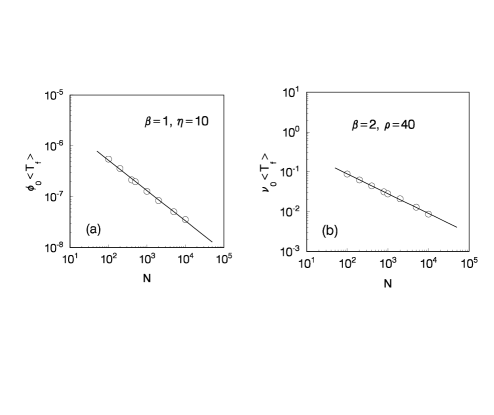
FIG. 3.: The average lifetime of the bundle scales with system size $N$ according to a power law. The circles are results from numerical simulations with at least $100$ samples, the solid line is for the power-law fit $y=ax^{-\delta}$ to the numerical data. (a) $\beta=1$, $\eta=10$, $a=8.14\times 10^{-6}$, $\delta=0.60$. (b) $\beta=2$, $\rho=40$, $a=0.87$, $\delta=0.50$.

FIG. 4.: The lifetime distribution of the LLS fiber bundle. The results in this figure are from simulations of $10^{4}$ samples. (a) $\beta=1$, $\rho=10$, $N=1000$. The curve is not a straight line. (b) $\beta=2$, $\rho=40$, $N=800$. The curve is a quite straight line, indicating a Webull distribution $P(t)=1-\exp(-at^{m})$. The best linear fit to the numerical data in (b) gives the slope $m\approx 2.03$.

TABLE I.: The exponent $\delta$, defined in Eq.(13), depends on the breakdown rule as well as the endurance distribution of the fibers.

	$\rho=10$	$\rho=20$	$\rho=40$	$\eta=1$	$\eta=10$	$\eta=20$
$\beta=1$	$0.49$	$0.83$	$0.97$	$0.17$	$0.60$	$0.97$
$\beta=2$	$0.33$	$0.47$	$0.50$	$0.10$	$0.42$	$0.52$
$\beta=4$	$0.23$	$0.26$	$0.27$	$0.053$	$0.23$	$0.26$

REFERENCES

- [1] Electronic address: zhangsd@bnu.edu.cn
- [2] Statistical Models for the Fracture of Disordered Media, edited by H. J. Hermann and S. Roux (North-Holland, Amsterdam, 1990), and references therein.
- [3] W. I. Newman, A. M. Gabrielov, T. A. Durand, S. L. Phoenix, and D. L. Turcotte, Physica D 77, 200 (1994).
- [4] H. E. Daniels, Proc. Roy. Soc. A 183, 404 (1945).
- [5] B. D. Coleman, J. Appl. Phys. 29, 968 (1958).
- [6] J. B. Gomez, Y. Moreno, and A. F. Pacheo, Phys. Rev. E 58, 1528 (1998).
- [7] W. I. Newman, D. L. Turcotte, and A. M. Gabrielov, Phys. Rev. E 52, 4827 (1995).
- [8] D. L. Turcotte, Fractals and Chaos in Geology and Geophysics. 2nd Edition, Cambridge University Press (1997).
- [9] D. G. Harlow and S. L. Phoenix, J. Composite Mater. 12, 195 (1978); ibid 12, 314 (1978).
- [10] S. L. Phoenix and L. J. Tierney, Eng. Fracture Mech. 18, 193 (1983).
- [11] J. B. Gomez, D. Iniguez, and A. F. Pacheo, Phys. Rev. Lett. 71, 380 (1993).
- [12] A. Hansen and P. C. Hemmer, Phys. Lett. A 184, 394 (1994).
- [13] S. D. Zhang and E. J. Ding, J. Phys. A 28, 4323 (1995).
- [14] M. Kloster, A. Hansen, and P. C. Hemmer, Phys. Rev. E 56, 2616 (1997).
- [15] P. L. Leath and P. M. Duxbury, Phys. Rev. B 49, 14905 (1994).
- [16] S. D. Zhang and E. J. Ding, Phys. Rev. B 53, 646 (1996).
- [17] S. D. Zhang and E. J. Ding, Phys. Lett. A 193, 425 (1994).