Electron transport through a circular constriction

Abstract

We calculate the conductance of a circular constriction of radius $a$ in an insulating diaphragm which separates two conducting half-spaces characterized by the mean free path $\ell$. Using the Boltzmann equation we obtain an answer for all values of the ratio $\ell/a$. Our exact result interpolates between the Maxwell conductance in diffusive ($\ell\ll a$) and the Sharvin conductance in ballistic ($\ell\gg a$) transport regime. Following the earlier approach of Wexler we find the explicit form of the Green’s function for the linearized Boltzmann operator. The formula for the conductance deviates by less than $11\%$ from the naive interpolation formula obtained by adding resistances in the diffusive and the ballistic regime.

I Introduction

The problem of electron transport through an orifice (also known as a point contact) in an insulating diaphragm separating two large conductors (Fig. 1) has been studied for more than a century. Maxwell [1] found the resistance in the diffusive regime when the characteristic dimension $a$ (radius of the orifice) is much larger than the mean free path $\ell$. Maxwell’s answer, obtained from the solution of Poisson equation and Ohm’s law, is

$$R_{M}=\frac{\rho}{2a},$$ (1)

where $\rho$ is resistivity of the conductor on each side of the diaphragm. Later on, Sharvin [2] calculated the resistance in the ballistic regime ($\ell\gg a$)

$$R_{S}=\frac{4\rho\ell}{3A}=\left(\frac{2e^{2}}{h}\frac{k_{F}^{2}A}{4\pi}\right)^{-1},$$ (2)

where A is the area of the orifice.

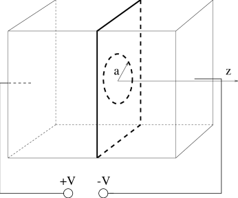
FIG. 1.: Electron transport through the circular constriction in an insulating diaphragm separating two conducting half-spaces (each with a mean free path $\ell$).

This “contact resistance” persists even for the ideal conductors (no scattering) and has a purely geometrical origin, because only a finite current can flow through a finite size orifice for a given voltage. In the Landauer-Büttiker transmission formalism [3], we can think of a reflection when a large number of transverse propagating modes in the reservoirs matches a small number of propagating modes in the orifice. In the intermediate regime, when $a\simeq\ell$, the crossover from $R_{M}$ to $R_{S}$ was studied by Wexler [4] using the Boltzmann equation in a relaxation time approximation. The influence of inelastic collisions on the orifice current-voltage characteristics was studied using classical kinetic equations in Ref. [5] and quantum kinetic equations (Keldysh formalism) in Ref. [6]. This effect underlies an experimental technique for the extraction of the phonon density of states from the nonlinear current-voltage characteristics (point contact spectroscopy [7]). Recently, the size of orifice has been shrunk to $a\simeq\lambda_{F}$ allowing the observation of quantum-size effects on the conductance [8, 9]. In the case of a tapered orifice on each side of a short constriction between reservoirs, discrete transverse states (“quantum channels”) below the Fermi energy which can propagate through the orifice give rise to a quantum version of Eq. (2). The quantum point contact conductance is equal to an integer number of conductance quanta $2e^{2}/h$.

Here we report a semiclassical treatment using the Boltzmann equation. Bloch-wave propagation and Fermi-Dirac statistics are included, but quantum interference effects are neglected. Electrons are scattered specularly and elastically at the diaphragm separating the electrodes made of material with a spherical Fermi surface. Collisions are taken into account through the mean free path $\ell$. A peculiar feature is that the driving force can change rapidly on the length scale of a mean free path around the orifice region. The local current density depends on the driving force at all other points. Our approach follows Wexler’s [4] study. We find an explicit form of the Green’s function for the integro-differential Boltzmann operator. The Green’s function becomes the kernel of an integral equation defined on the compact domain of orifice. Solution of this integral equation gives the deviation from the equilibrium distribution function on the orifice. Therefore, it defines the current through the orifice and its resistance.

The exact answer can be written as

$$R(\ell/a)=R_{S}+\gamma(\ell/a)R_{M},$$ (3)

where $\gamma(\ell/a)$ has the limiting value $1$ as $\ell/a\rightarrow 0$ and $R_{S}/R_{M}\rightarrow 0$. We are able to compute $\gamma(\ell/a)$ numerically to an accuracy of better than $1\%$. Our calculation is shown on Fig. 2. We also find the first order Padé fit

$$\gamma_{\mathrm{fit}}(l/a)=\frac{1+0.83\,l/a}{1+1.33\,l/a},$$ (4)

which is accurate to about $1\%$. Our answer for $\gamma$ differs little from the approximate answer of Wexler [4], also shown on Fig. 2 as $\gamma_{\mathrm{W}ex}$.

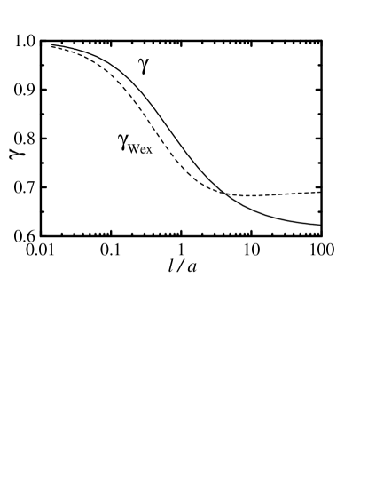
FIG. 2.: The dependence of factor $\gamma$ in Eq. (88) on the ratio $\ell/a$. Also shown is the variational calculation of $\gamma_{\mathrm{Wex}}$ from Ref. 4.

Section II formulates the algebra and Sec. III explains the solution.

II Semiclassical transport theory in the orifice geometry

In order to find the current density ${\bf j}({\bf r})$ through orifice, in the semiclassical approach, we have to solve simultaneously the stationary Boltzmann equation in the presence of an electric field and the Poisson equation for the electric potential

$$\dot{\bf r}\cdot\frac{\partial F({\bf k,r})}{\partial{\bf r}}-\frac{e\nabla\Phi({\bf r})}{\hbar}\cdot\frac{\partial F({\bf k,r})}{\partial{\bf k}} = -\frac{F({\bf k,r})-f_{\mathrm{L}E}({\bf k,r})}{\tau},$$ (5)

$$\nabla^{2}\Phi({\bf r}) = -\frac{e\delta n({\bf r})}{\epsilon},$$ (6)

$$\delta n({\bf r}) = \frac{1}{\Omega}\sum_{\bf k}(F({\bf k,r})-f({\epsilon_{k}})),$$ (7)

$$0 = \frac{1}{\Omega}\sum_{\bf k}(F({\bf k,r})-f_{\mathrm{L}E}({\bf k,r})),$$ (8)

$${\bf j({\bf r})} = \frac{e}{\Omega}\sum_{\bf k}{\bf v_{k}}F({\bf k,r}).$$ (9)

Here $F({\bf k,r})$ is the distribution function, $f({\epsilon_{k}})$ is the equilibrium Fermi-Dirac function, $\Phi({\bf r})$ is electric potential, $\Omega$ is the volume of the sample and $f_{\mathrm{L}E}({\bf k,r})$ is a Fermi-Dirac function with spatially varying chemical potential $\mu({\bf r})$ which has the same local charge density as $F({\bf k,r})$. In general, we have to deal with the local deviation $\delta n({\bf r})$ of electron density from its equilibrium value self-consistently. The collision integral is written in the standard relaxation time approximation with scattering time $\tau=l/v_{F}$. This system of equations should be supplemented with boundary conditions on the left electrode (LE) at $z=-\infty$, right electrode (RE) at $z=\infty$, and on the impermeable diaphragm $(D)$ at $z=0$:

$$\Phi({\bf r}_{\mathrm{L}E}) = V,$$ (11)

$$\Phi({\bf r}_{\mathrm{R}E}) = -V,$$ (12)

$$j_{z}({\bf r}_{D}) = 0,$$ (13)

where $z$-axis is taken to be perpendicular to the orifice. In linear approximation we can express the distribution function $F({\bf k,r})$ and local equilibrium distribution function $f_{\mathrm{L}E}({\bf k,r})$ using $\delta\mu({\bf r})$ (local change of the chemical potential) and $\Psi({\bf k,r})$ (deviation function, i.e. energy shift of the altered distribution)

$$f_{\mathrm{LE}}({\bf k,r}) = f(\epsilon_{k}-\delta\mu({\bf r}))\approx f(\epsilon_{k})-\frac{\partial f(\epsilon_{k})}{\partial\epsilon_{k}}\delta\mu({\bf r}),$$ (14)

$$F({\bf k,r}) = f(\epsilon_{k}-\Psi({\bf k,r}))\approx f(\epsilon_{k})-\frac{\partial f(\epsilon_{k})}{\partial\epsilon_{k}}\Psi({\bf k,r}).$$ (15)

These equations imply that $\delta\mu({\bf r})$ is identical to the angular average of $\Psi({\bf k,r})$

$$\delta n({\bf r})=\frac{1}{\Omega}\sum_{\bf k}-\frac{\partial f(\epsilon_{k})}{\partial\epsilon_{k}}\Psi({{\bf k,r}})=N(0)\langle\Psi({\bf r})\rangle=N(0)\delta\mu({\bf r}),$$ (16)

where $N(0)$ is the density of states at the Fermi energy $\epsilon_{F}$. In the case of a spherical Fermi surface,

$$\langle\Psi({\bf r})\rangle=\frac{1}{4\pi}\int d\Omega_{k}\Psi({\bf k,r}).$$ (17)

Following Wexler [4], we introduce a function $u({\bf k,r})$ by writing $\Psi({\bf k,r})$ as

$$\Psi({\bf k,r})=eVu({\bf k,r})-e\Phi({\bf r}).$$ (18)

Thereby, the linearized Boltzmann equation (5) becomes an integro-differential equation for the function $u({\bf k,r})$

$$\tau{\bf v_{k}}\cdot\frac{\partial u({\bf k,r})}{\partial{\bf r}}=\langle u({\bf r})\rangle-u({\bf k,r}).$$ (19)

To solve this equation we need to know only boundary conditions satisfied by $u({\bf k,r})$ and then we can use this solution to find the potential $\Phi({\bf r})$. Thus the calculation of the conductance from $u({\bf k,r})$ is decoupled from the Poisson equation. This is an intrinsic property of linear response theory [10]. The boundary conditions for (19) are:

$$\langle u({\bf r}_{\mathrm{L}E})\rangle = 1,$$ (21)

$$\langle u({\bf r}_{\mathrm{R}E})\rangle = -1.$$ (22)

They follow from the boundary conditions (11)-(12) for the potential $\Phi({\bf r})$ and the fact that far away from the orifice we can expect local charge neutrality entailing

$$\langle u({\bf r})\rangle=\frac{\Phi({\bf r})}{V}.$$ (23)

The driving force is explicitly absent from (19), but it enters the problem through these boundary conditions. Since Eq. (19) is invariant under the reflection in the plane of diaphragm

$$({\bf k,r}) \rightarrow ({\bf k}^{R},{\bf r}^{R}),$$ (25)

$${\bf r}^{R} = (x,y,-z),$$ (26)

$${\bf k}^{R} = (k_{x},k_{y},-k_{z}),$$ (27)

the boundary conditions imply that $u({\bf k,r})$ has reflection antisymmetry

$$u({\bf k,r})=-u({\bf k}^{R},{\bf r}^{R}).$$ (28)

Wexler’s solution [4] to the equation (19) relied on the equivalence between the problem of orifice resistance and spreading resistance of a disk electrode in the place of orifice. Technically this is achieved by switching from the equation for function $u({\bf k,r})$ to the equation for function

$$w({\bf k,r})=1+\mathrm{sgn}\,(z)u({\bf k,r}).$$ (29)

The beauty of this transformation is that new function allows us to replace the discontinuous behavior of $u({\bf k,r})$ on the diaphragm (which is the mathematical formulation of specular scattering)

$$u({\bf k,r}_{D}-{\bf v_{k}}dt)=u({\bf k}^{R},{\bf r}_{D}-{\bf v_{k}}dt)=-u({\bf k},{\bf r}_{D}+{\bf v_{k}}dt)$$ (30)

with continuous behavior of $w({\bf k,r})$ over the diaphragm, discontinuous behavior over the orifice and simpler boundary conditions on the electrodes

$$\langle w({\bf r}_{\mathrm{L}E})\rangle=\langle w({\bf r}_{\mathrm{R}E})\rangle=0.$$ (31)

The Boltzmann equation (19) now becomes

$$\mathchoice{{\hbox{\boldmath$\displaystyle\ell$}}}{{\hbox{\boldmath$\textstyle\ell$}}}{{\hbox{\boldmath$\scriptstyle\ell$}}}{{\hbox{\boldmath$\scriptscriptstyle\ell$}}}_{\bf k}\cdot\frac{\partial w({\bf k,r})}{\partial{\bf r}}+w({\bf k,r})-\langle w({\bf r})\rangle=s({\bf k,r})\delta(z)\theta(a-r),$$ (32)

where we have introduced the function

$$s({\bf k,r})=2\ell_{\mathrm{k}z}u({\bf k,r})$$ (33)

which is confined to the orifice region. It can be related to $w({\bf k,r})$ at the orifice in the following way:

$$s({\bf k,r}_{0})=2|\ell_{\mathrm{k}z}|(1-w({\bf k,r}_{0}-{\bf v_{k}}dt)).$$ (34)

It plays the role of a “source of particles” in Eq. (32). The notation ${\bf r}_{0}$ refers to a vector lying on the orifice, that is ${\bf r}_{0}=(x,y,0)$ with $x^{2}+y^{2}\leq a^{2}$. The discontinuity of $w({\bf k,r})$ on the orifice is handled by replacing it by the disk electrode which spreads particles into a scattering medium.

The Green’s function for Eq. (32) is the inverse Boltzmann operator (including boundary conditions)

$$\left(\mathchoice{{\hbox{\boldmath$\displaystyle\ell$}}}{{\hbox{\boldmath$\textstyle\ell$}}}{{\hbox{\boldmath$\scriptstyle\ell$}}}{{\hbox{\boldmath$\scriptscriptstyle\ell$}}}_{\bf k}\cdot\frac{\partial}{\partial{\bf r}}+1-\hat{A}\right)G_{B}({\bf k,r;k^{\prime},r^{\prime}})=\delta(\Omega_{k}-\Omega_{k^{\prime}})\delta({\bf r-r^{\prime}}),$$ (35)

and $\hat{A}$ is the angular average operator

$$\hat{A}f({\bf k})=\frac{1}{4\pi}\int d\Omega_{k}\,f({\bf k})=\langle f\rangle.$$ (36)

The Green’s function for the Boltzmann equation allows us to express $w({\bf k,r}_{0}-{\bf v_{k}}dt)$ in the form of a four-dimensional integral equation over the surface of the orifice

$$w({\bf k,r}_{0}-{\bf v_{k}}dt)=\int d\Omega_{k^{\prime}}\,d{\bf r^{\prime}}_{0}\,G_{B}({\bf k,r}_{0}-{\bf v_{k}}dt;{\bf k^{\prime},r^{\prime}}_{0}+{\bf v_{k^{\prime}}}dt)s({\bf k^{\prime},r^{\prime}}_{0}).$$ (37)

The function $w({\bf k,r})$ is discontinuous over the orifice, so we formulate the equation for this function at points infinitesimally close $(dt\rightarrow+0)$ to the orifice. We find the following explicit expression for the Green’s function

$$G_{B}({\bf k,r;k^{\prime},r^{\prime}})=\frac{1}{\Omega}\sum_{\bf q}\frac{e^{i{\bf q\cdot(r-r^{\prime})}}}{1+i{\bf q\cdot}\mathchoice{{\hbox{\boldmath$\displaystyle\ell$}}}{{\hbox{\boldmath$\textstyle\ell$}}}{{\hbox{\boldmath$\scriptstyle\ell$}}}{{\hbox{\boldmath$\scriptscriptstyle\ell$}}}_{\bf k}}\left(\delta(\Omega_{k}-\Omega_{k^{\prime}})+\frac{q\ell(q\ell-\arctan q\ell)^{-1}}{4\pi(1+i{\bf q\cdot}\mathchoice{{\hbox{\boldmath$\displaystyle\ell$}}}{{\hbox{\boldmath$\textstyle\ell$}}}{{\hbox{\boldmath$\scriptstyle\ell$}}}{{\hbox{\boldmath$\scriptscriptstyle\ell$}}}_{\bf k^{\prime}})}\right).$$ (38)

Its form reflects the separable structure of Boltzmann operator, i.e. the sum of operators whose factors act in the space of functions of either $\bf r$ or $\bf k$. However it is nontrivial because the factors acting in $\bf k$-space do not commute and the Boltzmann operator is not normal—it does not have the complete set of eigenvectors and the standard procedure for constructing the Green’s function from the projectors on these states fails. The first term in (38) is singular and generates the discontinuity of $w({\bf k,r})$ over the orifice.

III The Conductance of the orifice

The conductance of the orifice is defined by

$$G=\frac{1}{R}=\frac{I}{2V}=\frac{\int{d{\bf r}_{0}\,j_{z}({\bf r}_{0})}}{2V},$$ (39)

where the $z$-component of the current at the surface of the orifice is

$$j_{z}({\bf r}_{0})=\frac{N(0)e^{2}V}{8\pi\tau}\int{d{\Omega_{k}}\,s({\bf k,r}_{0})}.$$ (40)

The Green’s function result (38) allows us to rewrite Eq. (37) in the following integral equation for the smooth function $s({\bf k,r}_{0})$ over the surface of the orifice

$$1=\frac{s({\bf k,r}_{0})}{2|\ell_{\mathrm{k}z}|}+\int d\Omega_{k^{\prime}}\,d{\bf r^{\prime}}_{0}\,G({\bf k,r}_{0};{\bf k^{\prime},r^{\prime}}_{0})s({\bf k^{\prime},r^{\prime}}_{0}),$$ (41)

where $G({\bf k,r}_{0};{\bf k^{\prime},r^{\prime}}_{0})$ is non-singular part of the Green’s function (38)

$$G({\bf k,r}_{0};{\bf k^{\prime},r^{\prime}}_{0})=\frac{1}{32\pi^{4}}\int d{\bf q}\,\frac{q\ell\,e^{i{\bf q\cdot(r}_{0}-{\bf r^{\prime}}_{0})}}{(1+i{\bf q\cdot}\mathchoice{{\hbox{\boldmath$\displaystyle\ell$}}}{{\hbox{\boldmath$\textstyle\ell$}}}{{\hbox{\boldmath$\scriptstyle\ell$}}}{{\hbox{\boldmath$\scriptscriptstyle\ell$}}}_{\bf k})(q\ell-\arctan q\ell)(1+i{\bf q\cdot}\mathchoice{{\hbox{\boldmath$\displaystyle\ell$}}}{{\hbox{\boldmath$\textstyle\ell$}}}{{\hbox{\boldmath$\scriptstyle\ell$}}}{{\hbox{\boldmath$\scriptscriptstyle\ell$}}}_{\bf k^{\prime}})}.$$ (42)

The distribution function $s({\bf k,r}_{0})$ has two ${\bf k}$-space variables, the polar and azimuthal angles $(\theta_{k},\phi_{k})$ of the vector ${\bf k}$ on the Fermi surface, and the radius $r_{0}$ and azimuthal angle $\phi_{0}$ of the point ${\bf r}_{0}$ on the orifice. Because of the cylindrical symmetry, $s({\bf k,r}_{0})$ does not depend separately on $\phi_{k}$, $\phi_{0}$, but only on their difference $\phi_{k}-\phi_{0}$. This allows the expansion

$$s({\bf k,r}_{0})=\sum_{LM}{s_{\mathrm{L}M}(r_{0})Y_{\mathrm{L}M}(\theta_{k},\phi_{k})e^{-iM\phi_{0}}},$$ (43)

and Eq. (41) can now be rewritten as

$$2\ell\cos\theta_{k} = \sum_{L^{\prime}M^{\prime}}s_{\mathrm{L}^{\prime}M^{\prime}}(r_{0})Y_{\mathrm{L}^{\prime}M^{\prime}}(\theta_{k},\phi_{k})e^{-iM^{\prime}\phi_{0}}\mathrm{sgn}\,(\cos\theta_{k})$$ (45)

$$+2\ell\int d{\Omega_{k^{\prime}}}\,d{\bf r^{\prime}}_{0}\,G({\bf k,r}_{0};{\bf k^{\prime},r^{\prime}}_{0})\cos\theta_{k}\sum_{L^{\prime}M^{\prime}}s_{\mathrm{L}^{\prime}M^{\prime}}(r^{\prime}_{0})Y_{\mathrm{L}^{\prime}M^{\prime}}(\theta_{k^{\prime}},\phi_{k^{\prime}})e^{-iM^{\prime}\phi^{\prime}_{0}}.$$

This four dimensional integral equation can be reduced to a system of coupled one dimensional Fredholm integral equations of the second kind after it is multiplied by $Y_{\mathrm{L}M}^{\ast}(\theta_{k},\phi_{k})e^{iM\phi_{0}}$ and integrated over $\theta_{k}$, $\phi_{k}$ and $\phi_{0}$. We also use the following identities

$$Y_{\mathrm{L}M}(\theta,\phi)\,\cos\theta = g_{1}Y_{\mathrm{L}+1,M}(\theta,\phi)+g_{2}Y_{\mathrm{L}-1,M}(\theta,\phi),$$ (47)

$$g_{1} = \sqrt{\frac{(L-M+1)(L+M+1)}{(2L+1)(2L+3)}},$$ (48)

$$g_{2} = \sqrt{\frac{(L-M)(L+M)}{(2L-1)(2L+1)}},$$ (49)

$$\frac{1}{4\pi}\int\frac{Y_{\mathrm{LM}}(\theta_{k},\phi_{k})}{1+i{\bf q\cdot}\mathchoice{{\hbox{\boldmath$\displaystyle\ell$}}}{{\hbox{\boldmath$\textstyle\ell$}}}{{\hbox{\boldmath$\scriptstyle\ell$}}}{{\hbox{\boldmath$\scriptscriptstyle\ell$}}}_{\bf k}}\,d\Omega_{k}=i^{L}f_{L}(q\ell)Y_{\mathrm{LM}}(\theta_{q},\phi_{q}),$$ (50)

and

$$\int_{0}^{2\pi}e^{i{\bf qr}_{0}}e^{-iM\phi_{0}}\,d\phi_{0}=\int_{0}^{2\pi}e^{iq_{\perp}r_{0}\cos(\phi_{0}-\phi_{q})}e^{-iM\phi_{0}}\,d\phi_{0}=2\pi i^{M}J_{M}(q_{\perp}r_{0})e^{-iM\phi_{q}},$$ (51)

where ${\bf q_{\perp}}$ is projection of ${\bf q=q_{z}+q_{\perp}}$ in the plane of orifice and $J_{M}(z)$ is the Bessel function of the first kind. For the function $f_{L}(q\ell)$ in (50) we get the following expression

$$f_{L}(q\ell)=(-1)^{L}\int_{0}^{\infty}e^{-x}j_{L}(q\ell x)\,dx=\frac{(-i)^{-L}}{iq\ell}Q_{L}(\frac{1}{iq\ell}),$$ (52)

where $j_{L}(x)$ is spherical Bessel function and $Q_{L}(x)$ is Legendre function of the second kind. Explicit formulae for $f_{L}(x)$ are

$$f_{0}(x) = \frac{\arctan x}{x},$$ (54)

$$f_{1}(x) = \frac{-x+\arctan x}{x^{2}},$$ (55)

$$f_{2}(x) = \frac{-3x+(x^{2}+3)\arctan x}{2x^{3}},$$ (56)

$$f_{3}(x) = \frac{-\frac{4}{3}x^{3}-5x+(5+3x^{2})\arctan x}{2x^{4}},$$ (57)

$$f_{4}(x) = \frac{-\frac{55}{3}x^{3}-35x+(35+30x^{2}+3x^{4})\arctan x}{8x^{5}}.$$ (58)

The final form of the integral equation for $s_{\mathrm{LM}}(r_{0})$ in the expansion of $s({\bf k,r}_{0})$ is

$$4\ell\sqrt{\frac{\pi}{3}}\delta_{L1}\delta_{M0}=\sum_{\mathrm{L^{\prime}M^{\prime}}}c_{\mathrm{LM,L^{\prime}M^{\prime}}}\delta_{\mathrm{M}M^{\prime}}s_{\mathrm{L^{\prime}M^{\prime}}}(r_{0})+4\sum_{L^{\prime}M^{\prime}}\int_{0}^{a}r^{\prime}_{0}\,dr^{\prime}_{0}\,K_{\mathrm{LM,L^{\prime}M^{\prime}}}(r_{0},r^{\prime}_{0})s_{\mathrm{L^{\prime}M^{\prime}}}(r^{\prime}_{0}),$$ (59)

where the kernel of equation is given by

$$K_{\mathrm{LM,L^{\prime}M^{\prime}}}(r_{0},r^{\prime}_{0}) = i^{M^{\prime}-M}(-1)^{M+M^{\prime}}\int_{0}^{\infty}q^{2}\,dq\int_{0}^{\pi}\sin\theta_{q}\,d\theta_{q}\,\frac{q\ell^{2}f_{L^{\prime}}(q\ell)Y_{\mathrm{L}^{\prime}M^{\prime}}(\theta_{q})}{q\ell-\arctan q\ell}J_{M}(qr_{0}\,\sin\theta_{q})J_{M^{\prime}}(qr^{\prime}_{0}\,\sin\theta_{q})$$ (61)

$$\times(i^{L^{\prime}+L+1}(-1)^{L+1}g_{1}f_{L+1}(q\ell)Y_{\mathrm{L}+1,M}(\theta_{q})+i^{L^{\prime}+L-1}(-1)^{L-1}g_{2}f_{L-1}(q\ell)Y_{\mathrm{L}-1,M}(\theta_{q})).$$

Kernel (61) does not depend on $\phi_{q}$ so that only $\theta$-part of spherical harmonic $Y_{\mathrm{L}M}(\theta_{q})$ (i.e. associated Legendre polynomial) is integrated. The kernel differs from zero only if $L+M$ has parity different from $L^{\prime}+M^{\prime}$. This follows from the fact that the kernel is the expectation value

$$K_{\mathrm{L}M,L^{\prime}M^{\prime}}(r_{0},r^{\prime}_{0}) = \langle LMM|2\ell\,\cos\theta\,G({\bf k,r}_{0};{\bf k^{\prime},r^{\prime}}_{0})|L^{\prime}M^{\prime}M^{\prime}\rangle,$$ (62)

$$|LMM\rangle = Y_{\mathrm{LM}}(\theta_{k},\phi_{k})e^{-iM\phi_{0}}$$ (63)

of an odd operator under inversion in the basis of functions $|LMM\rangle$. Their parity is given by

$$P|LMM\rangle=(-1)^{L+M}|LMM\rangle.$$ (64)

Exactly under this condition the kernel becomes a real quantity. This means that nonzero $s_{\mathrm{L}M}(r_{0})$ are real with the property

$$s_{\mathrm{L}M}(r_{0})=(-1)^{M}s_{\mathrm{L},-M}(r_{0}),$$ (65)

ensuring that $s({\bf k,r}_{0})$ is real. The conductance is determined by the $(L,M)=(0,0)$ function $s_{00}(r_{0})$. The non-zero $s_{\mathrm{LM}}(r_{0})$ coupled to it are selected by the condition that $L+M$ is even. This follows from $s({\bf k,r}_{0})$ being even under reflection in the plane of orifice. Under this operation, $\cos\theta_{k}\rightarrow-\cos\theta_{k}$, but $\phi_{k}$, $\phi_{0}$ are unchanged; this means that the expansion (43) contains only terms with $L+M$ even.

The first term on the right hand side in (45) is determined by the matrix element

$$c_{\mathrm{LM,L^{\prime}M^{\prime}}}=\int d\theta_{k}\,d\phi_{k}\,\sin\theta_{k}Y_{\mathrm{LM}}^{\ast}(\theta_{k},\phi_{k})Y_{\mathrm{L^{\prime}M^{\prime}}}(\theta_{k},\phi_{k})\,\mathrm{sgn}\,(\cos\theta_{k}),$$ (66)

which is expectation value of $\mathrm{sgn}\,(\cos\theta_{k})$ in the basis of spherical harmonics. It is different from zero if $M=M^{\prime}$ and $L-L^{\prime}$ is odd. The states must be of of different parity, as determined by $L$, because $\mathrm{sgn}\,(\cos\theta_{k})$ is odd under inversion.

The system of equations (59) can be solved for all possible ratios of $\ell/a$ by either discretizing variable $r_{0}$ or by expanding $s_{\mathrm{L}^{\prime}M^{\prime}}(r_{0})$ in terms of the polynomials in $r_{0}$

$$s_{\mathrm{LM}}(r_{0})=\sum_{n}a_{\mathrm{nLM}}p_{n}(r_{0}),$$ (67)

and performing integrations numerically. The polynomials $p_{n}(r_{0})=\sum_{i=0}^{n}c_{i}r^{i}$ are orthogonal with respect to the scalar product

$$\int_{0}^{a}r_{0}\,dr_{0}\,p_{n}(r_{0})p_{m}(r_{0})=\delta_{nm}.$$ (68)

The first three polynomials are

$$p_{0}(r_{0}) = \frac{\sqrt{2}}{a},$$ (70)

$$p_{1}(r_{0}) = \frac{6r_{0}-4}{a\sqrt{9a^{2}-16a+9}},$$ (71)

$$p_{2}(r_{0}) = \frac{10\sqrt{6}\left(r_{0}^{2}-\frac{6}{5}r_{0}+\frac{3}{10}\right)}{a\sqrt{100a^{4}-288a^{3}+306a^{2}-144a+27}}.$$ (72)

Each integral equation in the system (59) then becomes the matrix equation. Their introduction into inherent matrix structure of (59) gives the matrix equation for either $s_{\mathrm{L}M}(r_{0})$ at discretized $r_{0}$ or constants $a_{\mathrm{nLM}}$. Therefore, the constants $a_{\mathrm{nLM}}$ satisfy the following equation

$$4\ell a\sqrt{\frac{\pi}{6}}\delta_{L1}\delta_{M0}\delta_{n0}=\sum_{L^{\prime}}c_{\mathrm{LM,L^{\prime}M}}\,a_{\mathrm{nL^{\prime}M}}+4\sum_{n^{\prime}L^{\prime}M^{\prime}}K_{\mathrm{nLM}}^{\mathrm{n^{\prime}L^{\prime}M^{\prime}}}a_{\mathrm{n^{\prime}L^{\prime}M^{\prime}}},$$ (74)

$$K_{\mathrm{nLM}}^{\mathrm{n^{\prime}L^{\prime}M^{\prime}}} = i^{M^{\prime}-M}(-1)^{M+M^{\prime}}\int_{0}^{\infty}q^{2}\,dq\int_{0}^{\pi}\sin\theta_{q}\,d\theta_{q}\,\frac{q\ell^{2}f_{L^{\prime}}(q\ell)Y_{\mathrm{L}^{\prime}M^{\prime}}(\theta_{q})}{q\ell-\arctan q\ell}j^{n}_{M}(qa\,\sin\theta_{q})j^{n^{\prime}}_{M^{\prime}}(qa\,\sin\theta_{q})$$ (76)

$$\times(i^{L^{\prime}+L+1}(-1)^{L+1}g_{1}f_{L+1}(q\ell)Y_{\mathrm{L}+1,M}(\theta_{q})+i^{L^{\prime}+L-1}(-1)^{L-1}g_{2}f_{L-1}(q\ell)Y_{\mathrm{L}-1,M}(\theta_{q})),$$

$$j^{n}_{M}(qa\,\sin\theta_{q}) = \int_{0}^{a}r_{0}\,dr_{0}\,p_{n}(r_{0})J_{M}(qr_{0}\,\sin\theta_{q}),$$ (77)

which simplifies using the following result

$$j^{n}_{M}(qa\,\sin\theta_{q})=\sum_{i=0}^{n}c_{i}\frac{{a}^{2+M+i}(q\,\sin\theta_{q})^{M}{{}_{1}F_{2}}(1+\frac{M}{2}+\frac{i}{2};2+\frac{M}{2}+\frac{i}{2},1+M;-\frac{1}{4}(qa\,\sin\theta_{q})^{2})}{2^{1+M}\left(1+\frac{M}{2}+\frac{i}{2}\right)\Gamma(1+M)},$$ (78)

where ${}_{1}F_{2}(\alpha;\beta_{1},\beta_{2};z)$ is a hypergeometric function. The lowest order approximation for $s({\bf k,r}_{0})$ is obtained by truncating the polynomial expansion to zeroth order (i.e. constant—which is the space dependence of Sharvin limit) and expansion in spherical harmonics to $L=0$. Then the conductance is determined only by the constant $a_{000}$ following trivially from (III)

$$G_{\mathrm{l}o}=\frac{N(0)\ell e^{2}a^{2}\pi}{\tau(3+K_{010}^{000})},$$ (79)

where the lowest order part of the kernel $K_{010}^{000}$ depends on $\ell/a$,

$$K_{010}^{000}=\frac{4\ell}{\pi}\int_{0}^{\infty}dq\,\int_{0}^{\pi}d\theta_{q}\,\frac{\arctan q\ell}{q\ell-\arctan q\ell}\left(\frac{-3q\ell+(q^{2}\ell^{2}+3)\arctan q\ell}{2q^{3}\ell^{3}}(1-3\cos^{2}\theta_{q})+\frac{\arctan q\ell}{q\ell}\right)\frac{(J_{1}(qa\,\sin\theta_{q}))^{2}}{\sin\theta_{q}}.$$ (80)

Further corrections are obtained by solving the matrix equation (III) where the infinite matrix is approximated by its finite block. The matrix elements $K_{\mathrm{nLM}}^{\mathrm{n^{\prime}L^{\prime}M^{\prime}}}$ (76) are tedious to compute, but the conductance converges rapidly for large $n$ and $L$. On the other hand, the matrix elements $c_{\mathrm{LM,L^{\prime}M^{\prime}}}$ (66) are easy to compute but the conductance converges slowly in the ballistic limit which is determined by this matrix elements. We keep the low order matrix elements $K_{\mathrm{nLM}}^{\mathrm{n^{\prime}L^{\prime}M^{\prime}}}$ but go to high order in $c_{\mathrm{LM,L^{\prime}M^{\prime}}}$. In practice we find that for $c$-matrix $L_{\mathrm{m}ax}=12$ is sufficient, whereas for $K$-matrix the approximation $L_{\mathrm{m}ax}=2$, $n_{\mathrm{m}ax}=2$ gives convergence to $1\%$. The conductance as a function of $\ell/a$ is shown on Fig. 3. It is normalized to the Sharvin conductance, i.e. conductance in the limit $\ell\gg a$, for which

$$G({\bf k,r;k^{\prime},r^{\prime}}) \rightarrow 0,$$ (81)

$$s({\bf k,r}) = 2|\ell_{\mathrm{k}z}|.$$ (82)

In the opposite (Maxwell) limit, when $\ell\ll a$, we have

$$\frac{q\ell}{q\ell-\arctan q\ell} = \frac{3}{(q\ell)^{2}}+9/5+o((q\ell)^{2}),$$ (84)

$$G({\bf k,r;k^{\prime},r^{\prime}}) \rightarrow \frac{3}{32\pi^{4}}\int d{\bf q}\,\frac{e^{i{\bf q\cdot(r-r^{\prime})}}}{(q\ell)^{2}}=\frac{3}{16\pi^{2}\ell^{2}|{\bf r-r^{\prime}}|},$$ (85)

which is the standard Green’s function for the Poisson equation. The dependence of the full Green’s function (38) on ${\bf k}$ vector is reflection of non-locality. The conductance in the transition region from Maxwell to Sharvin limit can be compared with the naive interpolation formula which approximates resistance of orifice by the sum of Sharvin and Maxwell resistances

$$\frac{1}{G_{I}}=R_{I}=R_{S}\left(1+\frac{3\pi}{8}\frac{a}{\ell}\right).$$ (86)

Somewhat unexpectedly, naive interpolation formula $G_{I}$ deviates from our result for $G$ at most $11\%$ when $\ell/a\rightarrow 1$ as shown on Fig. 3. We can also cast our lowest order approximation for the conductance (79) in an analogous form as (86)

$$\frac{1}{G_{\mathrm{l}o}}=R_{S}\left(\frac{3}{4}+\frac{32}{3\pi^{2}}\gamma\frac{3\pi}{8}\frac{a}{\ell}\right).$$ (87)

The numerical coefficients in Eq. (87) are not accurate in this simplest approximation. Replacement of $3/4$ by $1$ and $32/(3\pi^{2})$ by $1$ yields correct limiting values of $G$ and leads to a plausible interpolation formula. It differs from Eq. (86) by the introduction of a factor $\gamma$ which multiplies the Maxwell resistance

$$\frac{1}{G_{0}}=R_{S}\left(1+\gamma\frac{3\pi}{8}\frac{a}{\ell}\right),$$ (88)

$$\gamma=\frac{\pi\ell}{16a}K_{010}^{000}.$$ (89)

This formula is compared to $G$ and $G_{I}$ on Fig. 3. It differs from our most accurate calculation of $G$ by less then $1\%$. Therefore, for all practical purposes it can be used as an exact expression for the conductance in this geometry, and it is the main outcome of our work. The factor $\gamma$ is of order one and depends on the ratio $\ell/a$ as shown on Fig. 2. We also plot on Fig. 2 Wexler’s [4] previous variational calculation, $\gamma_{\mathrm{Wex}}$.

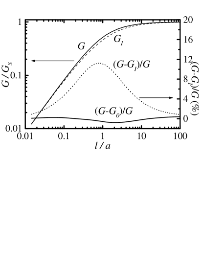
FIG. 3.: The conductance $G$ ($L=2$, $n=2$), normalized by the Sharvin conductance $G_{S}$ (2), plotted against the ratio $\ell/a$. It is compared to the naive interpolation formula $G_{I}$ (86), and the plausible interpolation formula $G_{0}$ (88).

In conclusion, we have calculated the conductance of the orifice in all transport regimes, from the diffusive to the ballistic. The altered version (88) of the simplest approximate solution of our theory (79) is already reasonably accurate. It shows the microscopic theory correction to the naive interpolation formula (sum of Maxwell and Sharvin resistances) which is within $11\%$ different from the exact answer. Further corrections converge rapidly to an exact result. This analysis is of interest in any situation where the geometry of the sample can introduce additional resistances, like for example in transport in granular materials [11].

This work was supported in part by the NSF grant no. DMR 9725037.

REFERENCES

- [1] J. C. Maxwell, A Treatise on Electricity and Magnetism (Dover Press, New York, 1891).
- [2] Yu. V. Sharvin, Zh. Eksp. Teor. Fiz. 48, 984 (1965) [Sov. Phys. JETP 21, 655 (1965)].
- [3] R. Landauer, IBM J. Res. Dev. 1, 223 (1957); Phil. Mag. 21, 863 (1970); M. Büttiker, Phys. Rev. Lett. 57, 1761 (1986).
- [4] G. Wexler, Proc. Phys. Soc. London 89, 927 (1966).
- [5] I. O. Kulik, A. N. Omelyanchuk, R. I. Shekter, Fiz. Nizk. Temp. 3, 1543 (1977) [Sov. J. Low Temp. Phys. 3, 740 (1977)].
- [6] I. F. Itskovitch and R. Shekter, Fiz. Nizk. Temp. 11, 373 (1985) [Sov. J. Low Temp. Phys. 11 202 (1985)].
- [7] N. J. M. Jensen, A. P. van Gelder, A. M. Duif, P. Wyder, and N. d’Ambrumenil, Helv. Phys. Acta 56, 209 (1983).
- [8] B. J. van Wees, H. van Houten, C. W. J. Beenaker, J. G. Williamson, L. P. Kouwenhoven, D. van der Marel, and C. T. Foxon, Phys. Rev. Lett. 60, 848 (1988).
- [9] D. A. Wharam, T. J. Thornton, R. Newbury, M. Pepper, H. Ahmed, J. E. F. Frost, D. G. Hasko, D. C. Peacock, D. A. Ritchie, and G. A. C. Jones, J. Phys. C 21, L209 (1988).
- [10] C. W. J. Beenaker and H. van Houten, in Solid State Physics: Advances in Research and Applications, edited by H. Ehrenreich and D. Turnbull (Academic Press, New York, 1991), v. 44, p. 1.
- [11] S. B. Arnason, S. P. Herschfield, and A. F. Hebard, Phys. Rev. Lett. 81, 3936 (1998).