A Stochastic Liouvillian Algorithm to Simulate Dissipative Quantum Dynamics
With Arbitrary Precision

Abstract

An exact and efficient new method to simulate dynamics in dissipative quantum systems is presented. A stochastic Liouville equation, deduced from Feynman and Vernon’s path-integral expression of the reduced density matrix, is used to describe the exact dynamics at any dissipative strength and for arbitrarily low temperatures. The utility of the method is demonstrated by applications to a damped harmonic oscillator and a double-well system immersed in an Ohmic bath at low temperatures.

Relaxation dynamics and fluctuations of a quantum system in contact with a thermal bath are improtant for many different areas of chemistry and physics, such as reaction-rate theory[1, 2], ultrafast phenomena in chemistry and biochemistry[3], tunneling at defects in solids[4] and quantum optics. While some limiting cases permit Markovian or weak-coupling approximations to the dissipation effects, the majority of others do not. Problems involving coherence[5] are prime examples in which the Markovian approximation fails.

The exact treatment of dissipative dynamics presented here is based on the path integral influence functional formalism[6], developed by Feynman and Vernon for interacting systems and extensively used in dissipative quantum mechanics[7, 8]. The main difficulty in evaluating the complex-valued path integral involved is that the integrand is not a local functional of the paths. Except for the case where the memory effects decay on a short time scale[9], deterministic integration methods fail, making it prohibitively expensive in both computation time and memory requirements. To date, the only exact numerical approach to dissipative quantum dynamics with arbitrary memory time has been the dynamical quantum Monte Carlo (QMC) method. This method, however, is severely limited by the sign problem, i.e. the signal-to-noise ratio of the numerical result tends to zero exponentially with the time scale of the problem.

In this Letter, we deal with the problem with non-local influence functionals arising from arbitrary long bath memory. We recover fully time-local dynamics for the ubiquitous case of Ohmic dissipation by applying a simple Hubbard-Stratonovich transformation. The time-local path integral can then easily be solved by propagating an equation of motion for the reduced density matrix. The auxiliary quantity introduced by the transform appears in the dynamics as an additional classical time-varying force. The functional integration over the auxiliary quantity can be performed stochastically by interpreting it as a noise force. This yields a new and elegantly simple algorithm: Generate an ensemble of Gaussian noise trajectories with the appropriate spectrum, propagate the system for each noise trajectory, and average over the ensemble. In stark contrast to QMC methods, we find a statistical error that is virtually independent of time.

At a microscopic level, dissipation is caused by the interaction of a non-thermal system with a vast number of environmental modes at or close to thermal equilibrium. Although cumulative effects of these modes interacting with the system under study can have a drastic effect on its dynamics, the coupling to each individual mode is usually weak. This justifies the paradigmatic model employed by Caldeira and Leggett[10] to describe dissipative quantum systems – a particle in an arbitrary potential interacting linearly with a vast number of harmonic excitations,

$$H={p^{2}\over 2m}+V(q)+\sum_{\nu}{p_{\nu}^{2}\over 2m_{\nu}}+{m_{\nu}\omega_{\nu}^{2}\over 2}\left(x_{\nu}-{c_{\nu}\over m_{\nu}\omega_{\nu}^{2}}q\right)^{2}.$$ (1)

The effect of the environmental modes is fully characterized by their spectral density $J(\omega)={\pi\over 2}\sum_{\nu}{c_{\nu}^{2}\over m_{\nu}\omega_{\nu}}\delta(\omega-\omega_{\nu})$, which takes on the form $J(\omega)=\eta\omega$ in the Ohmic case, $\eta$ being the classical friction constant.

The time-dependent reduced density matrix is then given by a double path integral

$$\rho(q_{\rm f},q^{\prime}_{\rm f};t)=\int_{q_{\rm i}}^{q_{\rm f}}\!\!\!{\cal D}[q]\int_{q_{\rm i}}^{q^{\prime}_{\rm f}}\!\!\!{\cal D}[q^{\prime}]e^{{i\over\hbar}(S_{0}[q]-S_{0}[q^{\prime}])}F[q,q^{\prime}].$$ (2)

Here $S_{0}[q]$ is the action of the undamped quantum system, and its interactions with the environment are incorporated into a complex-valued influence functional $F[q,q^{\prime}]=\exp(-\Phi^{\prime}/\hbar-i\Phi^{\prime\prime}/\hbar)$ with

$$\Phi^{\prime}[q,q^{\prime}] = \int_{t_{0}}^{t}\!\!\!dt^{\prime}\int_{t_{0}}^{t^{\prime}}\!\!\!dt^{\prime\prime}(q(t^{\prime})-q^{\prime}(t^{\prime}))$$ (4)

$$\times L^{\prime}(t^{\prime}-t^{\prime\prime})(q(t^{\prime\prime})-q^{\prime}(t^{\prime\prime})),$$

$$\Phi^{\prime\prime}[q,q^{\prime}] = {1\over 2}\eta\int_{t_{0}}^{t}\!\!\!dt^{\prime}(q(t^{\prime})-q^{\prime}(t^{\prime}))$$ (6)

$$\times(\dot{q}(t^{\prime})+\dot{q}^{\prime}(t^{\prime})).$$

$L^{\prime}(t)$ is the real part of the autocorrelation function of the collective bath coordinate $\sum_{\nu}c_{\nu}x_{\nu}$, averaged over an ensemble of free oscillators.

This influence functional describes a ‘factorized’ initial preparation, i.e. with the particle constrained to an initial position $q_{i}$ for times $t<t_{0}$ [11] with the environment fully relaxed. Equilibrium correlation functions may be calculated by pushing the preparation back to a sufficiently large negative time $t_{0}<0$ [8] and inserting measurement operators at times $0$ and $t$.

In the following we outline the numerical solution of these equations using a novel technique we call the SLED (Stochastic Liouville Equation for Dissipation) method. SLED is based on the same principles as another method we recently introduced – the CSQD (Chromostochastic Quantum Dynamics) method[12]. Whereas CSQD was developed to treat discrete systems, SLED solves extended systems using a stochastic Liouvillian formalism.

The primary obstacle in trying to translate eqs. (2) – (6) into a recursion relation or an equation of motion for $\rho$ lies in the interaction kernel $L^{\prime}(t)$. Its range is often large, becoming divergent for $T\to 0$. This problem of retarded self-interactions mediated by $L^{\prime}(t)$ can be solved, albeit at the cost of introducing an additional path variable. The exponential of the non-local action $\Phi^{\prime}[q,q^{\prime}]$ can be decomposed into time-local phase factors,

$$\exp(-\Phi^{\prime}[q,q^{\prime}])=$$ (7)

$$\int{\cal D}[\xi]\,W[\xi]\exp\left\{-i\int_{t_{0}}^{t}\!\!\!dt^{\prime}\xi(t^{\prime})(q(t^{\prime})-q^{\prime}(t^{\prime}))\right\}.$$ (8)

The distribution function $W[\xi]$ is real and Gaussian, with $\langle\xi(t)\xi(t^{\prime})\rangle_{W}=L^{\prime}(t-t^{\prime})$, and normalizable through the condition $\Phi^{\prime}[q,q]\equiv 0$. Formally, this decomposition is just a Hubbard-Stratonovich transformation in a function space over the interval $[t_{0},t]$. Equation (7) is also equivalent to the construction of an influence functional for a classical colored noise source[6], and as such, we will interpret the function $\xi(t)$ as a noise trajectory and the measure ${\cal D}[\xi]W[\xi]$ as the probability measure of an ensemble of noise trajectories. For each noise trajectory, the reduced density matrix is then propagated deterministically according to the equation of motion

$$i\hbar\dot{\rho}={\cal L}_{0}\rho+{\cal L}_{\eta}\rho+\xi[q,\rho]$$ (9)

where ${\cal L}_{0}$ is the Liouvillian of the undamped system, and the friction term $\Phi^{\prime\prime}$ gives rise to an additional operator in the Liouvillian

$${\cal L}_{\eta}=-{\eta\over 2m}[q,\{p,\cdot\}].$$ (10)

The spectrum of the noise is determined by the spectral density and the temperature. In the Ohmic case, it is given by $S(\omega)=\eta\omega\coth(\hbar\beta\omega/2)$ up to an arbitrary but necessary cutoff frequency $\omega_{c}$. For computational purposes, it is advantageous to split off a ‘classical’ white noise part $S_{\rm cl}(\omega)=2\eta/\hbar\beta$ from this spectrum because it can be treated by a damping term

$${\cal L}_{d}=-i{\eta\over\hbar\beta}[q,[q,\cdot]]$$ (11)

that can be incorporated into the deterministic equation of motion in the Liouvillian rather than explicitly in the numerically generated noise field[13]. The full equation of motion then reads

$$i\hbar\dot{\rho}={\cal L}_{0}\rho+{\cal L}_{\eta}\rho+{\cal L}_{d}\rho+\tilde{\xi}[q,\rho]$$ (12)

where the noise spectrum of $\tilde{\xi}$ is $\tilde{S}(\omega)=S(\omega)-S_{\rm cl}(\omega)$. It has been shown previously [13] that using eq. (12) without the noise force $\tilde{\xi}$ is a limiting case that becomes exact only if $S(\omega)=S_{\rm cl}(\omega)$, i.e., for very high temperatures $kT\gg\hbar\omega_{c}$. Comparing the exact dynamics expressed in eq. (12) to this limiting case, we find a remarkable interpretation of our formalism: When a linear environment is treated classically, one generally incurs an error due to the missing quantum fluctuations. But by explicitly substituting an external noise force for the quantum fluctuations one actually regains the exact quantum dynamics at any temperature!

In the following we give examples, solving eq. (12) in the position representation using the split-propagator technique. The alternating direction implicit method is used for the operator ${\cal L}_{0}+\xi[q,\cdot]$ and an explicit method for the remaining term ${\cal L}_{\eta}+{\cal L}_{d}$. This choice is appropriate as it preserves the traceof $\rho$.

Our first test consists in the computation of the equilibrium correlation function $S(t)={1\over 2}\langle q(t)q(0)+q(0)q(t)\rangle$ of the damped harmonic oscillator, shown in Fig. 1, and its response function $\chi(t)={i\over\hbar}\langle[q(t),q(0)]\rangle$. At relatively high temperature, $kT=2\hbar\omega_{0}$, this calculation converges with only a handful trajectories and reproduces an almost classical result, as expected in this temperature regime. The initial value $S(0)$ corresponds exactly to the thermal expectation value $\langle q^{2}\rangle=kT/m\omega_{0}^{2}$. At low temperature, $kT=0.2\hbar\omega_{0}$, the fluctuation amplitude is no longer temperature-dependent, but is instead indicative of zero-point fluctuations. (Note that the initial amplitude for the damped oscillator is slightly reduced from the undamped value $\langle q^{2}\rangle=\hbar/2m\omega_{0}$[14]). In the same test, the susceptibility $\chi(t)$ of the quantum harmonic oscillator is determined. We find excellent agreement with the known analytic result $\chi(t)\equiv\chi_{\rm cl}(t)$. The high-temperature calculation completes within minutes, while the low-temperature calculation takes about $10^{3}$ trajectories for a very small absolute error $<0.007$, or 40 CPU hours on a midrange IBM Risc processor using a preliminary, non-optimized code.

For a more elaborate example, we use the quartic double-well potential $V(q)=q^{4}/4-q^{2}$, where natural units for time, mass, and energy are implied. In the undamped case, this system shows complex dynamics including both tunneling and vibrational oscillations. Fig. 2 shows the equilibrium dynamics of this system for different values of friction and temperature. For high friction, $\eta=0.5$, the system shows a monotonous decay, characteristic of incoherent relaxation (solid line). When the friction is lowered to $\eta=0.05$, a qualitative change to complex, anharmonic oscillatory dynamics is observed (dotted line). For the same friction, lowering the temperature leads to another qualitative change in the dynamics, resulting in damped oscillations with two manifestly distinct frequency scales (dashed line). The low-frequency component represents coherent tunneling, with a frequency related to the splitting between the two lowest energy eigenstates of the double well, and the high-frequency part derives from higher excited states.

In conclusion, we have developed a novel algorithm for the dynamics of extended dissipative quantum systems, which is highly efficient. It is also shown to be accurate on first principles and by explicit numerical tests. We have presented simulation data both for the damped harmonic oscillator and the dissipative double-well system which show the practical feasibility and power of this method. Empirically, we find that the statistical error of our results is extremely small, asymptotically approaching a constant value for long times. This implies a CPU requirement that scales linearly with the system time $t$, compared to the exponential rise for conventional quantum Monte Carlo methods. The SLED algorithm is also easily implemented on parallel computers. The system propagation for different noise realizations can be performed in parallel without any dependencies beyond the accumulation of final results.

We are currently extending the SLED method to study dynamics on electronically coupled energy surfaces in condensed-matter problems. The problem of greatest interest is the dynamics of electron transfer reactions in the inverted region. To model a bath with an arbitrary cutoff frequency, the SLED method has to be extended to treat systems with two electronic states coupled to a solvent mode which is in turn coupled to an Ohmic bath[15].

This research has been supported by the National Science Foundation under grant CHE-9528121. CHM is a NSF Young Investigator (CHE-9257094), a Camille and Henry Dreyfus Foundation Camille Teacher-Scholar and a Alfred P. Sloan Foundation Fellow. Computational resources have been provided by the IBM Corporation under the SUR Program at USC.

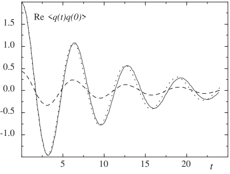
FIG. 1.: Equilibrium Fluctuations of the damped harmonic oscillator at $T=2$ (solid line) and $T=0.2$ (long dash) with $\hbar=k=m=1$, $\omega_{0}=1$, $\eta=0.2$. Short dashes indicate the analytic high-temparature solution[14] for $T=2$.

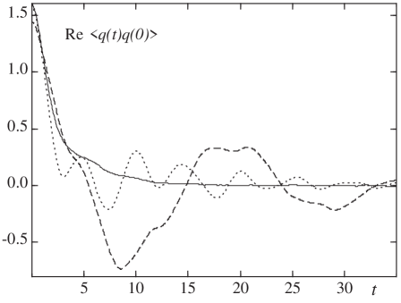
FIG. 2.: Equilibrium fluctuations of a dissipative double-well system for different friction constants. Solid line – dynamics showing incoherent decay for $\eta=0.5$, $T=1$. Dotted line – dynamics showing predominantly anharmonic vibronic oscillations for $\eta=0.05$, $T=1$. Dashed line – dynamics showing predominantly tunneling oscillations for $\eta=0.05$, $T=0.5$.

REFERENCES

- [1] P. Hänggi, P. Talkner and M. Borkovec, Rev. Mod. Phys. 62, 251 (1990).
- [2] D. Chandler, in: Liquids: Freezing and the Glass Transition, Les Houcshe 51, Part 1, D. Levesque, J.P. Hansen and J. Zinn-Justin, Eds., (Elsevier Science, North Holland, 1991).
- [3] R.A. Marcus and N. Sutin, Biochim. Biophys. Acta. 811, 265 (1985).
- [4] H. Wipf, D. Steinbinder, K. Neumaier, P. Gutsmiedl, A. Magerl, and A.J. Dianoux, Europhys. Lett. 4, 1379 (1987).
- [5] S. Chakravarty and A.J. Leggett, Phys. Rev. Lett. 52, 5 (1984).
- [6] R.P. Feynman and F.L. Vernon, Ann. Phys. (N.Y.) 24, 118 (1963).
- [7] A.J. Leggett, S. Chakravarty, A.T. Dorsey, M.P.A. Fisher, A. Garg and W. Zwerger, Rev. Mod. Phys. 59, 1 (1987), ibid., 67, 725 (1995).
- [8] U. Weiss, Quantum Dissipative Systems (World Scientific, Singapore, 1993).
- [9] D. Makarov and N. Makri, Chem. Phys. Lett. 221, 482 (1994).
- [10] A.O. Caldeira and A.J. Leggett, Phys. Rev. Lett. 46, 211 (1981).
- [11] The reduced density matrix at need not be localized at . The thermal density matrix of the undamped system is often a more convenient choice for the initial condition.
- [12] J.T. Stockburger and C.H. Mak, Phys. Rev. Lett. 80, 2657 (1998).
- [13] A.O. Caldeira and A.J. Leggett, Physica 121A, 587 (1983).
- [14] See, e.g., chapter 8 of Ref. [8].
- [15] A. Garg, J.N. Onuchic, and V. Ambegaokar, J. Chem. Phys. 83 4491 (1985).