Critical behavior of the planar magnet model in three dimensions

Abstract

We study the critical behavior of the three-dimensional planar magnet model in which each spin is considered to have three components of which only the $x$ and $y$ components are coupled. We use a hybrid Monte Carlo algorithm in which a single-cluster update is combined with the over-relaxation and Metropolis spin re-orientation algorithm. Periodic boundary conditions were applied in all directions. We have calculated the fourth-order cumulant in finite size lattices using the single-histogram re-weighting method. Using finite-size scaling theory, we obtained the critical temperature which is very different from that of the usual $XY$ model. At the critical temperature, we calculated the susceptibility and the magnetization on lattices of size up to $42^{3}$. Using finite-size scaling theory we accurately determine the critical exponents of the model and find that $\nu$=0.670(7), $\gamma/\nu$=1.9696(37), and $\beta/\nu$=0.515(2). Thus, we conclude that the model belongs to the same universality class with the $XY$ model, as expected.

I Introduction

Our understanding of critical phenomena has been significantly advanced with the development of the renormalization-group (RG) theory[1]. The RG theory predicts relationships between groups of exponents and that there is a universal behavior. In a second order phase transition, the correlation length $\xi$ diverges as the critical point is approached, and so the details of the microscopic Hamiltonian are unimportant for the critical behavior. All members of a given universality class have identical critical behavior and critical exponents.

The three-dimensional classical XY model is relevant to the critical behavior of many physical systems, such as superfluid ${}^{4}He$, magnetic materials and the high-Tc superconductors. In the pseudospin notation, this model is defined by the Hamiltonian

$$H=-J\sum_{<ij>}(S_{i}^{x}S_{j}^{x}+S_{i}^{y}S_{j}^{y}),$$ (1)

where the summation is over all nearest neighbor pairs of sites $i$ and $j$ on a simple cubic lattice. In this model one considers that the spin has two components, $\vec{S}_{i}=(S_{i}^{x},S_{i}^{y})$ and $S_{i}^{x2}+S_{i}^{y2}=1$.

In this paper we wish to consider a three component local spin $\vec{S}_{i}=(S^{x}_{i},S^{y}_{i},S^{z}_{i})$ and the same Hamiltonian as given by Eq. (1) (namely, with no coupling between the z-components of the spins) in three dimensions. Even though the Hamiltonian is the same, namely, there is no coupling between the z-component of the spins, the constrain for each spin is $(S_{i}^{x})^{2}+(S_{i}^{y})^{2}+(S_{i}^{z})^{2}=1$, which implies that the quantity $(S_{i}^{x})^{2}+(S_{i}^{y})^{2}$ is fluctuating. In order to be distinguished from the usual XY model, the name planar magnet model will be adopted for this model.

The reason for our desire to study this model is that it is related directly to the so-called model-F[2] used to study non-equilibrium phenomena in systems, such as superfluids, with a two-component order parameter and a conserved current. In the planar magnet model, the order parameter is not a constant of the motion. A constant of the motion is the $z$ component of the magnetization. Thus, there is an important relationship between the order parameter and the $z$ component of magnetization, which is expressed by a Poisson-bracket relation[2]. This equation is crucial for the hydrodynamics and the critical dynamics of the system. One therefore needs to find out the critical properties of this model in order to study non-equilibrium properties of superfluids or other systems described by the model F. In future work, we shall use model-F to describe the dynamical critical phenomena of superfluid helium. Before such a project is undertaken, the static critical properties of the planar magnet model should be investigated accurately.

Although the static properties of the $XY$ model with $\vec{S}_{i}=(S^{x}_{i},S^{y}_{i})$ have been investigated by a variety of statistical-mechanical methods[3, 4, 5, 6, 7, 8, 9, 10, 11], the system with $\vec{S}_{i}=(S^{x}_{i},S^{y}_{i},S^{z}_{i})$ has been given much less attention. So far the critical behavior of this model has been studied by high temperature expansion[12] and Monte Carlo(MC) simulation methods[13, 14]. High temperature expansion provides the value for the critical temperature and the critical exponents. In these recent MC calculations[13, 14], only the critical temperature is determined. These MC calculations were carried out on small size systems and thus only rough estimates are available.

In this paper we study the three-dimensional planar magnet model using a hybrid Monte Carlo method (a combination of the cluster algorithm with over-relaxation and Metropolis spin re-orientation algorithm) in conjuction with single-histogram re-weighting technique and finite-size scaling. We calculate the fourth order cumulant, the magnetization, and the susceptibility (on cubic lattices $L\times L\times L$ with $L$ up to $42$) and from their finite-size scaling behavior we determine the critical properties of the planar magnet model accurately.

II Physical Quantities and Monte Carlo Method

Let us first summarize the definitions of the observables that are calculated in our simulation. The energy density of our model is given by

$$<e>=E/V=\frac{1}{V}\sum_{<ij>}<S_{i}^{x}S_{j}^{x}+S_{i}^{y}S_{j}^{y}>,$$ (2)

where $V=L^{3}$ and the angular brackets denote the thermal average. The fourth-order cumulant $U_{L}(K)$[15] can be written as

$$U_{L}(K)=1-\frac{<m^{4}>}{3<m^{2}>^{2}},$$ (3)

where $m=\frac{1}{V}(M_{x}^{2}+M_{y}^{2}+M_{z}^{2})^{1/2}$ is the magnetization per spin, $\vec{M}=\sum_{i}\vec{S}_{i}$ and $K=J/(k_{B}T)$ is the coupling, or the reduced inverse temperature in units of $J$. The fourth-order cumulant $U_{L}(K)$ is one important quantity which we use to determine the critical coupling constant $K_{c}$. In the scaling region close to the critical coupling, the fourth-order cumulant $U_{L}(K)$ as function of $K$ for different values of $L$ are lines which go through the same point.

The magnetic susceptibility per spin $\chi$ is given by

$$\chi=VK(<m^{2}>-<\vec{m}>^{2}),$$ (4)

where $\vec{m}$ is the magnetization vector per spin.

The three-dimensional planar magnet model with ferromagnetic interactions $J>0$ has a second-order phase transition. In simulations of systems near a second-order phase transition, a major difficulty arises which is known as critical slowing down. The critical slowing down can be reduced by using several techniques and what we found as optimal for our case was to use the hybrid Monte Carlo algorithm as described in Ref. [16]. Equilibrium configurations were created using a hybrid Monte Carlo algorithm which combines cluster updates of in-plane spin components[17] with Metropolis and over-relaxation[18] of spin re-orientations. After each single-cluster update, two Metropolis and eight over-relaxation sweeps were performed[16]. The $K$ dependence of the fourth-order cumulant $U_{L}(K)$ was determined using the single-histogram re-weighting method[19]. This method enables us to obtain accurate thermodynamic information over the entire scaling region using Monte Carlo simulations performed at only a few different values of $K$. We have performed Monte Carlo simulation on simple cubic lattices of size $L\times L\times L$ with $6\leq L\leq 42$ using periodic boundary conditions applied in all directions and $10^{6}$ MC steps. We carried out of the order of 10000 thermalization steps and of the order of 20000 measurements. After we estimated the critical coupling $K_{c}$, we computed the magnetization and the magnetic susceptibility at the critical coupling $K_{c}$.

III Results and Discussion

In this section, we first have to determine the critical coupling $K_{c}$, and then to examine the static behavior around $K_{c}$. Binder’s fourth-order cumulant[15] $U_{L}(K)$ is a convenient quantity that we use in order to estimate the critical coupling $K_{c}$ and the correlation length exponent $\nu$.

Near the critical coupling $K_{c}$, the cumulant is expanded as

$$U_{L}=U^{\ast}+U_{1}L^{1/\nu}(1-\frac{T}{T_{c}})+\cdot\cdot\cdot\cdot.$$ (5)

Therefore, if we plot $U_{L}(K)$ versus the coupling $K$ for several different sizes $L$, it is expected that the curves for different values of $L$ cross at the critical coupling $K_{c}$. In order to find the $K$ dependence of the fourth-order cumulant $U_{L}(K)$, we performed simulations for each lattice size from $L=6$ to $L=42$ at $K$=0.6450 which is chosen to be close to previous estimates for the critical inverse temperature[12, 14]. The $U_{L}(K)$ curves were calculated from the histograms and are shown in Fig. 1 for $L$=12, 24, and 32.

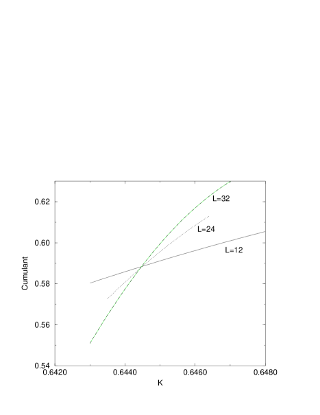
FIG. 1.: Fourth-order cumulant $U_{L}(K)$ versus coupling $K$ for lattice sizes $L$=12, 24, and 32.

If one wishes to obtain higher accurary, then one needs to examine Fig. 1 more carefully and to see that the points where each pair of curves cross are slightly different for different pairs of lattices; in fact the points where the curves cross move slowly to lower couplings for larger system sizes. For the pair which corresponds to our largest lattice sizes $L$=32 and 42, the point where they cross is $K_{c}\approx 0.64455$. In order to extract more precise critical coupling $K_{c}$ from our data, we compare the curves of $U_{L}$ for the two different lattice sizes $L$ and $L^{\prime}=bL$ and then find the location of the intersection of two different curves $U_{L}$ and $U_{L^{\prime}}$. As a result of the residual corrections to the finite size scaling [15], the locations depend on the scale factor $b=L^{\prime}/L$. We used the crossing points of the $L$=12, 14, and, 16 curves with all the other ones with higher $L^{\prime}$ value respectively. Hence we need to extrapolate the results of this method for (ln$b$)${}^{-1}\longrightarrow 0$ using $(U_{bL}/U_{L})_{T=T_{c}}=1$. In Fig. 2 we show the estimate for the critical temperature $T_{c}$. Our final estimate for $T_{c}$ is

$$T_{c}=1.5518(2),K_{c}=0.6444(1).$$ (6)

For comparison, the previous estimates are $T_{c}$=1.54(1)[13, 14] obtained using Monte Carlo simulation and $T_{c}$=1.552(3)[12] obtained using high-temperature series. The latter result obtained with an expansion is surprisingly close to ours.

FIG. 2.: Estimates for $T_{c}$ plotted versus inverse logarithm of the scale factor b=$L^{\prime}/L$. The extrapolation leads to an estimate of $T_{c}$=1.5518(2).

In order to extract the critical exponent $\nu$, we performed finite-size scaling analysis of the slopes of $U_{L}$ versus $L$ near our estimated critical point $K_{c}$. In the finite-size scaling region, the slope of the cumulant at $K_{c}$ varies with system size like $L^{1/\nu}$,

$$\frac{dU_{L}}{dK}\sim L^{1/\nu}.$$ (7)

In Fig. 3 we show results of a finite-size scaling analysis for the slope of the cumulant. We obtained the value of the static exponent $\nu$,

$$\nu=0.670(7).$$ (8)

For comparison, the field theoretical estimate[3] is $\nu$=0.669(2) and a recent experimental measurement gives $\nu$=0.6705(6)[20].

FIG. 3.: Log-log plot of the slopes of $U$ near the crossing point versus $L$. The slope gives an estimate for the critical exponent $\nu$=0.670(7).

In order to obtain the value of the exponent ratio $\gamma/\nu$, we calculated the magnetic susceptibility per spin $\chi$ at the critical coupling $K_{c}$. The finite-size behavior for $\chi$ at the critical point is

$$\chi\sim L^{\gamma/\nu}.$$ (9)

Fig. 4 displays the finite-size scaling of the susceptibility $\chi$ calculated at $K_{c}$=0.6444. ¿From the log-log plot we obtained the value of the exponent ratio $\gamma/\nu$,

$$\gamma/\nu=1.9696(37).$$ (10)

¿From the hyperscaling relation, $d\nu=\gamma+2\beta$, we get the exponent ratio $\beta/\nu$,

$$\beta/\nu=0.515(2).$$ (11)

FIG. 4.: Log-log plot of the susceptibility versus the lattice size $L$ at the critical coupling $K_{c}$=0.6444. The slope gives an estimate for the critical exponent $\gamma/\nu$=1.9696(37).

The equilibrium magnetization $m$ at $K_{c}$ should obey the relation

$$m\sim L^{-\beta/\nu}$$ (12)

for sufficiently larger $L$. In Fig. 5 we show the results of a finite-size scaling analysis for the magnetization $m$. We obtain the value of the exponent ratio $\beta/\nu$,

$$\beta/\nu=0.515(2).$$ (13)

This result agrees very closely to that of Eq. (11) obtained from the susceptibility and the fourth-order cumulant.

FIG. 5.: Log-log plot of the magnetization versus the lattice size $L$ at the critical coupling $K_{c}$=0.6444. The slope gives an estimate for the critical exponent $\beta/\nu$=0.515(3).

$L$	$\chi$	$m$
12	82.39(28)	0.26195(55)
14	111.88(36)	0.24219(43)
16	145.12(59)	0.22567(55)
18	182.91(52)	0.21241(35)
20	224.08(85)	0.20072(49)
22	272.23(60)	0.19163(23)
24	322.35(98)	0.18308(32)
32	571.0(4.0)	0.15833(66)
42	972.0(4.8)	0.13749(40)

TABLE I.: Results for the magnetization and the susceptibility

In conclusion, we determined the critical temperature and the exponents of the planar magnet model with three-component spins using a high-precision MC method, the single-histogram method, and the finite-size scaling theory. Our simulation results for the critical coupling and for the critical exponents are $K_{c}$=0.6444(1), $\nu$=0.670(7), $\gamma/\nu$=0.9696(37), and $\beta/\nu$=0.515(2). Our calculated values for the critical temperature and critical exponents are significantly more accurate that those previously calculated. Comparison of our results with results of MC studies of the 3$D$ $XY$ model with two-component spins[7, 9, 10, 11] shows that both the system with $\vec{S}_{i}=(S^{x}_{i},S^{y}_{i})$ and the planar magnet system with $\vec{S}_{i}=(S^{x}_{i},S^{y}_{i},S^{z}_{i})$ belong to the same universality class.

IV acknowledgements

This work was supported by the National Aeronautics and Space Administration under grant no. NAG3-1841.

REFERENCES

- [1] K.G. Wilson, Phys. Rev. B 4, 3174 (1971).
- [2] P.C. Hohenberg and B.I. Halperin, Rev. Mod. Phys. 49, 435 (1977).
- [3] J.C. Le Guillou and J. Zinn-Justin, Phys. Rev. B 21, 3976 (1980).
- [4] D.Z. Albert, Phys. Rev. B 25, 4810 (1982).
- [5] P. Butera, M. Comi, and A. J. Guttmann, Phys. Rev. B 48, 13987 (1993); R. G. Bowers and G. S. Joyce, Phys. Rev. Lett. 19, 630 (1967).
- [6] Y.-H.Li and S. Teitel, Phys. Rev. B 40, 9122 (1989).
- [7] A. P. Gottlob and M. Hasenbusch, Physica A 201, 593 (1993); A. P. Gottlob, M. Hasenbusch and S. Meyer, Nucl. Phys. B (Proc. Suppl.) 30, 838 (1993).
- [8] N. Schultka and E. Manousakis, Phys. Rev. B 51, 11712 (1995).
- [9] N. Schultka and E. Manousakis, Phys. Rev. B 52, 7528 (1995).
- [10] W. Janke, Phys. Lett. A 148, 306 (1990).
- [11] Martin Hasenbusch and Steffen Meyer, Phys. Lett. B 241, 238 (1990).
- [12] M. Ferer, M.A. Moore, and M. Wortis, Phys. Rev. B 8, 5205 (1973).
- [13] B.V. Costa, A.R. Pereira, and A.S.T. Pires, Phys. Rev. B 54, 3019 (1996).
- [14] S.K. Oh, C.N. Yoon, and J.S. Chung, Phys. Rev. B 56, 13677 (1997).
- [15] K. Binder, Z. Phys. B 43, 119 (1981).
- [16] P. Peczak and D.P. Landau, Phys. Rev. B 47, 14260 (1963).
- [17] U. Wolff, Phys. Rev. Lett. 62, 361 (1989).
- [18] F.R. Brown and T.J. Woch, Phys. Rev. Lett. 58, 2394 (1987).
- [19] A.M. Ferrenberg and R.H. Swendsen, Phys. Rev. Lett. 61, 2635 (1988); , 63, 1195 (1989).
- [20] L.S. Goldner, N. Mulders, and G. Ahlers, J. Low Temp. Phys. 93, 131 (1992).