Hydrodynamics of bacterial motion

Abstract

In this paper we present a hydrodynamic approach to describe the motion of migrating bacteria as a special class of self-propelled systems. Analytical and numerical calculations has been performed to study the behavior of our model in the turbulent-like regime and to show that a phase transition occurs as a function of noise strength. Our results can explain previous experimental observations as well as results of numerical simulations.

I Introduction

Bacterial colony formation has been the subject of recent studies performed by both microbiologists[1, 2, 3, 4, 5] and physicists[6, 7, 8, 9, 10, 11, 12, 13] with the aim to acquire a deeper understanding of the collective behavior of unicellular organisms.

Since bacterial colonies can consist of up to $10^{10}$ microorganisms, one can distinguish several length and time scales when describing their development. At the largest, macroscopic scale (above cca. $10^{-3}$ m) one is concerned about the morphology of the whole colony, which can be often described in terms of fractal geometry [6, 9, 11]. At this length scale, the physical  laws of diffusion govern colony formation, and only certain details of the underlying microscopic dynamics (such as anisotropy [14]) can be amplified up to this scale by various instabilities. Thus these large-scale features could have been successfully understood using relatively simple models which neglect most of the microscopic details. In contrast, when looking at the microscopic length scale of individual bacteria (cca. $10^{-6}$ m), such global physical constraints play a much smaller role and it is the biology which provides us the knowledge of how the microorganisms move, multiplicate and communicate. In this work we focus on the intermediate length and time scales which range from $10^{-5}$ m to $10^{-3}$ m and from $1$ s to $10^{2}$ s. In this regime the proliferation of the bacteria can be neglected, and the most striking observable phenomena are connected to the motion of the organisms.

Bacterial swimming has been well understood in liquid cultures [15, 16, 17], where the interaction between cells is usually negligible and the trajectory of each organism can be described as a biased random walk towards the higher concentration of the chemoattractants, e.g., certain nutrients. In fact, the bacterial motion consists of straight sections separated by short periods of random rotation called tumbling, when the flagellas operate in a quite uncorrelated manner. If an increase of the local concentration of the chemoattractant is detected, bacteria delay tumbling and continue to swim in the same direction. This behavior yields the above mentioned bias towards the chemoattractant. Recent experimental observations [3, 11, 5] revealed that under stress conditions even chemotactic communication occurs in colonies: chemoattractants or chemorepellents are emitted by the bacteria themself, thus controlling the development of various self-organized structures[12].

However, numerous bacterial strains like Proteus mirabilis, Serratia marcenses [2] Bacillus circulans, Archangium violanceum, Chondromyces apiculatus, Clostridium tetani [18] or Bacillus subtilis [10] are also able to migrate on surfaces to ensure their survival under hostile environmental conditions. In all of these examples, irrespective of the cell membrane (Gram $+$ or $-$) and the type of locomotion (swarming or gliding), a significantly coordinated motion can be observed: the randomness, which is a characteristic feature of the swimming of an individual organism, is rather repressed. In particular the swarmer cells of the strain Proteus are very elongated (up to 50$\mu$m) and move parallel to each other [2]. The strain Bacillus circulans obtained its name from the very complex flow trajectories exhibited, which include rotating droplets or rings made up of thousands of bacteria [18, 19]. To some extent similar behavior can be observed in each of the above listed examples, which naturally raises the long standing question as to whether this form of migration requires some external (or self-generated) chemotactic signal or whether simple local cell-cell interactions are sufficient to explain such correlated behavior.

One of the purposes of this paper is to show that the answer to such questions requires taking into account that the bacteria are far-from equilibrium, self-propelled systems. Recent studies have revealed that such systems show interesting and unexpected features: in various traffic models spontaneous jams appear [20, 21] and there is a strong dependence on quenched disorder [22]. Many biological system (such as swarming bacteria, schools of fishes, birds, ants, etc.) can be described as special self-propelled systems with local velocity-velocity interaction introduced by Vicsek et al. [23] and also studied in a lattice gas model [24]. Both of these models revealed transition from disordered to ordered phase. Although most of the models above incorporate some level of discreteness, a continuum approach also has been applied to study the traffic flow problem [21] or to describe the geotactic motion of bacteria [25]. Toner and Tu have shown using renormalization group theory that in a closely related continuum model [26] a long range order can develop even in two dimensions; this is not possible in the equivalent equilibrium models.

In this paper we construct a continuum description for the particularly interesting collective motion in bacterial colonies. First we introduce our model, then we give a theoretical analysis of the problem. In Section IV we present the numerical results and finally in Section V we draw our conclusions.

II The Model

When migrating on surfaces, bacteria usually form a very thin film consisting only of a single or a few layers of cells, thus their motion can be regarded as quasi two-dimensional. Due to the small length scale, the very small Reynolds number yields an overdamped dynamics in which the thermal fluctuations (Brownian noise) and the various surface effects (e.g., surface tension, wetting) dominate the motion. The constrains of the cell-cell interaction must also be taken into account since the elongated migrating bacteria usually align parallel to each other, which results in an effective viscosity that tends to homogenize the velocities as we show later. Bacteria also tend to move close to the substrate which manifests in an effective gravity, flattening the colony.

The particles of the “bacterial fluid” (i.e., the colony) are bacteria surrounded by a droplet of moisture (extracellular fluid, see Fig. 1) which is essential for them both to move and to extract food from the substrate. The volume ($V^{*}$) and the mass ($m^{*}$) of such a particle is considered to be constant, which gives a constant (3D) density $\varrho^{*}=m^{*}/V^{*}$. A typical bacterial colony grown on a surface can be considered as flat, so our fluid will be characterized by the 2D number density $\varrho({\bf r},t)$ and velocity ${\bf v}({\bf r},t)$ fields, where ${\bf r}\in{\rm R}^{2}$ and $t$ is the time. The number density is simply related to the local height of the colony $h$ by $h({\bf r},t)=\varrho({\bf r},t)V^{*}$.

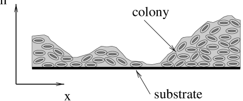
FIG. 1.: Schematic crossection of a bacterial colony.

In contrast to fluid mechanics, here the fluid element consists of only a few “atoms”. Thus random fluctuations do not cancel out and they have to be taken into account by an additional noise term in the equation of motion for the velocity field. The two basic equations governing the dynamics are the continuity equation

$$\partial_{t}\varrho+\nabla(\varrho{\bf v})=0$$ (1)

and the equation of motion, which is a suitable form of the Navier-Stokes equation

$$\partial_{t}{\bf v}+({\bf v}\cdot\nabla){\bf v} = -{1\over\varrho^{*}}\nabla p+\nu\nabla^{2}{\bf v}+{1\over\varrho^{*}}{\bf F}({\bf v})-{1\over\tau}{\bf v}$$ (3)

$$+{\bf\eta}({\bf x},t),$$

where $p$ is the pressure, $\nu$ is the kinematic viscosity, ${\bf F}({\bf v})$ is the intrinsic driving force of biological origin, $\tau$ is the time scale associated with substrate friction and ${\bf\eta}({\bf x},t)$ is an uncorrelated fluctuating force with zero mean and variance $\sigma$ representing the random fluctuations. Let us now go through the terms of Eq. 3.

The pressure is composed of the effective hydrostatic pressure, the capillary pressure, and the externally applied pressure

$$p=\varrho^{*}gh+\gamma\nabla^{2}h+p_{\rm ext}.$$ (4)

If the radius of surface curvature is larger then the capillary length

$$l_{\rm cap}=\sqrt{\gamma\over{\varrho^{*}g}}$$ (5)

then the capillary pressure can be neglected. Since this is normally the case ($l_{\rm cap}\approx 3$ mm for water), we consider only the first term of Eq. 4 in the rest of the paper. The surface tension becomes relevant only at the boundary of the colony where the local curvature is not negligible.

The viscous term in Eq. 3 represents not only the viscosity of the extracellular fluid, but also incorporates the local ordering of the cells. As we show in Appendix A for a simple hard rod model of the cell-cell interaction, the deterministic part of the dynamics of the orientational ordering is described in a similar manner to [23]:

$${{\rm d}\theta_{i}\over{\rm d}t}=\mu\Bigl{(}\langle\theta\rangle_{\epsilon}-\theta_{i}\Bigr{)},$$ (6)

where the orientation of the $i$th rod is denoted by $0<\theta_{i}<\pi$ and $\langle\cdot\rangle_{\epsilon}$ denotes spatial averaging over a ball of radius $\epsilon$. The angle $\theta$ can be readily replaced by ${\bf e}_{\theta}$, a unit vector at angle $\theta$ to the $x$ axis. If the changes in the magnitude of the velocity are small then ${\bf e}_{\theta}$ can be replaced by ${{\bf v}}$ and Eq. 6 yields an interaction term proportional to $\langle{{\bf v}}\rangle_{\epsilon}-{{\bf v}}$.

Taking Taylor series expansions for the velocity and the density fields yields

$$\langle{{\bf v}}\rangle_{\epsilon}-{\bf v} = {\int_{|{\bf\xi}|<\epsilon}\hbox{d}{\bf\xi}\Bigl{(}{{\bf v}}\varrho+({\bf\xi}\nabla){{\bf v}}\varrho+{1\over 2}({\bf\xi}\nabla)^{2}{{\bf v}}\varrho+\dots\Bigr{)}\over\int_{|{\bf\xi}|<\epsilon}\hbox{d}{\bf\xi}\Bigl{(}\varrho+({\bf\xi}\nabla)\varrho+{1\over 2}({\bf\xi}\nabla)^{2}\varrho+\dots\Bigr{)}}-{\bf v}$$ (7)

$$= {\epsilon^{2}\over 6}\Bigl{(}{\nabla^{2}({{\bf v}}\varrho)\over\varrho}-{{\bf v}}{\nabla^{2}\varrho\over\varrho}\Bigr{)}+\dots$$ (8)

$$= {\epsilon^{2}\over 6}\Bigl{(}\nabla^{2}{{\bf v}}+2(\nabla{{\bf v}}){\nabla\varrho\over\varrho}\Bigr{)}+\dots$$ (9)

If the density changes are small, we recover the viscous term of Eq. 3, so it, in fact, includes the self-alignment rule of previous models.

Bacteria tend to maintain their motion continuously by propelling with their flagellas. This rather complex behavior can be taken into account as a constant magnitude force acting in the direction of their velocity

$${\bf F}=\varrho^{*}{c\over\tau}{{{\bf v}}\over{|{{\bf v}}|}},$$ (10)

where $c$ is the speed determined by the balance of the propulsion and friction forces. That is, $c$ would be the speed of a homogeneous fluid.

Combining Eqs. 1, 3, 4 and 10 we obtain the following final form for the equations of the bacterial flow:

$$\partial_{t}h+\nabla(h{\bf v})=0,$$ (11)

and

$$\partial_{t}{\bf v}+({\bf v}\cdot\nabla){\bf v} = -{g}\nabla h+-{1\over\varrho^{*}}\nabla p_{\rm ext}+\nu\nabla^{2}{\bf v}$$ (13)

$$+{c\over\tau}{{{\bf v}}\over{|{{\bf v}}|}}-{1\over\tau}{\bf v}+{\bf\eta}.$$

These equations are similar to those studied in [26] but here we derived them from plausible assumptions based on the underlying microscopic dynamics instead of phenomenological concepts. Nevertheless, the analysis of Toner and Tu also holds for our equations which permits us to use our model as a test of their prediction of the existence of a phase transition.

III Analytical results

For certain simple geometries of the boundary condition it is possible to obtain analytical solutions for the noiseless ($\sigma=0$) stationary state of our model if we suppose incompressibility ($h=const.$). Taking $\partial_{t}\equiv 0$ in Eqs. 11 and 13, the following dimensionless equations are obtained:

$$\nabla^{\prime}{{\bf v}}^{\prime}=0$$ (14)

and

$${{c\tau}\over{\lambda}}({\bf v}^{\prime}\nabla^{\prime}){\bf v}^{\prime}=-{1\over{\varrho^{*}\lambda}}\nabla p_{\rm ext}+{\nabla}^{\prime 2}{\bf v}^{\prime}+{{\bf v}^{\prime}\over{|{{\bf v}}^{\prime}|}}-{{{\bf v}}}^{\prime},$$ (15)

where ${{\bf v}}^{\prime}={{\bf v}}/c$, $\lambda=\sqrt{\nu\tau}$ and the $\nabla^{\prime}$ operator derivates with respect to ${\bf r}^{\prime}={\bf r}/\lambda$. For the sake of simplicity we drop the prime in the rest of this section.

First let us consider the simplest geometry when the system is defined on an infinite plane. In this case the stationary state is trivially

$$|{{\bf v}}({\bf r})|=1,$$ (16)

where the orientation of ${{\bf v}}$ is arbitrary, but independent of the spatial position. In this state there is a sustained non-zero net flux of the fluid so it is regarded to be ordered. In the next section we examine numerically how increasing the noise level yields a disordered state where there is no net flux present.

Another simple, but practically more relevant boundary condition is realized when the system is confined to a circular area of radius $R$. In contrary to the previous example this is a finite geometry which in turn means that in the stationary state no net flux is possible. Thus the flow field must include vortices and we show that a single vortex is indeed a possible stationary configuration of the system.

Let us assume that the velocity field, expressed in polar coordinates $(r,\phi)$, is a function only of $r$:

$${{\bf v}}=v(r)~{}{\bf e}_{\phi},$$ (17)

where ${\bf e}_{\phi}$ is the tangential unit vector. Taking the expression of the nabla operator in polar coordinates, one can easily see that Eq. 14 is satisfied for any velocity profile $v(r)$. Substituting Eq. 17 into Eq. 15 yields two ordinary differential equations:

$$0=r^{2}{{{\rm d}^{2}v}\over{\rm d}r^{2}}+r{{{\rm d}v}\over{\rm d}r}-v(1+r^{2})+r^{2},$$ (18)

and

$$-{1\over r^{2}}v^{2}=-{1\over{\varrho^{*}\lambda}}{{\partial p_{\rm ext}}\over\partial r}.$$ (19)

The first equation gives the velocity profile while the second determines the pressure to be applied for maintaining the constant height ($h=$const.) condition.

The boundary conditions for the velocity profile are either $v(0)=0$ and $v(R^{\prime})=0$ (closed boundary at $r=R^{\prime}=R/\lambda$) or $v(0)=0$ and ${{{\rm d}v}\over{{\rm d}r}}(R^{\prime})=0$ (free boundary at $r=R^{\prime}$). The homogeneous solution of the equation of motion with the above boundary conditions is given by $I_{1}(r)$, the modified Bessel function of order one. The particular solution is $-{\pi\over 2}L_{1}(r)$, where $L_{1}$ is the modified Struve function of order one [27]. Thus the velocity profile of the single vortex stationary state in a noiseless system with circular boundary is

$$v(r)=\alpha I_{1}(r)-{\pi\over 2}L_{1}(r).$$ (20)

The parameter $\alpha$ should be chosen to satisfy the boundary condition at $r=R^{\prime}$. In Fig. 2 we show velocity profiles for different values of $\lambda$ having $R=1$ fixed and imposing closed boundary condition. The maximal velocity decreases for decreasing $R/\lambda$ ratio (Fig. 3); thus the system behaves more similar to the usual (not self-propelled) systems where $v(r)\equiv 0$. In this respect $R/\lambda$ is a measure of the self-propulsion. From Fig. 2 it is also clear that the minimal size of a vortex is $\lambda$ so if $R/\lambda\gg 1$ then many vortices are likely to be present in the system. This phenomenon is analogous to the appearance of turbulent motion in fluid dynamics and thus $R/\lambda$ can be regarded as a quantity analogous to the Reynolds number:

$${\rm Re}^{\prime}={R\over\lambda}.$$ (21)

Another dimensionless quantity characterizing the flow is $c\tau/\lambda$ which gives the relative strength of the inertial forces compared the viscous ones. This quantity can be regarded as an internal Reynolds number

$${\rm Re}^{\prime\prime}={c\tau\over\lambda}.$$ (22)

In our simulations we always had ${\rm Re}^{\prime\prime}\ll{\rm Re}^{\prime}$.

FIG. 2.: Velocity profiles in a vortex for various values of ${\rm Re}^{\prime}$ (bottom curve: ${\rm Re}^{\prime}=1$, top curve: ${\rm Re}^{\prime}=16$).

FIG. 3.: Position (solid line) and value (dashed line) of the maximal velocity for the profiles on Fig. 2 as a function of ${\rm Re}^{\prime}$. At the maximal velocity, open boundary condition (${\rm d}v/{\rm d}r=0$) is satisfied.

IV Numerical results

For further investigations we used numerical solutions of Eq. 11 and Eq. 13. To study the closed circular geometry we implemented our model on a hexagonal region of a triangular lattice with closed boundary conditions. We used a simple explicit integration scheme to solve numerically the equations.

We started our simulations from a uniform density and a random velocity distribution. Figure 4 shows the stationary state for the high viscosity ($\lambda\simeq 3.16$) and high compressibility ($g=750$) case, corresponding to ${\rm Re}^{\prime}\simeq 4.4$. The length and direction of the arrows show the velocity, while the thickness is proportional to the local density of the fluid. In Fig. 5 we present the radial velocity distribution for the vortex shown in Fig. 4 and the velocity profile given by our calculations (Eq. 20). Rather good agreement is seen; the differences are due to the fact that our numerical system is not perfectly circular. We have also performed velocity profile analysis for two vortices from [19]. The data and the fitted curves are displayed in Fig. 6. Again, reasonable agreement is seen which means that Eqs. 11 and 13 give a correct continuous description for this particular example of self-propelled systems.

FIG. 4.: A numerically generated vortex for ${\rm Re}^{\prime}\simeq 4.4$ and $g=750$. The length of the arrows is proportional to the local velocity, while their thickness is proportional to the density.

FIG. 5.: The measured (circles) and the theoretical (solid line) velocity profile for the vortex in Fig. 4.

FIG. 6.: Velocity profile data for two vortices taken from [19] (circles and squares) and fitted profiles using Eq. 20.

In the case of real bacteria one hardly can observe a perfect vortex, so we tuned the parameters to see the behavior of the model far from stationarity. Lowering the value of the compressibility $g$, we observed temporally periodic structures instead of a constant velocity profile vortex. Figure 7 shows such a configuration. The density at the lower left part of the system is higher than at the top right part. As the system evolves in time the whole flow pattern rotates anti-clockwise, thus this state has non-zero net flux which oscillates in time. Similar behavior also has been reported for certain bacterial colonies[10] .

FIG. 7.: Non-stationary configuration at ${\rm Re}^{\prime}=4.4,g=300$.

Another interesting case occurs when the compressibility is high and the viscosity is low, which corresponds to high values of ${\rm Re}^{\prime}$. In this limit we observed a long lifetime multi-vortex state (Fig. 8). For the parameter values we use, these vortices eventually disappeared leaving behind a single vortex. We conjecture that there exists a ${\rm Re}^{\prime}_{c}$ above which the multi-vortex state does not die out, this would correspond to the turbulent state of the normal hydrodynamics.

FIG. 8.: Multiple vortex state at ${\rm Re}^{\prime}=25.3,g=128$.

We also performed simulations in the open planar geometry. In this case our numerical system was confined to a square with periodic boundary conditions. Our goal was to find if there exists the phase transition as a function of the noise strength $\sigma$. To do this we first defined an order parameter

$$\Phi=\langle|{\bf v}|\rangle,$$ (23)

where $\langle\cdot\rangle$ denotes spatial average over the entire system. If $\Phi=0$ there is no net current and the system is in disordered state. If $\Phi>0$ some level of order is present. We have performed long time ($>10^{7}$ Monte-Carlo steps) runs for two different system sizes (L=24 and 48) to check the presence of the transition. Figure 9 shows the results obtained which strongly suggests that there is a transition around $\sigma\approx 6.5$. This value is by far not universal as it depends on the actual values of parameters used in the simulations. However, the extraction of the critical exponents would require much larger computational efforts (i.e., larger system sizes).

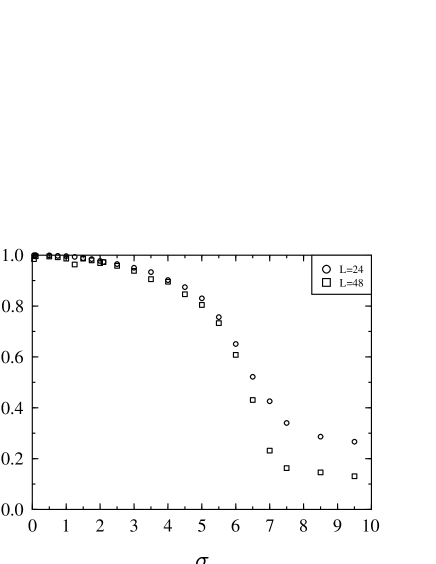
FIG. 9.: The order parameter $\Phi$ as a function of the noise strength $\sigma$.

V Conclusion

We have investigated a continuous model for cooperative motion of bacteria. For simple geometries and specific parameters we were able to obtain analytical results for the velocity profile of vortices often observable on intermediate length scales in various bacterial colonies. Our results are in quantitative agreement with biological observations [18] and with previous simulations [19]. We also showed that there exists a transition [26] from an ordered to a disordered phase as a function of noise strength.

In its present form our model does not give a model for the pattern formation of bacterial colonies. However, it is rather straightforward to include surface tension and wetting effects in their full detail [28] to handling the dynamics of the colony border. Including proliferation, the presented model can be also expanded towards larger time and length scales to study the fingering instabilities. It is also possible to introduce chemotactic response which would allow long range interactions to build up.

Further work needs to be done to characterize the turbulent regime (which is mostly observed in swarming colonies) and to relate the effective parameters used in our model to the real world quantities such as food or agar concentration.

VI Acknowledgments

The authors thank E. Ben-Jacob, H. Herrmann and T. Vicsek for useful discussions and comments. This work was supported by contracts T019299 and T4439 of the Hungarian Science Foundation (OTKA) and by the “A Magyar Tudományért” foundation of the Hungarian Credit Bank.

A Simple geometrical model for the orientational ordering of cells

In this appendix we show that the simple geometrical constrains originated from the rod-like shape of bacteria can motivate the local orientational ordering introduced in Sec. II. Microscopic observations of high density cell cultures reveal that the orientational order emerges since bacteria tend not to “intersect” each other: usually bacteria form well defined layers in which they are parallel aligned. To investigate quantitatively this phenomenon let us consider a system of rods with unit length and negligible width, covering the plane with a uniform average density $\varrho$. Here we focus on the local orientational order only and neglect the translational movement of the cells. Thus let us assume that the only interaction in the system is the intersection of the rods, and the overdamped dynamics of the system is determined by two effects, a relaxation process minimizing the total number of intersections $U$ and a random Brownian fluctuation as

$${{\rm d}\theta_{i}\over{\rm d}t}=-\lambda{{\partial}\over{\partial}\theta_{i}}U(\theta_{1},\theta_{2},\dots)+\xi_{i}\hbox{~{}~{}mod~{}~{}}\pi,$$ (A1)

where the direction of the $i$-th rod is denoted by $\theta_{i}$ and $\xi_{i}$ is an uncorrelated noise: $\langle\xi_{i}(t)\xi_{j}(t^{\prime})\rangle=C\delta_{ij}\delta(t-t^{\prime})$. As the rods are not directed, $0<\theta_{i}<\pi$. The quantity $U$ can be written as a sum of “pair potentials” $V_{ij}$:

$$U(\theta_{1},\theta_{2},..)={1\over 2}\sum_{i\not=j}V_{ij}({{\bf x}}_{i},\theta_{i},{{\bf x}}_{j},\theta_{j}),$$ (A2)

where $V_{ij}$ equals $1$ if the rods $i$ and $j$ intersect and $0$ otherwise.

As a mean-field approximation, we introduce the probability density function $P(\theta)$, which gives the probability density of the event that the direction of a randomly selected rod is in the interval $[\theta,\theta+{\rm d}\theta]$. We are interested in the local (short range) ordering; thus the spatial homogeneity of $P$ is assumed. Now $U(\theta)$, the expected number of intersections of a rod directed at angle $\theta$, can be expressed as

$$U(\theta)=\varrho\int_{V}{\rm d}^{2}{{\bf x}}^{\prime}\int_{0}^{\pi}{\rm d}\theta^{\prime}V({{\bf x}}_{i},\theta,{{\bf x}}^{\prime},\theta^{\prime})P(\theta^{\prime}),$$ (A3)

since $\varrho P(\theta)$ gives the probability density for the existence of a rod pointing in the direction $\theta$ at any position. Due to the translational and rotational invariance of the system, $U(\theta)$ is given in the form of

$$U(\theta)=\varrho\int_{0}^{\pi}{\rm d}\theta^{\prime}P(\theta^{\prime})\int_{V}{\rm d}^{2}{{\bf x}}^{\prime}V(0,0,{{\bf x}}^{\prime},\theta^{\prime}-\theta).$$ (A4)

As $\int{\rm d}^{2}{{\bf x}}^{\prime}V(0,0,{{\bf x}}^{\prime},\theta^{\prime}-\theta)$ gives the area of a parallelogram shown in Fig. 10, (A4) can be written as

$$U(\theta)=\varrho\int_{0}^{\pi}{\rm d}\theta^{\prime}P(\theta^{\prime})|\sin(\theta^{\prime}-\theta)|.$$ (A5)

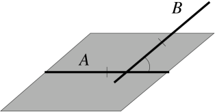
FIG. 10.: The rods $A$ and $B$ with a given orientation intersect each other if the center of rod $B$ is inside of the displayed parallelogram attached to rod $A$.

The time evolution of the probability density function is given by the Fokker-Planck equation obtained from (A1):

$${{\partial}P\over{\partial}t}={{\partial}\over{\partial}\theta}\Bigl{(}\lambda P{{\partial}\over{\partial}\theta}U+{C\over 2}{{\partial}\over{\partial}\theta}P\Bigr{)}.$$ (A6)

The steady state solution of Eq. A6 assuming detailed balance satisfies

$$\lambda P{{\partial}U\over{\partial}\theta}+{C\over 2}{{\partial}P\over{\partial}\theta}=0,$$ (A7)

yielding

$$P(\theta)=P_{0}\exp\Bigl{(}-{2\lambda U(\theta)\over C}\Bigr{)},$$ (A8)

where the normalization for $P(\theta)$ is provided by the prefactor $P_{0}$.

Let us measure $\theta$ compared to the spontaneously selected orientation $\langle\theta\rangle$. For small deviations $U(\theta)$ can be expanded in a Taylor series as

$$U(\theta)\approx{A\over 2}\theta^{2}+O(\theta^{4}).$$ (A9)

Now, from Eqs. A8 and A5 the coefficient $A$ can be calculated for given $\varrho$, $\lambda$ and $D$. Substituting Eq. A9 into Eq. A8 gives

$$P(\theta)\approx P_{0}e^{-A\lambda\theta^{2}/C},$$ (A10)

with

$$P_{0}=\sqrt{A\lambda\over\pi C}.$$ (A11)

For $\theta,\theta^{\prime}\ll 1$ the $|\sin(\theta^{\prime}-\theta)|$ term of Eq. A5 can be linearized both in $\theta$ and $\theta^{\prime}$:

$$U(\theta) = \varrho\theta\left(\int_{-\pi/2}^{\theta}d\theta^{\prime}P(\theta^{\prime})-\int_{\theta}^{\pi/2}d\theta^{\prime}P(\theta^{\prime})\right)$$ (A13)

$$-\left(\int_{-\pi/2}^{\theta}d\theta^{\prime}P(\theta^{\prime})\theta^{\prime}-\int_{\theta}^{\pi/2}d\theta^{\prime}P(\theta^{\prime})\theta^{\prime}\right).$$

After some algebraic manipulations the above expression can be simplified to

$$U(\theta)=2\varrho\int_{0}^{\theta}{\rm d}\theta^{\prime}P(\theta^{\prime})(\theta-\theta^{\prime})\approx\varrho P_{0}\theta^{2}$$ (A14)

yielding the consistency condition $\varrho P_{0}=A/2$. Thus, in this mean field approximation

$${{\rm d}\theta_{i}\over{\rm d}t}=-{\lambda\over\pi C}(\theta_{i}-\langle\theta\rangle_{i}),$$ (A15)

that is we recover Eq. 6. The angle $\theta$ can be readily replaced by ${\bf e}_{\theta}$, a unit vector at angle $\theta$ to the $x$ axis. If the changes in the magnitude of the velocity are small then ${\bf e}_{\theta}$ can be replaced by ${{\bf v}}$ and we recover the self-aligning interaction Eq. 6.

REFERENCES

- [1] Shapiro, J. A. 1988. Bacteria as multicellular organisms. Sci. Amer. 256:62-69.
- [2] Allison, C., and C. Hughes 1991. Bacterial swarming: an example of prokrayotic differentiation and multicellular behavior. Sci. Progress 75:403-422.
- [3] Budrene, E. O., and H. C. Berg. 1991. Complex patterns formed by motile cells of Esherichia coli. Nature 349:630-633.
- [4] Shapiro, J. A. 1995. The significances of bacterial colony patterns. BioEssays 17:597-607.
- [5] Blat, Y., and M. Eisenbach. 1995. Tar-dependent and -independent pattern formation by Salmonella typhimurium. J. Bact. 177:1683-1691.
- [6] Fujikawa, H., and M. Matsushita. 1989. Fractal growth of Bacillus subtilis on agar plates. J. Phys. Soc. Jap. 58:3875-3878
- [7] Matsushita, M., and H. Fujikawa. 1990. Diffusion-limited growth in bacterial colony formation. Physica A 168:498-506.
- [8] Ben-Jacob, E., H. Shmueli, O. Shochet and A. Tenenbaum. 1992. Adaptive self-organization during growth of bacterial colonies. Physica A 187:378-424.
- [9] Matsuyama, T., R. M. Harshey, and M. Matsushita. 1993. Self-similar colony morphogenesis by bacteria as the experimental model of fractal growth by a cell population. Fractals 1:302-311.
- [10] Ben-Jacob, E., A. Tenenbaum, O. Shochet and O. Avidan. 1994. Holotransformations of bacterial colonies and genome cybernetics. Physica A 202:1-47.
- [11] Ben-Jacob, E., O. Shochet, A. Tenenbaum, I. Cohen, A. Czirók and T. Vicsek. 1994. Generic modeling of cooperative growth patterns in bacterial colonies. Nature 386:46-49 and Fractals 2:15-44.
- [12] Ben-Jacob, E., I. Cohen, O. Shochet, I. Aronson, H. Levine and L. Tsimiring. 1995. Complex bacterial patterns. Nature 373:566-567.
- [13] Ben-Jacob, E., I. Cohen, O. Shochet, A. Tenenbaum, A. Czirók and T. Vicsek. 1995. Cooperative formation of chiral patterns during growth of bacterial colonies. Phys. Rev. Lett. 75:2899-2902.
- [14] Ben-Jacob, E., O. Shochet, A. Tenenbaum, I. Cohen, A. Czirók and T. Vicsek. 1996. Response of bacterial colonies to imposed anisotropy. Phys. Rev. E. 53:1835-1841.
- [15] Adler, J. 1969. Chemotaxis in bacteria. Science 166:708-716.
- [16] Berg, H. C., and E. M. Purcell. 1977. Physics of chemoreception. Biophys. J. 20:193-219.
- [17] Lackie J. M. (ed.). 1981. Biology of the chemotactic response. Cambridge University Press, Cambridge, England.
- [18] Wolf, G. (ed.). 1967. Encyclopaedia Cinematographica: Microbiology. Institut für den Wissenschaftlichen Film, Göttingen.
- [19] Czirók, A., E. Ben-Jacob, I. Cohen and T. Vicsek. 1996. Bacterial colony formation via self generated vortices. Phys. Rev. E 54, 1791 (1996).
- [20] Nagel, K., and H. J. Herrmann. 1993. Deterministic models for traffic jams. Physica A 199:254-269.
- [21] Kerner, B. S., and P. Konhäuser. 1993. Cluster effect in originally homogeneous traffic flow. Phys. Rev. E 48:R2335-R2338.
- [22] Csahók, Z., and Vicsek, T. 1994. Traffic models with disorder. J. Phys. A 27:L591-L596.
- [23] Vicsek, T., Czirók, A., Ben-Jacob, E., Cohen, I., and Shochet, O. 1995. Novel type of phase transition in a system of self-driven particles. Phys. Rev. Lett. 75:1226-1229, (1995).
- [24] Csahók, Z., and Vicsek, T. 1995. Lattice-gas model for collective biological motion. Phys. Rev. E 52:5297-5303.
- [25] Childress, S. 1981. Mechanics of swimming and flying, Chapter 12. Cambridge University Press.
- [26] Toner, J., and Tu, Y. 1995. Long-range order in a two-dimensional dynamical XY model: how birds fly together. Phys. Rev. Lett. 75:4326-4329.
- [27] Abramowitz, M., and I. A. Stegun (eds.). 1970. Handbook of Mathematical Functions. Dover Publication, NY.
- [28] de Gennes, P. G. 1985. Wetting: statics and dynamics. Rev. Mod. Phys. 57:825-863.