Flux Confinement in Mesoscopic Superconductors

Abstract

We report on flux confinement effects in superconducting submicron line, loop and dot structures. The main idea of our study was to vary the boundary conditions for confinement of the superconducting condensate by taking samples of different topology and, through that, modifying the lowest Landau level $E_{LLL}(H)$. Since the critical temperature versus applied magnetic field $T_{c}(H)$ is, in fact, $E_{LLL}(H)$ measured in temperature units, it is varied as well when the sample topology is changed. We demonstrate that in all studied submicron structures the shape of the $T_{c}(H)$ phase boundary is determined by the confinement topology in a unique way.

(Received 9 November 1998)

1 Introduction

Recent impressive progress in nanostructuring (e-beam lithography, single atom manipulation with a scanning tunneling microscope tip, etc.) has made it possible to control the quantization effects in nanostructures by varying their size and topology. The most commonly used so far for this purpose are semiconducting structures, where an elegant approach developed by Landauer [1] relates directly mesoscopic transport to the quantum transition probability, which is determined by the specific configuration of quantum levels and available tunneling barriers. Changing the confinement potential via nanostructuring allows to tune both the quantum levels and the tunneling probabilities. Extended by Büttiker [2] to the multi-terminal measurement geometry, the Landauer-Büttiker formalism has been widely and very successfully used in the interpretation of numerous mesoscopic experiments [3].

In comparison to the semiconducting and normal systems, superconducting structures have been studied much less so far. In this report, it is worth first to ask a few simple questions like: why do we want to make such structures, what interesting new physics do we expect, and why do we want to focus on superconducting (and not, for example, normal metallic) nanostructured materials?

First of all, by making low dimensional systems, one creates an artificial potential in which charge carriers or flux lines are confined. The confinement length scale $L_{A}$ of an elementary ”plaquette” A, gives roughly the expected energy scale $E=\hbar^{2}\pi^{2}n^{2}/(2mL_{A}^{2})$. The concentration of charge carriers or flux lines can be controlled by varying the gate voltage in two-dimensional (2D) electron gas systems [4] or the applied magnetic field in superconductors [5]. In this situation, different commensurability effects between the fixed number of elements A in an array and a tunable number of charge or flux carriers are observed.

Secondly, modifying the sample topology in those systems creates a unique possibility to impose the desired boundary conditions, and thus almost ”impose” the properties of the sample. A Fermi liquid or a superconducting condensate confined within such a system will be subjected to severe constraints and, as a result, the properties of these systems will be strongly affected by the boundary conditions.

While a normal metallic system should be considered quantum-mechanically by solving the Schrödinger equation:

$$\frac{1}{2m}\left(-\imath\hbar\vec{\nabla}-e\vec{A}\right)^{2}\Psi+U\>\Psi=E\>\Psi\>,$$ (1)

a superconducting system is described by the two coupled Ginzburg-Landau (GL) equations:

$$\frac{1}{2m^{\star}}(-i\hbar\vec{\nabla}-e^{\star}\vec{A})^{2}\Psi_{s}+\beta|\Psi_{s}|^{2}\Psi_{s}=-\alpha\Psi_{s}$$ (2)

$$\vec{j_{S}}=\vec{\nabla}\times\vec{h}=\frac{e^{\star}}{2m^{\star}}\left[\Psi_{s}^{\star}(-\imath\hbar\vec{\nabla}-e^{\star}\vec{A})\Psi_{s}+\Psi_{s}(\imath\hbar\vec{\nabla}-e^{\star}\vec{A})\Psi_{s}^{\star}\right]\>,$$ (3)

with $\vec{A}$ the vector potential which corresponds to the microscopic field $\vec{h}=rot\vec{A}/\mu_{0}$, $U$ the potential energy, $E$ the total energy, $\alpha$ a temperature dependent parameter changing sign from $\alpha>0$ to $\alpha<0$ as $T$ is decreased through $T_{c}$, ${\beta}$ a positive temperature independent constant, $m^{\star}$ the effective mass which can be chosen arbitrarily and is generally taken as twice the free electron mass $m$.

Note that the first GL equation (Eq. (2)), with the nonlinear term $\beta|\Psi_{s}|^{2}\Psi_{s}$ neglected, is the analogue of the Schrödinger equation (Eq. (1)) with $U$ = 0, when making the following substitutions: $\Psi_{s}(\Psi$), $e^{\star}(e)$, $-\alpha(E)$ and $m^{\star}(m)$. The superconducting order parameter $\Psi_{s}$ corresponds to the wave function $\Psi$; the effective charge $e^{\star}$ in the GL equations is $2e$, i.e. the charge of a Cooper pair; the temperature dependent GL parameter $\alpha$

$$-\alpha=\frac{\hbar^{2}}{2m^{\star}\>\xi^{2}(T)}$$ (4)

plays the role of $E$ in the Schrödinger equation. Here $\xi(T)$ is the temperature dependent coherence length:

$$\xi(T)=\xi(0)\,\left(1-\frac{T}{T_{c0}}\right)^{-1/2}.$$ (5)

The boundary conditions for interfaces between normal metal-vacuum and superconductor-vacuum are, however, different (Fig. 1):

$$\left.\Psi\Psi^{\star}\right|_{b}=0$$ (6)

$$\left.(-\imath\hbar\vec{\nabla}-e^{\star}\vec{A})\Psi_{s}\right|_{\perp,b}=0$$ (7)

i.e. for normal metallic systems the density is zero, while for superconducting systems, the gradient of $\Psi_{s}$ (for the case $\vec{A}=0$) has no component perpendicular to the boundary. As a consequence, the supercurrent cannot flow through the boundary. The nucleation of the superconducting condensate is favored at the superconductor/ vacuum interfaces, thus leading to the appearance of superconductivity in a surface sheet with a thickness $\xi(T)$ at the third critical field $H_{c3}(T)$.

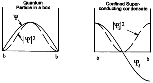
Fig.  1: Boundary conditions for interfaces between normal metal-vacuum and superconductor-vacuum.

For bulk superconductors the surface-to-volume ratio is negligible and therefore superconductivity in the bulk is not affected by a thin superconducting surface layer. For submicron superconductors with antidot arrays, however, the boundary conditions (Eq. (7)) and the surface superconductivity introduced through them, become very important if $L_{A}\leq\xi(T)$. The advantage of superconducting materials in this case is that it is not even necessary to go down to the nanometer scale (like for normal metals), since for $L_{A}$ of the order of 0.1-1.0 $\mu m$ the temperature range where $L_{A}\leq\xi(T)$, spreads over $0.01-0.1~{}K$ below $T_{c}$ due to the divergence of $\xi(T)$ at $T\rightarrow T_{c0}$ (Eq. (5)).

In principle, the mesoscopic regime $L_{A}\leq\xi(T)$ can be reached even in bulk superconducting samples with $L_{A}\sim$ $1~{}cm$, since $\xi(T)$ diverges. However, the temperature window where $L_{A}\leq\xi(T)$ is so narrow, not more than $\sim$ $1~{}nK$ below $T_{c0}$, that one needs ideal sample homogeneity and a perfect temperature stability.

In the mesoscopic regime, $L_{A}\leq\xi(T)$, which is easily realized in (perforated) nanostructured materials, the surface superconductivity can cover the whole available space occupied by the material, thus spreading superconductivity all over the sample. It is then evident that in this case surface effects play the role of bulk effects.

Using the similarity between the linearized GL equation (Eq. (2)) and the Schrödinger equation (Eq. (1)), we can formalize our approach as follows: since the parameter -$\alpha$ (Eqs. (2) and (4)) plays the role of energy $E$ (Eq. (1)), then the highest possible temperature $T_{c}(H)$ for the nucleation of the superconducting state in the presence of a magnetic field $H$ always corresponds to the lowest Landau level $E_{LLL}(H)$ found by solving the Schrödinger equation (Eq. (1)) with ”superconducting” boundary conditions (Eq. (7)).

Figure 2 illustrates the application of this rule to the calculation of the upper critical field $H_{c2}(T)$: indeed, if we take the well-known classical Landau solution for the lowest level in bulk samples $E_{LLL}(H)=\hbar\omega/2$, where $\omega=e^{\star}\mu_{0}H/m^{\star}$ is the cyclotron frequency. Then, from -$\alpha=E_{LLL}(H)$ we have

$$\frac{\hbar^{2}}{2m^{\star}\>\xi^{2}(T)}=\left.\frac{\hbar\omega}{2}\right|_{H=H_{c2}}$$ (8)

and with the help of Eq. (4), we obtain

$$\mu_{0}H_{c2}(T)=\frac{\Phi_{0}}{2\pi\xi^{2}(T)}$$ (9)

with $\Phi_{0}=h/e^{\star}=h/2e$ the superconducting flux quantum.

Fig.  2: Landau level scheme for a particle in a magnetic field. From the lowest Landau level $E_{LLL}(H)$ the second critical field $H_{c2}(T)$ is derived (solid line).

In nanostructured superconductors, where the boundary conditions (Eq. (7)) strongly influence the Landau level scheme, $E_{LLL}(H)$ has to be calculated for each different confinement geometry. By measuring the shift of the critical temperature $T_{c}(H)$ in a magnetic field, we can compare the experimental $T_{c}(H)$ with the calculated level $E_{LLL}(H)$ and thus check the effect of the confinement topology on the superconducting phase boundary for a series of nanostructured superconducting samples. The transition between normal and superconducting states is usually very sharp and therefore the lowest Landau level can be easily traced as a function of applied magnetic field. Except when stated explicitly, we have taken the midpoint of the resistive transition from the superconducting to the normal state, as the criterion to determine $T_{c}(H)$.

2 Flux confinement in individual structures: line, loop and dot

In this section we present the experimental $T_{c}(H)$ phase boundary measured in superconducting aluminum mesoscopic structures with different topologies with the same width of the lines ($w=0.15\>\mu m$) and film thickness ($t=25\>nm$). The magnetic field $H$ is always applied perpendicular to the structures.

2.1 Line structure

In Fig. 3a the phase boundary $T_{c}(H)$ of a mesoscopic line is shown. The solid line gives the $T_{c}(H)$ calculated from the well-known formula [6]:

$$T_{c}(H)=T_{c0}\left[1-\frac{\pi^{2}}{3}\left(\frac{w\>\xi(0)\mu_{0}H}{\Phi_{0}}\right)^{2}\right]$$ (10)

which, in fact, describes the parabolic shape of $T_{c}(H)$ for a thin film of thickness $w$ in a parallel magnetic field. Since the cross-section, exposed to the applied magnetic field, is the same for a film of thickness $w$ in a parallel magnetic field and for a mesoscopic line of width $w$ in a perpendicular field, the same formula can be used for both configurations [7]. Indeed, the solid line in Fig 3a is a parabolic fit of the experimental data with Eq. (10) where $\xi(0)=110\>nm$ was obtained as a fitting parameter. The coherence length obtained using this method, coincides reasonably well with the dirty limit value $\xi(0)=0.85(\xi_{0}\ell)^{1/2}=132\>nm$ calculated from the known BCS coherence length $\xi_{0}=1600\>nm$ for bulk Al [8] and the mean free path $\ell=15\>nm$, estimated from the normal state resistivity $\rho$ at $4.2\>K$ [9].

We can use also another simple argument to explain the parabolic relation $T_{c}(H)\propto H^{2}$, since the expansion of the energy $E(H)$ in powers of $H$, as given by the perturbation theory, is [10]:

$$E(H)=E_{0}+A_{1}LH+A_{2}SH^{2}+\cdots$$ (11)

where $A_{1}$ and $A_{2}$ are constant coefficients, the first term $E_{0}$ represents the energy levels in zero field, the second term is the linear field splitting with the orbital quantum number $L$ and the third term is the diamagnetic shift with $S$, being the area exposed to the applied field.

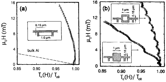
Fig.  3: The measured superconducting/normal phase boundary as a function of the reduced temperature $T_{c}(H)/T_{c0}$ for a) the line structure, and b) the loop and dot structure. The solid line in (a) is calculated using Eq. (10) with $\xi(0)=110\>nm$ as a fitting parameter. The dashed line represents $T_{c}(H)$ for bulk Al.

For the topology of the line with a width $w$ much smaller than the Larmor radius $r_{H}\gg w$, any orbital motion is impossible due to the constraints imposed by the boundaries onto the electrons inside the line. Therefore, in this particular case $L=0$ and $E(H)=E_{0}+A_{2}SH^{2}$, which immediately leads to the parabolic relation $T_{c}\propto H^{2}$. This diamagnetic shift of $T_{c}(H)$ can be understood in terms of a partial screening of the magnetic field $H$ due to the non-zero width of the line [11].

2.2 Loop structure

The $T_{c}(H)$ of the mesoscopic loop, shown in Fig. 3b, demonstrates very distinct Little-Parks (LP) oscillations [12] superimposed on a monotonic background. A closer investigation leads to the conclusion that this background is very well described by the same parabolic dependence as the one which we just discussed for the mesoscopic line [7] (see the solid line in Fig. 3a). As long as the width of the strips $w$, forming the loop, is much smaller than the loop size, the total shift of $T_{c}(H)$ can be written as the sum of an oscillatory part and the monotonic background given by Eq. (10) [7, 13]:

$$T_{c}(H)=T_{c0}\left[1-\frac{\pi^{2}}{3}\left(\frac{w\>\xi(0)\mu_{0}H}{\Phi_{0}}\right)^{2}-\frac{\xi^{2}(0)}{R^{2}}\left(n-\frac{\Phi}{\Phi_{0}}\right)^{2}\right]$$ (12)

where $R^{2}=R_{1}\>R_{2}$ is the product of inner and outer loop radius, and the magnetic flux threading the loop $\Phi=\pi R^{2}\mu_{0}H$. The integer $n$ has to be chosen so as to maximize $T_{c}(H)$ or, in other words, selecting $E_{LLL}(H)$.

The LP oscillations originate from the fluxoid quantization requirement, which states that the complex order parameter $\Psi_{s}$ should be a single-valued function when integrating along a closed contour

$$\oint\vec{\nabla}\varphi\cdot dl=n\>2\pi\;\;\;\;\;\;\;\;\;\;\;\;\;\;\;\;n=\cdots\>,-2,-1,0,1,2,\>\cdots$$ (13)

where we have introduced the order parameter $\Psi_{s}=|\Psi_{s}|\exp\>(\imath\varphi)$. Fluxoid quantization gives rise to a circulating supercurrent in the loop when $\Phi\neq n\Phi_{0}$, which is periodic with the applied flux $\Phi/\Phi_{0}$.

Using the sample dimensions and the value for $\xi(0)$ obtained for the mesoscopic line (with the same width $w=0.15\>\mu m$), the $T_{c}(H)$ for the loop can be calculated from Eq. (12) without any free parameter. As shown in Fig. 3b, the agreement with the experimental data is very good.

Another interesting feature of the mesoscopic loop or other structures is the unique possibility they offer for studying nonlocal effects [14]. In fact, a single loop can be considered as a 2D artificial quantum orbit with a fixed radius, in contrast to Bohr’s description of atomic orbitals. In the latter case the stable radii are found from the quasiclassical quantization rule, stating that only an integer number of wavelengths can be set along the circumference of the allowed orbits. For a superconducting loop, however, supercurrents must flow, in order to fulfill the fluxoid quantization requirement (Eq. (13)), thus causing oscillations of $T_{c}$ versus $H$.

In order to measure the resistance of a mesoscopic loop, electrical contacts have, of course, to be attached to it, and as a consequence the confinement geometry is changed. This ”disturbing” or ”invasive” aspect can now be exploited for the study of nonlocal effects [14]. Due to the divergence of the coherence length $\xi(T)$ at $T=T_{c0}$ (Eq. (5)) the coupling of the loop with the attached leads is expected to be very strong for $T\rightarrow T_{c0}$.

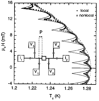
Fig.  4: Local ($V_{1}/V_{2}$) and nonlocal phase boundary ($V_{1}/V_{3}$ or $V_{2}/V_{4}$) measurements. The transport current flows through $I_{1}/I_{2}$. The solid and dashed lines correspond to the theoretical $T_{c}(H)$ of an isolated loop and a one-dimensional line, respectively. The inset shows a schematic of the mesoscopic loop with various contacts ($P=0.4\>\mu m$).

Fig. 4 shows the results of these measurements. Both ”local” (potential probes $V_{1}/V_{2}$ across the loop) and ”nonlocal” (potential probes $V_{1}/V_{3}$ or $V_{2}/V_{4}$ aside of the loop) LP oscillations are clearly observed. For the ”local” probes there is an unexpected and pronounced increase of the oscillation amplitude with increasing field, in disagreement with previous measurements on Al microcylinders [13]. In contrast to this, for the ”nonlocal” LP effect the oscillations rapidly vanish when the magnetic field is increased.

When increasing the field, the background suppression of $T_{c}$ (Eq. (10)) results in a decrease of $\xi(T)$. Hence, the change of the oscillation amplitude with $H$ is directly related to the temperature-dependent coherence length. As long as the coherence of the superconducting condensate extends over the nonlocal voltage probes, the nonlocal LP oscillations can be observed.

The importance of an ”arm” attached to a mesoscopic loop was already demonstrated theoretically by de Gennes in 1981 [15]. For a perfect 1D loop (vanishing width of the strips) adding an ”arm” will result in a decrease of the LP oscillation amplitude, what we indeed observed at low magnetic fields, where $\xi(T)$ is still large. With these experiments, we have proved that adding probes to a structure considerably changes both the confinement topology and the phase boundary $T_{c}(H)$.

The effect of topology on $T_{c}(H)$, related to the presence of the sharp corners in a square loop, has been considered by Fomin et al. [16, 17]. In the vicinity of the corners the superconducting condensate sustains a higher applied magnetic field, since at these locations the superfluid velocity is reduced, in comparison with the ring. Consequently, in a field-cooled experiment, superconductivity will nucleate first around the corners [16]. Eventually, for a square loop, the introduction of a local superconducting transition temperature seems to be needed. As a result of the presence of the corner, the $H_{c3}(T)$ of a wedge with an angle $\theta$ [18] will be strongly enhanced at the corner resulting in the ratio $H_{c3}/H_{c2}\approx 3.79$ for $\theta\approx 0.44\,\pi$ [18].

2.3 Dot structure

The Landau level scheme for a cylindrical dot with ”superconducting” boundary conditions (Eq. (7)) is presented in Fig. 5. Each level is characterized by a certain orbital quantum number $L$ where $\Psi_{s}=|\Psi_{s}|\exp\>(\mp\imath L\varphi)$ [19]. The levels, corresponding to the sign ”+” in the argument of the exponent are not shown since they are situated at energies higher than the ones with the sign ”-”. The lowest Landau level in Fig. 5 represents a cusp-like envelope, switching between different $L$ values with changing magnetic field. Following our main guideline that $E_{LLL}(H)$ determines $T_{c}(H)$, we expect for the dot the cusp-like superconducting phase boundary with nearly perfect linear background. The measured phase boundary $T_{c}(H)$, shown in Fig. 3b, can be nicely fitted by the calculated one (Fig. 5), thus proving that $T_{c}(H)$ of a superconducting dot indeed consists of cusps with different $L$’s [20]. Each fixed $L$ describes a giant vortex state which carries $L$ flux quanta $\Phi_{0}$. The linear background of the $T_{c}(H)$ dependence is very close to the third critical field $H_{c3}(T)\simeq 1.69\>H_{c2}(T)$ [21]. Contrary to the loop, where the LP oscillations are perfectly periodic, the dot demonstrates a certain aperiodicity [22], in very good agreement with the theoretical calculations [20, 23].

Fig.  5: Energy level scheme versus normalized flux $\Phi/\Phi_{0}$ for a superconducting cylinder in a magnetic field parallel to the axis. The cusp-like $H_{c3}(T)$ line is formed due to the change of the orbital quantum number $L$.

The lower critical field of a cylindrical dot $H_{c1}^{dot}$ corresponds to the change of the orbital quantum number from $L=0$ to $L=1$, i.e. to the penetration of the first flux line [23]:

$$\mu_{0}H_{c1}^{dot}=1.924\,\frac{\Phi_{0}}{\pi\,R^{2}}\,.$$ (14)

For a long mesoscopic cylinder described above, demagnetization effects can be neglected. On the contrary, for a thin superconducting disk, these effects are quite essential [24, 25, 26]. For a mesoscopic disk, made of a Type-I superconductor, the phase transition between the superconducting and the normal state is of the second order if the expulsion of the magnetic field from the disk can be neglected, i.e. when the disk thickness is comparable with $\xi$ and $\lambda$. When the disk thickness is larger than a certain critical value first order phase transitions should occur. The latter has been confirmed in ballistic Hall magnetometry experiments on individual Al disks [27, 28, 29]. A series of first order transitions between states with different orbital quantum numbers $L$ have been seen in magnetization curves $M(H)$ [27] in the field range corresponding to the crossover between the Meissner and the normal states. Besides the cusplike $H_{c3}(T)$ line, found earlier in transport measurements [7, 20], transitions between the $L=2$ and $L=1$ states have been observed [27] by probing the superconducting state below the $T_{c}(H)$ line with Hall micromagnetometry. Still deeper in the superconducting area the recovery of the normal $\Phi_{0}$-vortices and the decay of the giant vortex state might be expected [26]. The former has been considered in Ref. [30] in the London limit, by using the image method. Magnetization and stable vortex configurations have been recently analyzed in mesoscopic disks in Refs. [24, 25, 26].

3 Conclusions

We have carried out a systematic study of and quantization phenomena in submicron structures of superconductors. The main idea of this study was to vary the boundary conditions for confining the superconducting condensate by taking samples of different topology and, through that, to modify the lowest Landau level $E_{LLL}(H)$ and therefore the critical temperature $T_{c}(H)$. Different types of individual nanostructures were used: line, loop and dot structures. We have shown that in all these structures, the phase boundary $T_{c}(H)$ changes dramatically when the confinement topology for the superconducting condensate is varied. The induced $T_{c}(H)$ variation is very well described by the calculations of $E_{LLL}(H)$ taking into account the imposed boundary conditions. These results convincingly demonstrate that the phase boundary in $T_{c}(H)$ of mesoscopic superconductors differs drastically from that of corresponding bulk materials. Moreover, since, for a known geometry $E_{LLL}(H)$ can be calculated a priori, the superconducting critical parameters, i.e. $T_{c}(H)$, can be controlled by designing a proper confinement geometry. While the optimization of the superconducting critical parameters has been done mostly by looking for different materials, we now have a unique alternative - to improve the superconducting critical parameters of the same material through the optimization of the confinement topology for the superconducting condensate and for the penetrating magnetic flux.

Acknowledgements—The authors would like to thank V. Bruyndoncx, E. Rosseel, L. Van Look, M. Baert, M. J. Van Bael, T. Puig, C. Strunk, A. López, J. T. Devreese and V. Fomin for fruitful discussions and R. Jonckheere for the electron beam lithography. We are grateful to the Flemish Fund for Scientific Research (FWO), the Flemish Concerted Action (GOA) and the Belgian Inter-University Attraction Poles (IUAP) programs for the financial support.

References

- [1] R. Landauer, IBM J. Rev. Dev. 32, 306 (1988).
- [2] M. Büttiker, IBM J. Rev. Dev. 32, 317 (1988).
- [3] C. W. J. Beenakker and H. van Houten, Quantum transport in semiconductor nanostructures, in Solid State Physics 44, eds. H. Ehrenreich and D. Turnbull (New York, Academic Press).
- [4] K. Ensslin, and P. M. Petroff, Phys. Rev. B 41, 12307 (1990); H. Fang, R. Zeller, and P. J. Stiles, Appl. Phys. Lett. 55, 1433 (1989); R. Schuster et al., Phys. Rev. B 49, 8510 (1994).
- [5] B. Pannetier, J. Chaussy, R. Rammal, and J. C. Villegier, Phys. Rev. Lett. 53, 1845 (1984).
- [6] M. Tinkham, Phys. Rev. 129, 2413 (1963).
- [7] V. V. Moshchalkov, L. Gielen, C. Strunk, R. Jonckheere, X. Qiu, C. Van Haesendonck, and Y. Bruynseraede, Nature 373, 319 (1995).
- [8] P. G. de Gennes, Superconductivity of Metals and Alloys, Benjamin, New York, 1966.
- [9] J. Romijn, T. M. Klapwijk, M. J. Renne, and J. E. Mooij, Phys. Rev. B 26, 3648 (1982).
- [10] H. Welker, and S. B. Bayer, Akad. Wiss. 14, 115 (1938).
- [11] M. Tinkham, Introduction to Superconductivity, McGraw Hill, New York, 1975.
- [12] W. A. Little, and R. D. Parks, Phys. Rev. Lett. 9, 9 (1962); R. D. Parks, and W. A. Little, Phys. Rev. 133, A97 (1964).
- [13] R. P. Groff, and R. D. Parks, Phys. Rev. 176, 567 (1968).
-
[14]
C. Strunk, V. Bruyndoncx, V. V. Moshchalkov,
C. Van Haesendonck,
Y. Bruynseraede, and R. Jonckheere, Phys. Rev. B 54, R12701 (1996). - [15] P.-G. de Gennes, C. R. Acad. Sci. Ser. II 292, 279 (1981).
- [16] V. M. Fomin, V. R. Misko, J. T. Devreese, and V. V. Moshchalkov, Solid State Commun. 101, 303 (1997).
- [17] V. M. Fomin, V. R. Misko, J. T. Devreese, and V. V. Moshchalkov, Phys. Rev. B 58, 11703 (1998).
- [18] V. M. Fomin, J. T. Devreese, and V. V. Moshchalkov, Europhys. Lett. 42, 553 (1998).
- [19] V. V. Moshchalkov, X. G. Qiu, and V. Bruyndoncx, Phys. Rev. B 55, 11793 (1996).
- [20] D. Saint-James, Phys. Lett. 15, 13 (1965); O. Buisson, P. Gandit, R. Rammal, Y. Y. Wang, and B. Pannetier, Phys. Lett. A 150, 36 (1990).
- [21] D. Saint-James, Phys. Lett. 16, 218 (1965).
- [22] V. V. Moshchalkov, L. Gielen, M. Baert, V. Metlushko, G. Neuttiens, C. Strunk, V. Bruyndoncx, X. Qiu, M. Dhallé, K. Temst, C. Potter, R. Jonckheere, L. Stockman, M. Van Bael, C. Van Haesendonck, and Y. Bruynseraede, Physica Scripta T55, 168 (1994).
- [23] R. Benoist, and W. Zwerger, Z. Phys. B 103, 377 (1997).
- [24] P. S. Deo, V. A. Schweigert, F. M. Peeters, and A. K. Geim, Phys. Rev. Lett. 79, 4653 (1997).
- [25] V. A. Schweigert and F. M. Peeters, Phys. Rev. B¡ 57, 13817 (1998).
- [26] J. J. Palacios, preprint, xxx.lanl.gov/cond-mat/9806056 (1998).
- [27] A. K. Geim, I. V. Grigorieva, S. V. Dubonos, J. G. S. Lok, J. C. Maan, A. E. Filippov, and F. M. Peeters, Nature 390, 259 (1997).
- [28] A. K. Geim, S. V. Dubonos, J. G. S. Lok, I. V. Grigorieva, J. C. Maan, L. Theil Hansen, and P. E. Lindelof, Appl. Phys. Lett. 71, 2379 (1997).
- [29] A. K. Geim, S. V. Dubonos, I. V. Grigorieva, J. G. S. Lok, J. C. Maan, X. Q. Li, and F. M. Peeters, Superlatt. Microstruct. 23, 151 (1998).
- [30] A. I. Buzdin and J. P. Brison, Phys. Lett. A 196, 267 (1994).