A numerical study
of wave-function and matrix-element statistics
in the Anderson model of localization
V. Uski¹, B. Mehlig², and R.A. Römer^1
1Institut für Physik, Technische Universität, D-09107 Chemnitz, Germany
²Theoretical Physics, University of Oxford, 1 Keble Road, OX1 3NP, UK
Received 6 October 1998, revised 16 October 1998, accepted in final form 23 October 1998 by M. Schreiber
Abstract. We have calculated wave functions and matrix elements of the dipole operator in the two- and three-dimensional Anderson model of localization and have studied their statistical properties in the limit of weak disorder. In particular, we have considered two cases. First, we have studied the fluctuations as an external Aharonov-Bohm flux is varied. Second, we have considered the influence of incipient localization. In both cases, the statistical properties of the eigenfunctions are non-trivial, in that the joint probability distribution function of eigenvalues and eigenvectors does no longer factorize. We report on detailed comparisons with analytical results, obtained within the non-linear sigma model and/or the semiclassical approach.
Keywords: Disorder, semiclassical approximation, wave function statistics

1 Introduction

Disordered quantum systems exhibit irregular fluctuations of eigenvalues, wave functions and matrix elements. The statistical properties of wave functions and matrix elements are of particular interest. Both are of direct experimental relevance. Fluctuations of wave-function amplitudes determine the fluctuations of the conductance through quantum dots. The effect of an external perturbation is described by matrix elements of the perturbing operator in the eigenstates of the system.

In the metallic regime (which is characterized by a large conductance $g\gg 1$), wave-function and matrix-element fluctuations are described by random matrix theory (RMT) [1, 2]. In Dyson’s ensembles [1] such fluctuations are particularly simple since the joint probability distribution function of eigenvector components and eigenvalues factorizes [3] and the statistical properties of the eigenvectors are determined by the invariance properties of the random matrix ensembles. One finds that the wave-function amplitudes are distributed according to the Porter–Thomas distribution [3]. Non-diagonal matrix elements of an observable $\widehat{A}$ are Gaussian distributed [3] around zero with variance $\sigma_{\rm off}^{2}$. Diagonal matrix elements are also Gaussian distributed, with variance $\sigma_{\rm diag}^{2}=(\beta/2)\sigma_{\rm off}^{2}$ where $\beta=1$ in the Gaussian orthogonal ensemble (GOE) of random matrices and $\beta=2,4$ in the Gaussian unitary (GUE) and symplectic ensembles. The variance of non-diagonal matrix elements is essentially given by a time integral of a classical autocorrelation function [4] and does not depend on the symmetry properties.

Of particular interest are those cases where the fluctuations of eigenvalues and eigenvectors are no longer independent. In the following we analyse two such situations. First, we consider the effect of an Aharonov-Bohm flux which breaks time-reversal invariance and drives a transition from the GOE to the GUE. The statistical properties of diagonal matrix elements in the transition regime between GOE and GUE were calculated in [5, 6, 7], those of level velocities in [6, 8, 9]. The statistical properties of wave functions in the transition regime were derived in [10]. Here we compare these predictions with numerical results obtained for the Anderson model. Second, we study the influence of increased disorder on the statistical properties of wave functions. The question how the distribution of wave-function amplitudes deviates from the RMT predictions at smaller conductances $g$ has recently been discussed in [11], within the framework of the non-linear sigma model [12, 13, 14], and using a direct optimal fluctuation method [15]. Here we compare our numerical results for distributions of wave-function amplitudes in the $d=3$ dimensional Anderson model with the perturbative results of [13].

2 The Anderson model of localization

We consider the Anderson model of localization [16] in $d=2$ and $d=3$ dimensions which is defined by the tight-binding Hamiltonian on a square or cubic lattice with $N$ sites and unit lattice spacing

$$\widehat{H}=\sum_{n}|n\rangle\epsilon_{n}\langle n|+\sum_{n\neq m}|n\rangle t_{nm}\langle m|\,,$$ (1)

and $|n\rangle$ represent the Wannier state at site $n$. The on-site potential $\epsilon_{n}$ is assumed to be random and taken to be uniformly distributed between $-W/2$ and $W/2$. The hopping parameters $t_{nm}$ connect only nearest-neighbour sites (and $t=1$). In the presence of an Aharonov Bohm-flux $\varphi$, the hopping parameters acquire an additional phase. The flux $\varphi$ is measured in units of the flux quantum $\varphi_{0}=hc/e$ and we define $\phi=\varphi/\varphi_{0}$. The presence of an Aharonov-Bohm flux $\phi$ breaks time-reversal invariance.

We have determined the eigenvalues $E_{\alpha}$ and the eigenfunctions $\psi_{\alpha}(\bf{r})$ using a modified Lanczos algorithm [17]. The statistical properties of eigenvalues, eigenfunctions and matrix elements [18] $A_{\alpha\beta}=\langle\psi_{\alpha}|\widehat{A}|\psi_{\beta}\rangle$ of an observable $\widehat{A}$ depend on the strength of the disorder potential. In the metallic regime (which is characterized by a large conductance $g$) these fluctuations are described by RMT on energy scales smaller than the Thouless energy $E_{\rm D}=g\Delta$, where $\Delta$ is the mean level spacing. This is the regime we consider in Sec. 3, while Sec. 4 deals with $g^{-1}$ corrections to the distribution of wave-function amplitudes.

3 The GOE to GUE transition

In this section, we discuss numerical results for the fluctuations of matrix elements, level velocities and wave functions in the transition region between GOE and GUE. We have calculated the smoothed variances

$$C_{\mathrm{v}}(\epsilon,\phi)=\langle|\widetilde{d}_{\mathrm{v}}(E,\phi;\epsilon)|^{2}\rangle_{E}\hskip 28.45274ptC_{\mathrm{m}}(\epsilon,\phi)=\langle|\widetilde{d}_{\mathrm{m}}(E,\phi;\epsilon)|^{2}\rangle_{E}$$ (2)

where $\widetilde{d}_{\mathrm{v,m}}(E,\phi;\epsilon)$ are the fluctuating parts of the densities

$$d_{\mathrm{v}}(E,\phi;\epsilon) = \sum_{\alpha}\frac{\partial E_{\alpha}}{\partial\phi}\,\delta_{\epsilon}[E-E_{\alpha}(\phi)]$$ (3)

$$d_{\mathrm{m}}(E,\phi;\epsilon) = \sum_{\alpha}A_{\alpha\alpha}\,\,\delta_{\epsilon}[E-E_{\alpha}(\phi)]$$ (4)

with $\delta_{\epsilon}(E)=(\sqrt{2\pi}\epsilon)^{-1}\exp(-E^{2}/2\epsilon^{2})$. It is assumed that $\langle A_{\alpha\alpha}\rangle=\langle\partial E_{\alpha}/\partial\phi\rangle=0$. $C_{\mathrm{m}}$ was calculated exactly in [5]. Here we compare with semiclassical expressions for $C_{\mathrm{m}}$ [5, 7] and $C_{\mathrm{v}}$ [9] obtained within the diagonal approximation and valid for $\Delta<\epsilon<g\Delta$ [19] (see also [8]). In the case of $C_{\mathrm{m}}$ we considered the matrix elements of the dipole operator $\widehat{A}=\hat{x}$.

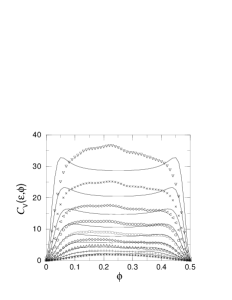
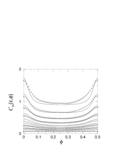
Fig. 1: Velocities and matrix elements in the transition regime between GOE and GUE for the $27\times 27$ Anderson model with $W=1.7$ (symbols), compared to the corresponding semiclassical expressions (lines). The numerical values of $\epsilon$ are $0.158$ ($\bigtriangledown$), $0.224$ ($\times$), $0.316$ ($\lhd$), $0.447$ ($\circ$), $0.631$ ($\Box$), $0.891$ ($\Diamond$), $1.26$ ($\bigtriangleup$), $1.78$ ($+$), $2.51$ ($\ast$).

The numerical data were obtained by averaging over 69 realisations of disorder in the $27\times 27$ Anderson model with $W=1.7$ and over all states in the energy interval $[-3.4,-1.9]$. The two-dimensional case was considered in order to be able to obtain a good numerical accuracy at each flux value in a tolerable computing time. In general we observe good agreement. For a more detailed discussion of the results see [9].

In Fig. 2(a) we show corresponding results for the distribution function of wave-function amplitudes which is defined as follows

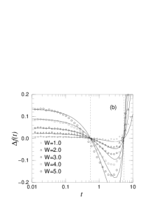
Fig. 2: Wave-function statistics in the $13\times 13\times 13$ Anderson model. (a) GOE to GUE transition of the distribution function in the metallic regime. The Porter-Thomas distributions are shown as dashed lines. The predictions of [10] are show as solid lines. (b) Deviations $\Delta f(t)$ from the Porter–Thomas distribution for the orthogonal case, and several values of disorder strength, $W=1,2,3,4$ and $5$. The results are averaged over the energy interval $[-1.7,-1.4]$. The dashed vertical lines denote the zeros of the first order correction term in Eq. (8). The solid lines are fits according to Eq. (8).

$$f(t)=\Delta\left\langle\sum_{\alpha}\delta(t-|\psi_{\alpha}({\bf r})|^{2}N)\,\delta(E-E_{\alpha})\right\rangle\,.$$ (5)

Within RMT one obtains for $f(t)$ in the limiting cases of GOE and GUE

$$f_{\mathrm{P}T}^{\rm GOE}(t) = {1\over\sqrt{2\pi t}}\exp(-t/2)\,,$$ (6)

$$f_{\mathrm{P}T}^{\rm GUE}(t) = \exp(-t)$$ (7)

(Porter–Thomas distributions [3]). An expression in the transition region between GOE and GUE was derived in [10]. We have computed $f(t)$ numerically for several values of $\phi$ in the $13\times 13\times 13$ Anderson model at $W=0.5$ (in the metallic regime). Our results are shown in Fig. 2(a), where we have plotted $2\sqrt{t}f(t)$ versus $\sqrt{t}$. The results are in good agreement with the analytical formulae (6), (7) and those given in [10].

It was predicted in [6] that the distribution of velocities ceases to be Gaussian in the transition regime between GOE and GUE. The deviations are small, however, and we have not been able to reduce the statistical errors of our numerical results to an extent that a meaningful comparison with the results of [6] becomes possible.

4 Deviations from RMT

Within the non-linear sigma model it is possible to derive $g^{-1}$–corrections to RMT. For distributions of wave-function amplitudes this was done in [13], where in the orthogonal case one obtains

$$f(t)=f^{\rm GOE}_{\mathrm{P}T}(t)\left[1+a_{d}g^{-1}\left(3/2-3t+t^{2}/2\right)+{\cal O}\left(g^{-2}\right)\right]\,.$$ (8)

In the case discussed in Ref. [13], $a_{3}\sim L/l$ where $L$ is the linear dimension of the system and $l$ is the mean free path. Eq. (8) is valid provided $t\ll\sqrt{g/a_{d}}$.

We have performed numerical simulations in the $d=3$ Anderson model, using different values of disorder, and have computed the distribution $f(t)$ by averaging over 400 realizations of disorder. The deviations from the Porter–Thomas distribution, $\Delta f(t)=f(t)/f^{\rm GOE}_{\mathrm{P}T}(t)-1$, is shown in Fig. 2(b). In all cases, the deviations exhibit a characteristic form: the probability of finding small and large amplitudes is enhanced, while the distribution function is reduced near its maximum. We find that $\Delta f(t)$ can be fitted using Eq. (8). At increasingly large disorder, deviations occur at lower values of $t$. In all cases, however, the zeroes of Eq. (8) are well reproduced. Since at weak disorder $l\sim W^{-2}$ one might expect $a_{3}/g\sim W^{4}$. In the present case, however, we find $a_{3}/g\sim W^{2}$. In order to resolve this discrepancy, more accurate numerical data at small values of $W$ are needed. Corresponding results have been obtained for the unitary case.

5 Conclusions

We have analyzed RMT fluctuations of matrix elements and level velocities in the $d=2$ dimensional Anderson model, in the transition regime between GOE and GUE and have found good agreement between the predictions of RMT and our numerical results. For the distribution of wave-function amplitudes in $d=3$ we have studied deviations from RMT, in the form of $g^{-1}$–corrections, as suggested in [13]. Our numerical results can be fitted by the expressions derived in [13], the dependence of the fit parameter $a_{3}$ on $W$ however, differs from what might be expected. In this context it will be very interesting to determine the tails of the distribution functions and compare with the predictions in [12, 14] and [15].
Financial support by the DFG through Sonderforschungsbereich 393 is gratefully acknowledged. V.U. thanks the DAAD for the financial support.

References

- [1] M. L. Mehta Random Matrices and the Statistical Theory of Energy Levels, Academic Press, New York 1991
- [2] K. B. Efetov, Supersymmetry in Disorder and Chaos, Cambridge University Press, Cambridge 1997
- [3] C. E. Porter, in: Statistical Theories of Spectra, ed: C. E. Porter, Academic Press, New York, 1965
- [4] M. Wilkinson, J. Phys. A: Math. Gen. 20 (1987) 4215
- [5] B. Mehlig, N. Taniguchi, unpublished
- [6] N. Taniguchi, A. Hashimoto, B. D. Simons and B. L. Altshuler, Europhys. Lett. 27 (1994) 335
- [7] T.O. de Carvalho, J.P. Keating and J.M. Robbins, J. Phys. A 31 (1998) 5631
- [8] D. Braun and G. Montambaux, Phys. Rev. B 50 (1994) 7776
- [9] V. Uski, R. A. Römer, B. Mehlig and M. Schreiber, unpublished
- [10] V. I. Fal’ko and K. B. Efetov, Phys. Rev. B 50 (1994) 11627
- [11] A. D. Mirlin and Y. V. Fyodorov, J. Phys. A: Math. Gen. 26 (1993) L551
- [12] V. I. Fal’ko and K. B. Efetov, Europhys. Lett. (1995)
- [13] Y. V. Fyodorov and A. D. Mirlin, Phys. Rev. B 51 (1995) 13493
- [14] V. I. Fal’ko and K. B. Efetov, Phys. Rev. B 52 (1995) 17413
- [15] I. E. Smolyarenko and B. L. Altshuler, Phys. Rev. B 55 (1997) 10451
- [16] P. W. Anderson, Phys. Rev. 109 (1958) 1492
- [17] J. Cullum and R. A. Willoughby, Lanczos Algorithms for Large Symmetric Eigenvalue Computations, Birkhäuser, Boston (1985)
- [18] It is assumed that the observable does not commute with the Hamiltonian and has a well-defined classical limit
- [19] The condition ensures that only periodic orbits with periods contribute, so that the diagonal approximation is valid