HIGH TEMPERATURE RELAXATIONAL DYNAMICS
IN
LOW-DIMENSIONAL QUANTUM FIELD THEORIES

Abstract

This paper presents a unified perspective on the results of two recent works (C. Buragohain and S. Sachdev cond-mat/9811083 and S. Sachdev cond-mat/9810399) along with additional background. We describe the low frequency, non-zero temperature, order parameter relaxational dynamics of a number of systems in the vicinity of a quantum critical point. The dynamical correlations are properties of the high temperature limit of renormalizable quantum field theories in spatial dimensions $d=1,2$. We study, as a function of $d$ and the number of order parameter components, $n$, the crossover from the finite frequency, “amplitude fluctuation”, gapped quasiparticle mode in the quantum paramagnet (or Mott insulator), to the zero frequency “phase” ($n\geq 2$) or “domain wall” ($n=1$) relaxation mode near the ordered phase. Implications for dynamic measurements on the high temperature superconductors and antiferromagnetic spin chains are noted.

1 Introduction

Recent neutron scattering experiments by Aeppli et al.[1] have studied the two-dimensional incommensurate spin correlations in the normal state of the high temperature superconductor ${\rm La}_{x}{\rm Sr}_{1-x}{\rm CuO}_{4}$ at $x\approx 0.15$ in some detail. In particular, they have determined the scattering cross section over a significant portion of the wavevector, frequency and temperature space. One of their striking observations has been that, while the dynamic structure factor of the electronic spins has quite an intricate functional form over this three-dimensional parameter space, the results become quite simple and explicable when interpreted in terms of the non-zero temperature dynamical properties of a system in the vicinity of a quantum critical point [2, 3]. The data are consistent with such an interpretation over a decade in temperature and in over two decades of the peak scattering amplitude, and indicate that there is a nearby quantum critical point with dynamic critical exponent $z\approx 1$. The nature of the measured spin correlations indicates that this quantum critical point is the position of a quantum phase transition to an insulating, charge- and spin-ordered ground state. Varying the doping concentration, $x$, alone is not expected to be sufficient to access this ordered state, and authors [1] asserted that a second tuning parameter (‘$y$’) is necessary; e.g. it is known that replacing some of the ${\rm Sr}$ by ${\rm Nd}$ allows one to move along the $y$ axis [4].

In this paper, we will review recent theoretical work studying non-zero temperature ($T$) dynamical response functions closely related to those measured in the neutron scattering experiment of Aeppli et al. [1] We will examine a simple class of models in spatial dimension $d=1,2$, which exhibit quantum ordering transitions with $z=1$. All of the models we shall study are closely related to the following quantum field theory of a real, $n$-component, scalar field $\phi_{\alpha}$ ($\alpha=1\ldots n$):

$${\cal Z}_{Q}=\int{\cal D}\phi_{\alpha}(x,\tau)\exp\left(-\int d^{d}x\int_{0}^{1/T}d\tau\,{\cal L}_{Q}\right)$$

$${\cal L}_{Q}=\frac{1}{2}\left[\frac{1}{c^{2}}(\partial_{\tau}\phi_{\alpha})^{2}+(\nabla_{x}\phi_{\alpha})^{2}+(r_{c}+r)\phi_{\alpha}^{2}\right]+\frac{u}{4!}\left(\phi_{\alpha}^{2}\right)^{2}.$$ (1)

Here we are using units with $\hbar=k_{B}=1$, $x$ is the $d$-dimensional spatial co-ordinate, $\tau$ is imaginary time, $c$ is a velocity, and $r_{c}$, $r$ and $u$ are coupling constants. The co-efficient of the $\phi_{\alpha}^{2}$ term (the ‘mass’ term) has been written as $r+r_{c}$ for convenience. The quartic non-linearity $u$ makes ${\cal Z}_{Q}$ as interacting quantum field theory, and it ultimately responsible for the dynamic relaxation phenomena we shall describe. For appropriate values of $d$ and $n$, the model ${\cal Z}_{Q}$ exhibits a $T=0$ quantum transition between an ordered phase with $\langle\phi_{\alpha}\rangle\neq 0$, and a quantum paramagnet with complete ${\rm O}(n)$ symmetry; the value of $r_{c}$ is chosen so that this transition occurs at $r=0$. In physical applications of ${\cal Z}_{Q}$, the case $n=1$ describes the Ising model in a transverse field, the case $n=2$ case describes a superfluid-insulator transition (with $\phi_{1}+i\phi_{2}$, the complex superfluid order parameter), and $n=3$ describes spin fluctuations in a collinear quantum antiferromagnet (with $\phi_{\alpha}$ the antiferromagnetic order parameter).

We will be interested in the real-time dynamic properties of ${\cal Z}_{Q}$ in the high $T$ limit of the continuum quantum field theory (in some cases, this is also the ‘quantum critical’ region [5]). More specifically, in the vicinity of a quantum critical point, the theory ${\cal Z}_{Q}$ can be characterized by two distinct energy scales. The first, is a low energy scale, characterizing the deviation from the system from the quantum critical point at $r=0$: this varies as $b|r|^{z\nu}$, where $\nu$ is the correlation length exponent, and $b$ is a non-universal, cutoff-dependent constant needed to make the expression have physical units of energy; this low energy scale is the central quantity characterizing the continuum quantum field theory. The second, is a high energy scale, and is of order $c\Lambda$, where $\Lambda$ is a high-momentum cutoff needed at intermediate stages to define the continuum limit of ${\cal Z}_{Q}$; this energy scale plays no role in the continuum quantum field theory. We will be assuming here that the temperature is in between these two energy scales i.e.

$$b|r|^{z\nu}\ll T\ll c\Lambda.$$ (2)

We will characterize the response of the system by the dynamic susceptibility, $\chi(k,\omega_{n})$, defined by

$$\chi(k,\omega_{n})\equiv\frac{1}{n}\int_{0}^{1/T}d\tau\int d^{d}x\,\sum_{\alpha=1}^{n}\langle\phi_{\alpha}(x,\tau)\phi_{\alpha}(0,0)\rangle e^{-i(kx-\omega_{n}\tau)},$$ (3)

where $k$ is the wavevector, $\omega_{n}$ the imaginary frequency; throughout we will use the symbol $\omega_{n}$ to refer to imaginary frequencies, while the use of $\omega$ will imply the expression has been analytically continued to real frequencies. Further, the static susceptibility, $\chi(k)$, is defined by

$$\chi(k)\equiv\chi(k,\omega_{n}=0).$$ (4)

We shall be especially interested here in a relaxation function ${\cal R}(k,\omega)$, which we define as

$${\cal R}(k,\omega)=\frac{1}{\chi(k)}\frac{2}{\omega}\mbox{Im}\chi(k,\omega).$$ (5)

This is an even function of $\omega$ with the dimensions of time, and the Kramers-Kronig relation implies that

$$\int_{-\infty}^{\infty}\frac{d\omega}{2\pi}\,{\cal R}(k,\omega)=1.$$ (6)

After a Fourier transform to real time, ${\cal R}(k,t)$ (with ${\cal R}(k,t=0)=1$) describes the time-dependent relaxation of spin correlations at wavevector $k$ due to quantum and thermal fluctuations.

(In a regime where the predominant fluctuations have an energy much smaller than $T$, the low frequency dynamics becomes effectively classical, and then the fluctuation-dissipation theorem implies that

$${\cal R}(k,\omega)\approx\frac{S(k,\omega)}{S(k)},$$ (7)

where $S(k,\omega)$ is the dynamic structure factor, and $S(k)$ is the equal-time structure factor. However, this relationship is not generally true for a quantum system, and for clarity, we will always use (5) as our defining relation.)

The following sections will describe the behavior of ${\cal R}(k,\omega)$ in the high $T$ limit of the continuum quantum theory ${\cal Z}_{Q}$ for various physically interesting cases in low dimensions: we will consider the case $n=1$, $d=1$ in Section 2, the case $n=3$, $d=1$ in Section 3, and all values of $n$ in $d=2$ in Section 4.

2 Ising chain in a transverse field

The Ising chain in a transverse field has the Hamiltonian

$$H_{I}=-J\sum_{i}\left(g\hat{\sigma}^{x}_{i}+\hat{\sigma}^{z}_{i}\hat{\sigma}^{z}_{i+1}\right),$$ (8)

where $\hat{\sigma}^{x,z}_{i}$ are Pauli matrices on the sites, $i$, of a $d=1$ chain with lattice spacing $a$. This model has a quantum critical point at $g=1$, whose vicinity is believed to be described by the $d=1$, $n=1$ case of ${\cal Z}_{Q}$. Under this mapping, the field-theoretic correlators of $\phi_{\alpha}$ under ${\cal Z}_{Q}$ are equivalent to the long-distance, long-time correlators of the order parameter $\hat{\sigma}^{z}$ under the lattice model $H_{I}$.

The continuum high $T$ dynamical response of (8) can be computed exactly by a special trick relying on the conformal invariance of the critical theory at $g=1$ [6]. The result for $\chi(k,\omega)$ is

$$\chi(k,\omega)=\frac{Zc}{T^{7/4}}\frac{G_{I}(0)}{4\pi}\frac{\Gamma(7/8)}{\Gamma(1/8)}\frac{\displaystyle\Gamma\left(\frac{1}{16}-i\frac{\omega+ck}{4\pi T}\right)\Gamma\left(\frac{1}{16}-i\frac{\omega-ck}{4\pi T}\right)}{\displaystyle\Gamma\left(\frac{15}{16}-i\frac{\omega+ck}{4\pi T}\right)\Gamma\left(\frac{15}{16}-i\frac{\omega-ck}{4\pi T}\right)}.$$ (9)

Here $Z=J^{-1/4}$, $c=2Ja$, and $G_{I}(0)=0.858715\ldots$. We show a plot of $\mbox{Im}\chi$ in Fig 1.

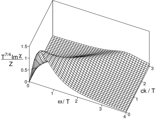
Figure 1: High temperature dynamic susceptibility, $T^{7/4}\mbox{Im}\chi(k,\omega)/Z$ in (9) of the quantum Ising chain ($d=1$, $n=1$) as a function of $\omega/T$ and $ck/T$.

For $\omega,ck\gg T$ there is a well-defined ‘reactive’ peak in $\mbox{Im}\chi$ at $\omega\approx ck$ reflecting the excitations of the $T=0$ quantum critical point, which have an energy threshhold at $\omega=ck$. However the low frequency dynamics is quite different, and for $\omega,ck\ll T$ we cross-over to the quantum relaxational regime [3]. This is made clear by an examination of $\mbox{Im}\chi(k,\omega)/\omega$ as a function of $\omega/T$ and $ck/T$, which is shown in Fig 2.

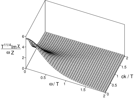
Figure 2: Plot of the spectral density of the quantum Ising chain ($d=1$, $n=1$) $T^{11/4}\mbox{Im}\chi(k,\omega)/\omega Z$ as a function of $\omega/T$ and $ck/T$. Note that this is simply the quantity in Fig 1 divided by $\omega$. The reactive peaks at $\omega\approx ck$ in Fig 1 are essentially invisible, and the plot is dominated by a large relaxational peak at zero wavevector and frequency.

Now the reactive peaks at $\omega\sim ck$ are just about invisible, and the spectral density is dominated by a large relaxational peak at zero frequency. We can understand the structure of Fig 2 by expanding the inverse of (9) in powers of $k$ and $\omega$; this expansion has the form

$$\chi(k,\omega)=\frac{\chi(0)}{1-i(\omega/\omega_{1})+k^{2}\widetilde{\xi}^{2}-(\omega/\omega_{2})^{2}},$$ (10)

where $\chi(0)\sim T^{-7/4}$, and $\omega_{1,2}$ and $\widetilde{\xi}$ are parameters characterizing the expansion. For $k$ not too large, the $\omega$ dependence in (10) is simply the response of a strongly damped harmonic oscillator: this is the reason we have identified the low frequency dynamics as “relaxational”. The function in (10) provides an excellent description of the spectral response in Fig 2. We determined the best fit values of the parameters $\omega_{1,2}$ and $\widetilde{\xi}$ by minimizing the mean square difference between the values of $\mbox{Im}\chi(k,\omega)/\omega$ given by (10) and (9) over the range $0<\omega<2T$ and $0<ck<2T$ and obtained

$$\omega_{1} = 0.396~{}T$$

$$\omega_{2} = 0.795~{}T$$

$$\widetilde{\xi} = 1.280~{}c/T.$$ (11)

The quality of the fit is shown in Figs 3 and 4. In Fig 3 we compare the predictions of (9) and (10) for $\mbox{Im}\chi(k,\omega)/\omega$ at $\omega=0$ as a function of $ck/T$. The form (10) predicts a Lorentzian-squared response function and this is seen to provide a better fit than a Lorentzian—a similar Lorentzian-squared response was used in analyzing the data in Ref. 1. In Fig 4 we plot the predictions of (9) and (10) for ${\cal R}(k,\omega)$ at $ck/T=0,1.5$ as a function of $\omega/T$.

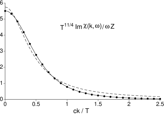
Figure 3: Comparison of the predictions of (9) (dots) and (10) (solid line) for $\mbox{Im}\chi(k,\omega)/\omega$ of the quantum Ising chain ($d=1$, $n=1$) at $\omega=0$ as a function of $ck/T$. The best fit parameters in (11) were used. The function (10) yields the square of a Lorentzian as a function of $k$; a best fit by just a Lorentzian is also shown (dashed line), and is much poorer.

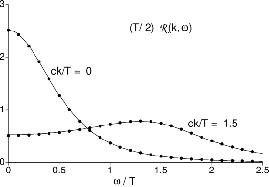
Figure 4: Comparison of the predictions of (9) (dots) and (10) (solid line) for the relaxation function $(T/2){\cal R}(k,\omega)$ of the quantum Ising chain ($d=1$, $n=1$) as a function of $\omega/T$ at $ck/T=0,1.5$.

For $k=0$ ($\omega=0$) there is a large overdamped peak at $\omega=0$ ($k=0$), but a weak reactive peak at $\omega\sim ck$ does make an appearance at larger wavevectors or frequencies.

For an alternative, and more precise, characterization of the relaxational dynamics we can introduce the relaxation rate $\Gamma_{R}$ defined by

$$\Gamma_{R}^{-1}\equiv\frac{{\cal R}(0,0)}{2};$$ (12)

we have chosen this definition because for the suggestive functional form (10), $\Gamma_{R}=\omega_{1}$, the frequency characterizing the damping. However, using (9) we determine:

$$\Gamma_{R} = \left(2\tan\frac{\pi}{16}\right)\frac{k_{B}T}{\hbar}$$ (13)

$$\approx 0.397825\frac{k_{B}T}{\hbar},$$

where we have inserted physical units to emphasize the universality of the result.

An important property of the present high $T$ dynamical results is that at the scale of the characteristic rate $\Gamma_{R}$, the dynamics of the system involves intrinsic quantum effects which cannot be neglected. Description by an effective classical model would require that $\Gamma_{R}\ll k_{B}T/\hbar$, which is thus not satisfied here.

To obtain an intuitive physical picture of the above quantum relaxational dynamics, it is useful to consider approaching the high $T$ limit by gradually rising the temperature (while keeping all other couplings fixed) from the low $T$ limit where $T\ll b|r|^{z\nu}$.

First, consider the low $T$ limit on the magnetically ordered side. Here the excitations above the ground state are ‘domain walls’ which separate regions in which the Ising order parameter has opposite signs. These domain walls can move easily without significant change of energy, and their low energy motion leads to a large relaxational peak in ${\cal R}(k,\omega)$ at $\omega=0$, $k=0$ [7]. At very low $T$, the domain walls are very dilute, and their spacing is much larger than their thermal de Broglie wavelengths—consequently their motion can be described in a classical model. However, as $T$ is raised into the high $T$ regime, their spacing becomes of order their de Broglie wavelength, and the relaxation rate of their collisional dynamics becomes of order $T$: this is leads to the relaxational peak in Fig 4.

Second, we can begin by considering the low $T$ limit on the quantum paramagnetic side. Now the excitations are local ‘flipped spins’ which require a finite energy, $\Delta$, to create them. So there is a sharp peak in ${\cal R}(k,\omega)$ at $\omega=\Delta$, which is broadened by collisions with the dilute, classical gas of pre-existing quasiparticles. In the language of the field $\phi_{\alpha}$, this finite frequency peak arises from amplitude fluctuations in $\phi$ about a local minimum in its effective potential. As $T$ is raised, the quasiparticle gas becomes dense with the mean-particle spacing becoming of order their de Broglie wavelength, the quasiparticle line-width becomes of order $T$, and the peak in ${\cal R}(k,\omega)$ eventually moves to $\omega=0$.

3 Gapped, Heisenberg antiferromagnetic chains

In this section we will consider ${\cal Z}_{Q}$ for the case $d=1$, $n=3$, which describes the low energy fluctuations of certain one-dimensional quantum antiferromagnets: chains of integer spin $S$, or $p$-leg ladders with $p$ even. The ground state of these systems is always a quantum paramagnet with an energy gap, $\Delta$, and there is no magnetically ordered state. So strictly speaking, there is no quantum critical point, and it may appear that the general arguments of Section 1 do not apply. However, it is still possible to define a universal, continuum high $T$ limit of the quantum theory. We have to replace the condition (2) by

$$\Delta\ll T\ll c\Lambda\sim J,$$ (14)

where $J$ is a typical exchange constant of the antiferromagnet, but, unlike (2), the energy gap, $\Delta$, is always non-zero. So we have to pick a system with $\Delta$ much smaller than any microscopic energy scale. As $\Delta$ becomes exponentially small as $S$ (or $p$) is increased, this is quite easily achieved. In a formal sense, we can consider the following an analysis of the high $T$ dynamics of the ‘quantum’ critical point reached in the limit $S\rightarrow\infty$, when $\Delta$ becomes vanishingly small.

The high $T$ limit introduced above has been analyzed in some detail in two recent papers [8, 9]. It was argued that there is an effective classical non-linear wave problem that describes the long time relaxation dynamics. The degrees of freedom of this classical model are a 3-component unit length field ${\bf n}(x,t)$, ${\bf n}^{2}=1$, which describes the local orientation of the antiferromagnetic order parameter, and its canonically conjugate angular momentum, ${\bf L}(x,t)$, which measures the ferromagnetic component of the local spin density. The equal time correlations of ${\bf L}$ and ${\bf n}$ are described by the following continuum classical partition function

$${\cal Z}_{1C}=\int{\cal D}{\bf n}(x){\cal D}{\bf L}(x)\delta({\bf n}^{2}-1)\delta({\bf L}\cdot{\bf n})\exp\left(-\frac{{\cal H}_{1C}}{T}\right)$$

$${\cal H}_{1C}=\frac{1}{2}\int dx\,\left[T\xi\left(\frac{d{\bf n}}{dx}\right)^{2}+\frac{1}{\chi_{u\perp}}{\bf L}^{2}\right].$$ (15)

The parameters in this partition function are determined universally in terms of $\Delta$, $T$, and $c$, and exact expressions are known in the limit (14) [8, 9]. The correlation length, $\xi$, is given by

$$\xi=\frac{c}{2\pi T}\ln\left(\frac{32\pi e^{-(1+\gamma)}T}{\Delta}\right),$$ (16)

where $\gamma$ is Euler’s constant. The quantity $\chi_{u\perp}$ is the susceptibility to a uniform magnetic field (which couples to the ferromagnetic moment) in a direction orthogonal to the local antiferromagnetic order; it is related to the rotationally averaged uniform susceptibility, $\chi_{u}$, by

$$\chi_{u}=\frac{2}{3}\chi_{u\perp},$$ (17)

and $\chi_{u}$ is given by

$$\chi_{u}=\frac{1}{3\pi c}\ln\left(\frac{32\pi e^{-(2+\gamma)}T}{\Delta}\right).$$ (18)

As we will see below, with these parameters in hand, the characteristic excitation of the classical model (15) has energy $\varepsilon\sim T/\ln(T/\Delta)$. For $T\gg\Delta$, this is parametrically smaller than $T$. So the occupation number of the wave modes with energy $\varepsilon$ will be much larger than unity, and the quantum Bose function will take the classical equipartition value $T/\varepsilon$. This is the argument which justifies use of a classical model in this high $T$ limit.

All equal time correlations of the model (15) can be computed exactly. As this is a model to which the classical fluctuation-dissipation theorem applies, the equal time, two-point ${\bf n}$ correlator is directly related to the static susceptibility; the underlying quantum fluctuations however do induce an overall wavefunction renormalization factor [8, 9]. The two point ${\bf n}$ correlator decays exponentially on the scale $\xi$, and by its Fourier transform to momentum space we obtain

$$T\chi(k)={\cal A}\left[\ln\left(\frac{T}{\Delta}\right)\right]^{2}\frac{2\xi/3}{(1+k^{2}\xi^{2})}.$$ (19)

Here ${\cal A}$ is a non-universal amplitude which determines the scale of the field $\phi_{\alpha}$, and the multiplicative logarithmic factor comes from the underlying quantum fluctuations; the remaining is just the Fourier transform of $e^{-|x|/\xi}/3$, the $1/3$ coming from the $1/n$ in (3).

Let us now turn to the unequal time correlations. To obtain these, we have to supplement ${\cal Z}_{1C}$ with equations of motion, which have been argued [8, 9] to be the Hamilton-Jacobi equations associated with the Poisson brackets of ${\bf n}$ and its canonically conjugate angular momentum ${\bf L}$:

$$\left\{L_{\alpha}(x),L_{\beta}(x^{\prime})\right\}_{PB} = \epsilon_{\alpha\beta\gamma}L_{\gamma}(x)\delta(x-x^{\prime})$$

$$\left\{L_{\alpha}(x),n_{\beta}(x^{\prime})\right\}_{PB} = \epsilon_{\alpha\beta\gamma}n_{\gamma}(x)\delta(x-x^{\prime})$$

$$\left\{n_{\alpha}(x),n_{\beta}(x^{\prime})\right\}_{PB} = 0.$$ (20)

From this, and (15), we obtain directly the equations of motion for the quasi-classical waves

$$\frac{\partial{\bf n}}{\partial t} = \{{\bf n},{\cal H}_{1C}\}_{PB}$$

$$= \frac{1}{\chi_{u\perp}}{\bf L}\times{\bf n}$$

$$\frac{\partial{\bf L}}{\partial t} = \{{\bf L},{\cal H}_{1C}\}_{PB}$$ (21)

$$= (T\xi){\bf n}\times\frac{\partial^{2}{\bf n}}{\partial x^{2}}.$$

To compute the needed unequal time correlation functions, pick a set of initial conditions for ${\bf n}(x)$, ${\bf L}(x)$ from the ensemble (15). Evolve these deterministically in time using the equations of motion (21). The value of the correlator is then the product of the appropriate time-dependent fields, averaged over the set of all initial conditions. We also note here that simple analysis of the differential equations (21) shows that small disturbances about a nearly ordered ${\bf n}$ configuration travel with a characteristic velocity $c(T)$ given by

$$c(T)=(T\xi(T)/\chi_{u\perp}(T))^{1/2},$$ (22)

which is a basic relationship between thermodynamic quantities and the velocity $c(T)$. Notice from (16) and (18) that to leading logarithms $c(T)\approx c$, but this result is not satisfied by the subleading terms. The characteristic excitation will have energy $\varepsilon\sim c/\xi$, and this leads to our estimate for $\varepsilon$ made earlier, when we justified the validity of a classical model.

The classical dynamics problem defined by (15) and (21) obeys that the crucial property of being free of all ultraviolet divergences. Consequently, we may determine its characteristic length and time scales by simple engineering dimensional analysis, as no short distance cutoff scale is going to transform into an anomalous dimension. Indeed, a straightforward analysis shows that this classical problem is free of dimensionless parameters, and is a unique, parameter-free theory. This is seen by defining

$$\overline{x} = \frac{x}{\xi}$$

$$\overline{t} = \frac{t}{\tau_{\varphi}}$$

$$\overline{{\bf L}} = {\bf L}\sqrt{\frac{\xi}{T\chi_{u\perp}}},$$ (23)

where the characteristic time, $\tau_{\varphi}$, is given by

$$\tau_{\varphi}=\sqrt{\frac{\xi\chi_{u\perp}}{T}};$$ (24)

our notation suggests that $\tau_{\varphi}$ (like $\Gamma_{R}^{-1}$ earlier) is a phase coherence time beyond which relaxational dynamics of damped spin waves takes over. Inserting (23,24) into (15) and (21), we find that all parameters disappear and the partition function and equations of motion acquire a unique, dimensionless form, given by setting $T=\xi=\chi_{u\perp}=1$ in them.

The above transformations allow us to easily obtain a scaling form for the relaxation function ${\cal R}$:

$${\cal R}(k,\omega)=\tau_{\varphi}\Psi_{{\cal R}}(k\xi,\omega\tau_{\varphi}),$$ (25)

where $\Psi_{{\cal R}}$ is a universal scaling function, normalized as in (6). Further information on the structure of $\Psi_{{\cal R}}$ was obtained [9] by a combination of analytic and numerical methods. At sufficiently large $k\xi$, we expect a pair of broadened, reactive, ‘spin-wave’ peaks at $\omega\approx c(T)k$ (with $c(T)$ given in (22)), which are similar to those found in the high $T$ limit of the quantum Ising chain in Fig 4. For the opposite limit of small $k\xi$, we present numerical results for $\Psi_{{\cal R}}(0,\overline{\omega})$ in Fig 5.

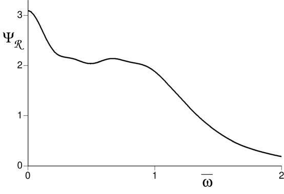
Figure 5: Numerical results [9] for the scaling function, $\Psi_{{\cal R}}(0,\overline{\omega})$, for the relaxation function ${\cal R}$ of the $d=1$, $n=3$ case of ${\cal Z}_{Q}$ appearing in (25). The dimensionless frequency $\overline{\omega}=\omega\tau_{\varphi}$.

There is a sharp relaxational peak at $\overline{\omega}=0$, which is again similar to that found in the high $T$ limit of the quantum Ising chain in Fig 4. However, there is now a well-defined shoulder at $\overline{\omega}\approx 0.7$ which was not found in the Ising case. This shoulder is a remnant of the large $n$ result [3, 10] which predicts a delta function at $\omega\sim T/\ln(T/\Delta)$. So $N=3$ is large enough for this finite frequency oscillation to survive in the high $T$ limit.

There is alternative, helpful way to view this oscillation frequency. The underlying degree of freedom in our dynamical field theory has a fixed amplitude, with $|{\bf n}|=1$. However, correlations of ${\bf n}$ decay exponentially on a length scale $\xi$—so if we imagine coarse-graining out to $\xi$, it is reasonable to expect significant amplitude fluctuations in the coarse-grained field. It is now useful to visualize an effective field $\phi_{\alpha}$ with no length constraint, which is just the field we introduced in Section 1. On a length scale of order $\xi$, we expect the effective potential controlling fluctuations of $\phi_{\alpha}$ to have minimum at a non-zero value of $|\phi_{\alpha}|$, but to also allow fluctuations in $|\phi_{\alpha}|$ about this minimum. The finite frequency in Fig 5 is due to the harmonic oscillations of $\phi_{\alpha}$ about this potential minimum, while the dominant peak at $\omega=0$ is due to angular fluctuations along the zero energy contour in the effective potential. This is interpretation is also consistent with the large $n$ limit, in which we freely integrate over all components of ${\bf n}$, and so angular and amplitude fluctuations are not distinguished. The above argument could also have been applied to the quantum Ising chain (in this case, angular fluctuations are replaced by low-energy domain wall motion), but the absence of such a reactive, finite frequency peak at $k=0$ in Fig 4 indicates that $n=1$ is too far from $n=\infty$ for any remnant of this large $n$ physics to survive.

4 Order parameter dynamics in $d=2$

Determination of the long time dynamics in $d=2$ is a strongly coupled problem and remains unsolved. As in the analysis in Section 2, we expect a phase coherence time, $\tau_{\phi}$, and an inverse relaxation rate, $\Gamma_{R}^{-1}$, of order $T$, and quantum and thermal fluctuations to play an equally important role.

However, it has been argued recently [11], that within the context of an expansion in

$$\epsilon=3-d,$$ (26)

it is possible to separate quantum and thermal effects into two distinct stages of the calculation, and to derive an effective classical wave model for the long time dynamics. As in Section 3, we first derive an effective action for the static susceptibility, and then supplement it with equations of motion to obtain the unequal time correlations. We define the zero Matsubara frequency component of $\phi_{\alpha}$ by

$$\Phi_{\alpha}(x)=T\int_{0}^{1/T}d\tau\,\phi_{\alpha}(x,\tau),$$ (27)

and derive an effective action for $\Phi_{\alpha}$ by integrating out the non-zero Matsubara frequency components of $\phi_{\alpha}$. To leading non-trivial order in an expansion in $\epsilon$, this leads to the following effective action

$${\cal Z}_{2C}=\int{\cal D}\Phi_{\alpha}(x){\cal D}\Pi_{\alpha}(x)\exp\left(-\frac{{\cal H}_{2C}}{T}\right)$$

$${\cal H}_{2C}=\int d^{d}x\,\left\{\frac{1}{2}\left[c^{2}\Pi_{\alpha}^{2}+(\nabla_{x}\Phi_{\alpha})^{2}+\widetilde{R}\,\Phi_{\alpha}^{2}\right]+\frac{U}{4!}\left(\Phi_{\alpha}^{2}\right)^{2}\right\}.$$ (28)

As in (15), along with the functional integral over $\Phi_{\alpha}(x)$, we have included an integral over a conjugate momentum field $\Pi_{\alpha}(x)$ which will be important for our subsequent treatment of the dynamics; for now it easy to see that the Gaussian integral over $\Pi_{\alpha}$ can be performed exactly, and it leaves the correlations of $\Phi_{\alpha}$ under ${\cal Z}_{2C}$ unchanged. The coupling constants in (28) are universally related to the underlying field theory ${\cal Z}_{Q}$ controlling the quantum critical point. Before specifying these, it is crucial to understand the nature of the ultraviolet divergences in ${\cal Z}_{2C}$ considered as a classical field theory in its own right. From standard field-theoretic analyses [12] it is known that ${\cal Z}_{2C}$ has only one ultraviolet divergence, coming from a single one-loop tadpole graph in the self energy: consequently, by trading the bare ‘mass’ $\widetilde{R}$ for a renormalized mass $R$ defined by

$$\widetilde{R}=R-TU\left(\frac{n+2}{6}\right)\int^{\Lambda}\frac{d^{d}k}{(2\pi)^{d}}\frac{1}{k^{2}+R},$$ (29)

we can remove all cutoff dependencies in the correlators of ${\cal Z}_{2C}$ (there are some additional divergences, associated with composite operators, which appear when two or more field operators approach each other in space: we will not be concerned with these here). All observables of ${\cal Z}_{2C}$ are then universal functions of the couplings $R$ and $U$. Moreover, it is precisely these couplings that are universally computed from the underlying quantum field theory ${\cal Z}_{Q}$. Actually, instead to dealing with $R$ and $U$ as the two independent parameters controlling correlators of ${\cal Z}_{2C}$, it is convenient to replace $U$ by the dimensionless parameter ${\cal G}$ defined by

$${\cal G}\equiv\frac{TU}{R^{(4-d)/2}},$$ (30)

which is analogous to the Ginzburg parameter. In the high $T$ limit (2), these parameters were shown to have the following [13, 11] universal values to leading order in $\epsilon$

$$R = \epsilon\left(\frac{n+2}{n+8}\right)\frac{2\pi^{2}(T/c)^{2}}{3}$$

$${\cal G} = \sqrt{\epsilon}\frac{48\pi\sqrt{3}}{\sqrt{2(n+2)(n+8)}}.$$ (31)

As one lowers the temperature from the continuum high $T$ limit, both $R$ and ${\cal G}$ vary as universal functions of $r/T^{1/(z\nu)}$: $R$ decreases and ${\cal G}$ increases as we lower the temperature into the magnetically ordered region ($r<0$), while $R$ increases and ${\cal G}$ decreases as we lower the temperature into the quantum paramagnetic region ($r>0$).

The values in (31) are the key to the argument justifying the use of a classical dynamical model for small $\epsilon$. From (28) it is clear that the characteristic $\Phi_{\alpha}$ fluctuations have an energy of order $c\sqrt{R}\sim\sqrt{\epsilon}T$. As in Section 3, this energy is parametrically smaller than $T$, and so the occupation number of the relevant $\Phi_{\alpha}$ will be given by their classical equipartition value. This also means that the classical fluctuation dissipation theorem is obeyed, and the static susceptibility, $\chi(k)$, computed from (28) by

$$T\chi(k)=\frac{1}{n}\sum_{\alpha=1}^{n}\langle|\Phi_{\alpha}(k)|^{2}\rangle,$$ (32)

is also the equal-time correlation of $\phi_{\alpha}$.

We can now specify the recipe to compute the unequal time correlations of $\phi_{\alpha}$, in manner which parallels Section 3. The fundamental Poisson bracket is

$$\{\Phi_{\alpha}(x),\Pi_{\beta}(x^{\prime})\}_{PB}=\delta_{\alpha\beta}\delta(x-x^{\prime}),$$ (33)

and the Hamiltonian ${\cal H}_{2C}$ then leads to the Hamilton-Jacobi equations of motion

$$\frac{\partial\Phi_{\alpha}}{\partial t} = \left\{\Phi_{\alpha}(x),{\cal H}_{2C}\right\}_{PB}$$ (34)

$$= c^{2}\Pi_{\alpha},$$

and

$$\frac{\partial\Pi_{\alpha}}{\partial t} = \left\{\Pi_{\alpha}(x),{\cal H}_{2C}\right\}_{PB}$$ (35)

$$= \nabla_{x}^{2}\Phi_{\alpha}-\widetilde{R}\Phi_{\alpha}-\frac{U}{6}(\Phi_{\beta}^{2})\Phi_{\alpha},$$

The equations (28), (34) and (35) define the central dynamical non-linear wave model of this section. We will compute correlations of the field $\Phi_{\alpha}$ at unequal times, averaged over the set of initial conditions specified by (28). Notice all the thermal ‘noise’ arises only in the random set of initial conditions. The subsequent time evolution is then completely deterministic, and precisely conserves energy, momentum, and total ${\rm O}(n)$ charge. This should be contrasted with the classical dynamical models studied in the theory of dynamic critical phenomena [14, 15], where there are explicit damping co-efficients, along with statistical noise terms, in the equations of motion.

The dynamical model has been defined above in the continuum, and so we need to consider the nature of its short distance singularities. As in Section 3, we assert [11] that the only short distance singularities are those already present in the equal time correlations analyzed earlier. These were removed by the simple renormalization in (29), which is therefore adequate also for the unequal time correlations. With this knowledge in hand, we can immediately write down the universal scaling form obeyed by the relaxation function by simple arguments based upon analysis of engineering dimensions. The analog of (25) is now

$${\cal R}(k,\omega)=\frac{1}{c\sqrt{R}}\Psi_{{\cal R}}\left(\frac{k}{\sqrt{R}},\frac{\omega}{c\sqrt{R}},{\cal G}\right),$$ (36)

where $\Psi_{{\cal R}}$ is a universal function we wish to determine.

It now remains to solve the dynamical problem specified by (28), (34) and (35), and so determine $\Psi_{{\cal R}}$. For small $\epsilon$, the dimensionless strength of the non-linearity ${\cal G}$ in (31) is small; nevertheless we cannot use perturbation theory in ${\cal G}$, because this fails in the low frequency limit. In other words, the dynamical problem remains strongly coupled even for small $\epsilon$.

The only remaining possibility is to numerically solve the strong-coupling dynamical problem. Formally, we are carrying out an $\epsilon$ expansion, and so the numerical solution should be obtained for $d$ just below 3. However, it is naturally much simpler to simulate directly in $d=2$, which is also the dimensionality of physical interest. Therefore, the approach to the solution of the dynamic problem in the quantum critical region breaks down into two systematic steps: (i) Use the $\epsilon=3-d$ expansion to derive an effective classical non-linear wave problem [13] characterized by the couplings $R$ and ${\cal G}$. (ii) Obtain the exact numerical solution [11] of the classical non-linear wave problem at these values of $R$ and ${\cal G}$ directly in $d=2$. This division of the problem into two rather disjointed steps is also physically reasonable: it is primarily for the classical thermal fluctuations that the dimensionality $d=2$ plays a special role, and the cases $n=1,2$ (which have non-zero temperature phase transitions above the magnetically ordered phase) and $n\geq 3$ (which do not have a non-zero temperature phase transition) are strongly distinguished—so it is important to treat these exactly; on the other hand, the $\epsilon=3-d$ expansion provides a reasonable treatment of the quantum fluctuations down to $d=2$ for all $n$.

Figs 6–8 contain the results of a recent numerical computation of the scaling function in (36) at $k=0$.

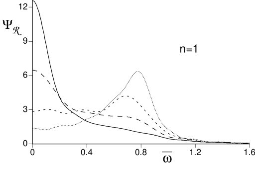
Figure 6: Numerical results [11] for the zero momentum scaling function $\Psi_{{\cal R}}(0,\overline{\omega},{\cal G})$ for the relaxation function, ${\cal R}$, appearing in (36) for the $d=2$, $n=1$ model ${\cal Z}_{Q}$. The dimensionless frequency $\overline{\omega}=\omega/c\sqrt{R}$. Results are shown for ${\cal G}=25$ (dots), ${\cal G}=30$ (short dashes), ${\cal G}=35$ (long dashes) and ${\cal G}=40$ (full line). The high $T$ limit value of ${\cal G}$ in (31) evaluates to ${\cal G}=35.5$ at $\epsilon=1$ and $n=1$.

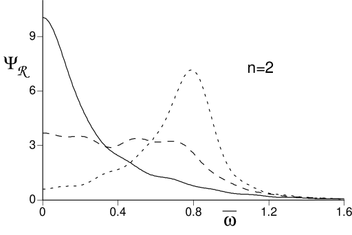
Figure 7: As in Fig 6 but for $d=2$, $n=2$. The values of ${\cal G}$ are now ${\cal G}=20$ (short dashes), ${\cal G}=30$ (long dashes) and ${\cal G}=40$ (full line). The high $T$ limit value of ${\cal G}$ in (31) evaluates to ${\cal G}=29.2$ at $\epsilon=1$ and $n=2$.

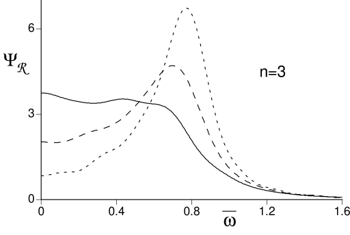
Figure 8: As in Fig 6 but for $d=2$, $n=3$. The values of ${\cal G}$ are now ${\cal G}=20$ (short dashes), ${\cal G}=25$ (long dashes) and ${\cal G}=30$ (full line). The high $T$ limit value of ${\cal G}$ in (31) evaluates to ${\cal G}=24.9$ at $\epsilon=1$ and $n=3$.

These results are the analog of Fig 4 for the Ising chain and Fig 5 for the $d=1$, $n=3$ case. They show a consistent trend from small values of ${\cal G}$ and large values of $n$ to large values of ${\cal G}$ and small values of $n$, and we discuss the physical interpretation of the two limiting cases in turn.

For smaller ${\cal G}$ and larger $n$, we observe a peak in ${\cal R}(0,\omega)$ at a non-zero frequency. This peak is the remnant of a delta function obtained in the large $n$ limit at a frequency $\omega\sim T$. In the present computation, it is clear that the peak is due to amplitude fluctuations as $\Phi_{\alpha}$ oscillates about the minimum in its effective potential at $\Phi_{\alpha}=0$. As ${\cal G}$ is reduced, we move out of the high $T$ region into the low $T$ region above the quantum paramagnet, and this finite frequency, amplitude fluctuation peak connects smoothly with the quantum paramagnetic quasiparticle peak. Of course, once we are in the quantum paramagnetic region, the wave oscillations get quantized, and the amplitude and width of the peak can no longer be computed by the present quasi-classical wave description—we need an approach which treats the excited particles quasi-classically.

For larger ${\cal G}$ and smaller $n$, the peak in ${\cal R}(0,\omega)$ shifts down to $\omega=0$. The resulting spectrum is then closer to the exact solution for $d=1$, $n=1$ presented in Fig 4. As ${\cal G}$ increases further, the zero frequency peak becomes narrower and taller. How do we understand the dominance of this low frequency relaxation ? For $n\geq 2$, there is a natural direction for low energy motion of the order parameter: in angular or phase fluctuations of $\Phi_{\alpha}$ in a region where the value of $|\Phi_{\alpha}|$ is non-zero. Of course, the fully renormalized effective potential controlling fluctuations of $\Phi_{\alpha}$ has a minimum only at $\Phi_{\alpha}=0$, as we are examining a region with no long range order. However, for these values of ${\cal G}$, there is a significant intermediate length scale over which the local effective potential has a minimum at a $|\Phi_{\alpha}|\neq 0$, and the predominant fluctuations of $\Phi_{\alpha}$ consist of a relaxational phase dynamics.

The above reasoning has been for the cases with continuous symmetry, $n\geq 2$. However, closely related arguments can also be made for $n=1$. In this case, in a region where $|\Phi_{\alpha}|$ locally takes a non-zero value, there are low-energy modes corresponding to motions of domain walls between oppositely oriented magnetic phases. Indeed, precisely such a domain wall motion was mentioned for the $d=1$, $n=1$ case, and was argued to be behind the relaxational peak in Fig 4.

Even in a region dominated by angular (or domain-wall) fluctuations about a locally non-zero value of $|\Phi_{\alpha}|$, there could still be higher frequency amplitude fluctuations of $|\Phi_{\alpha}|$ about its local potential minimum. This would be manifested by peaks in ${\cal R}(0,\omega)$ both at $\omega=0$ and at a non-zero frequency. A glance at Figs 6–8 shows that this never happens in a well-defined manner. However, for $n=1$, we do observe a non-zero frequency shoulder in ${\cal R}(0,\omega)$ at ${\cal G}=35$, along with a prominent peak at $\omega=0$: this indicates the simultaneous presence of domain wall relaxational dynamics and amplitude fluctuations in $|\Phi_{\alpha}|$. Readers will also recognize the similarity of this with the shoulder in Fig 5 describing the high $T$ limit of the $d=1$, $n=3$ case. For the other cases in $d=2$, we do not see a clear signal of the concomitant amplitude and angular fluctuations: it appears, therefore, that once angular fluctuations appear with increasing ${\cal G}$, the non-linear couplings between the modes reduce the spectral weight in the amplitude mode to a negligible amount.

It is interesting to examine the above results at the value of high $T$ limit for ${\cal G}$ in (31) evaluated directly in $\epsilon=1$. We find ${\cal G}=35.5$, $29.2$, $24.9$ for $n=1$, $2$, $3$, and these values are very close to the position where the crossover between the above behaviors occurs. The $n=1$ case has a clear maximum in ${\cal R}(0,\omega)$ at $\omega=0$ (along with a finite frequency shoulder), while there is a more clearly defined finite frequency peak for $n=3$.

In closing, we note that there is a passing resemblance between the above crossover in dynamical properties as a function of ${\cal G}$, and a well-studied phenomenon in dissipative quantum mechanics [18, 19, 20]: the crossover from ‘coherent oscillation’ to ‘incoherent relaxation’ in a two-level system coupled to a heat bath . However, here we do not rely on an arbitrary heat bath of linear oscillators, and the relaxational dynamics emerges on its own from the underlying Hamiltonian dynamics of an interacting many-body, quantum system. Our description of the crossover has been carried out in the context of a quasi-classical wave model here, but, as we noted earlier, the ‘coherent’ peak connects smoothly to the quasiparticle peak in low $T$ paramagnetic region—here the wave oscillations get quantized into discrete lumps which must then be described by a ‘dual’ quasi-classical particle picture.

5 Conclusions

We have described the high temperature relaxational dynamics for a number of models in spatial dimensions $d=1,2$. This dynamics is a property of a renormalizable, interacting continuum quantum field theory. Two cases can be further distinguished:
(i) The excitations of the theory retain a non-zero scattering amplitude at high energies and temperatures: the models of Section 2 and 4 are of this type. For these, the only characteristic energy scale controlling the density and interaction strength of the excitations becomes $T$ itself, and so the phase coherence time, and the inverse relaxation rate, are universal numbers times $\hbar/k_{B}T$. As a result, quantum and thermal fluctuations contribute equally to the phase relaxation. (However, in Section 4 we did develop an expansion in which the universal prefactors of $\hbar/k_{B}T$ became numerically large and so the long time relaxation was described by an effective classical model.)
(ii) The theory becomes asymptotically free at high energies, and so the scattering amplitude of the excitations vanishes at large $T$. The model of Section 3 is of this class, and has a phase coherence time and inverse relaxation rate of order $(\hbar/k_{B}T)\ln(k_{B}T/\Delta)$, where $\Delta$ is an energy scale characterizing the low energy theory. These times are parametrically larger than $\hbar/k_{B}T$ and so the relaxational dynamics is classical.

We have developed a fairly complete description of the dynamical correlations of these models, and our results should be testable in experiments on compounds the cuprate superconductor family, Heisenberg spin chains, and double layer quantum Hall systems [16, 17].

References

References

- [1] G. Aeppli, T. E. Mason, S. M. Hayden, H. A. Mook, and J. Kulda, Science 278, 1432 (1998).
- [2] S. Sachdev, and J. Ye, Phys. Rev. Lett. 69, 2411 (1992).
- [3] A. V. Chubukov, S. Sachdev, and J. Ye Phys. Rev. B 49, 11919 (1994).
- [4] J. M. Tranquada, J. D. Axe, N. Ichikawa, A. R. Moodenbaugh, Y. Nakamura and S. Uchida Phys. Rev. Lett. 78, 338 (1997).
- [5] S. Chakravarty, B. I. Halperin, and D. R. Nelson, Phys. Rev. B 39, 2344 (1989).
- [6] S. Sachdev in Proceedings of the 19th IUPAP International Conference on Statistical Physics, Xiamen, China, ed. B.-L. Hao, (World Scientific, Singapore, 1996); cond-mat/9508080.
- [7] S. Sachdev and A. P. Young, Phys. Rev. Lett. 78, 2220 (1997).
- [8] K. Damle and S. Sachdev, Phys. Rev. B 57, 8307 (1998).
- [9] C. Buragohain and S. Sachdev, cond-mat/9811083.
- [10] Th. Jolicoeur and O. Golinelli, Phys. Rev. B 50, 9265 (1994).
- [11] S. Sachdev, cond-mat/9810399.
- [12] P. Ramond, Field Theory, A Modern Primer (Benjamin-Cummings, Reading, 1981).
- [13] S. Sachdev, Phys. Rev. B 55, 142 (1997).
- [14] B. I. Halperin, P. C. Hohenberg, and S. k. Ma, Phys. Rev. Lett. 29, 1548 (1972); Phys. Rev. B 10, 139 (1974).
- [15] P. C. Hohenberg and B. I. Halperin, Rev. Mod. Phys. 49, 435 (1977).
- [16] V. Pellegrini, A. Pinczuk, B. S. Dennis, A. S. Plaut, L. N. Pfeiffer, and K. W. West Science 281, 799 (1998).
- [17] S. Das Sarma, S. Sachdev, and L. Zheng, Phys. Rev. B 58, 4672 (1998).
- [18] A. J. Leggett, S. Chakravarty, A. T. Dorsey, M. P. A. Fisher, A. Garg, and W. Zwerger, Rev. Mod. Phys. 59, 1 (1987).
- [19] U. Weiss, Quantum Dissipative Systems (World Scientific, Singapore, 1993).
- [20] F. Lesage and H. Saleur, Nucl. Phys. B 493, 613 (1997).