Long-term properties of time series generated by a perceptron with various transfer functions

Abstract

We study the effect of various transfer functions on the properties of a time series generated by a continuous-valued feed-forward network in which the next input vector is determined from past output values. The parameter space for monotonic and non-monotonic transfer functions is analyzed in the unstable regions with the following main finding; non-monotonic functions can produce robust chaos whereas monotonic functions generate fragile chaos only. In the case of non-monotonic functions, the number of positive Lyapunov exponents increases as a function of one of the free parameters in the model, hence, high dimensional chaotic attractors can be generated. We extend the analysis to a combination of monotonic and non-monotonic functions.

]

I Introduction

One of the developing subjects in the research of neural networks is the analysis of time series. There are several approaches in this field such as prediction, characterization, modeling etc. In this paper, we focus on understanding the interplay between the type of transfer function used and some quantitative measures of the time series generated. In particular we are interested in the classification of the possible types of sequences generated by the network and their characteristics according to the nature of the attractor of the dynamics. Previous analytical studies concentrated on the stable regime of the parameter space of feed-forward networks with a feedback loop that generate time series [1, 2, 3, 4, 5, 6]. One of the main questions we address in this paper regards the behavior of the system in the unstable regime and how varying the transfer function affects the asymptotic behavior of the sequence generated by the model.

In order to characterize the dynamical system we analyze its properties while varying some control parameters. Analysis of the parameter space of a map enables us to classify the type of flow in phase space in the vicinity of a given vector of parameters. An interesting question which arises is whether it is possible to generate high dimensional attractors and control their properties, e.g. , the attractor dimension (a global property of the phase space) and the robustness (a local property of the parameter space).

As we shall see, there exists a clear distinction between monotonic and non-monotonic transfer functions, e.g.  in terms of the structure of parameter space and attractor dimension. We shall try to illuminate this phenomenon as well as its relation to the possibility of generating robust chaos. The concept of robust chaos (see [7]) is associated with an attractor for which the number of positive Lyapunov exponents (in a region of parameter space) is larger than the number of free (accessible) parameters in the model. Moreover, in the vicinity of a chaotic parameter’s vector, no periodic attractors are found. We give strong indications to support our conjecture which states that monotonic functions are not capable of generating robust chaos while non-monotonic functions are.

The analysis presented in this paper is performed mostly for a perceptron with weights composed of a single Fourier component with an additional bias term, except where otherwise mentioned. There are two main reasons behind this choice. First, this choice leads to a two dimensional parameter space ($\beta,b$), gain and bias respectively, which can be conveniently visualized, whereas larger parameter space is more difficult to handle. Second, all the important characteristics are already manifested in this case. The existence of a bias in the weights is important for producing unstable dynamics in the case of monotonic functions, therefore it is crucial to include this parameter.

The paper is organized as follows. In section II, the model is described and some of the relevant results previously obtained are reviewed. In section III the class of monotonic functions, such as the hyperbolic-tangent function, is analyzed. The cases of two and three input units, $N=2,3~{}$, are examined and compared to previous findings. We analyze the parameter space using numerical methods, e.g.  calculating Lyapunov spectrum, attractor dimension (see Appendix), to identify stable and chaotic regions. The main conclusion is that the model with monotonic functions is indeed rather stable in the sense that even in regimes where chaotic behavior can be found, the chaos is fragile and small variations of the parameters drive the system to stable dynamics. In section IV non-monotonic functions are examined both analytically and numerically. The issue of high dimensional attractors is treated as well as the structure of parameter space and the possibility of generating robust chaos. Finally, in section V we discuss the case of a transfer function which is a combination of monotonic and non-monotonic functions. The appendix contains the technical details concerning our analysis of the parameter space which one should refer to while reading sections III and IV.

II The Model

Let us consider a perceptron with $N$ input units and weights $\vec{W}$. For a given input vector at time step $t$, ${\vec{S}}^{t}$ ($S_{j}^{t},j=1,\ldots,N$), the network’s output $S_{out}^{t}$ is given by

$$S_{out}^{t}=f\left(\beta\sum_{j=1}^{N}W_{j}S_{j}^{t}\right)$$ (1)

where $\beta$ is a gain parameter and $f$ is a transfer function. The input vector at time $t+1$ is defined by the previous output values in the following dynamic rule:

$$S_{1}^{t+1}=S_{out}^{t}\quad;\qquad S_{j}^{t+1}=S_{j-1}^{t}\quad j=2,\ldots,N$$ (2)

Since the network generates an infinite sequence from an initial state, this model was denoted in previous papers as a Sequence-Generator (SGen) e.g. [2]. We restrict the discussion to bounded, symmetric nonlinear transfer functions, i.e.

$$f:{\cal R}\rightarrow{\cal R}~{},~{}|f(x)|<\infty\quad\forall x\in{\cal R}.$$ (3)

A prescription for the weights is given by the following form

$$W_{j}=\sum_{p}a_{p}\cos({2\pi\over N}k_{p}j+\pi\phi_{p})+b$$ (4)

$$j=1\ldots N,\quad\phi_{p}\in[-1..1]$$ (5)

where $\{a_{p}\}$ are constant amplitudes; $\{k_{p}\}$ are positive integers denoting the wave numbers; $b$ is the bias term and $p$ runs over the number of Fourier components composing the weights. In the following we investigate only the cases $p=1$ or $2$ in order to keep the dimension of the parameter space as small as possible.

Our main concern is the differences imposed by the transfer function on the asymptotic behavior of the time series generated by the model. We concentrate on two classes of functions, monotonic and non-monotonic, which are exemplified in detail by hyperbolic-tangent and $\sin$ functions respectively. This model was analyzed in various cases, all of them in the stable regime, for moderate values of the gain parameter $\beta$. The other extreme, $\beta\rightarrow\infty$ was also treated (see [1, 5]). We concentrate on the intermediate regime for which unstable behavior emerges.

Let us review the relevant results previously obtained. In the case of a ‘perceptron-SGen’ with general weights and an odd transfer function, the system undergoes a Hopf bifurcation at some critical value of the gain parameter. The stationary solution above the bifurcation value is characterized by a quasi-periodic attractor flow governed by one of the Fourier components of the power spectrum of the weights, hence the attractor dimension ($AD$) is typically one. This type of flow becomes unstable at higher gain value, this being the focus of this paper. We should point out here that there are cases for which a stable two-dimensional $(2D)$ attractor is observed [5], nevertheless their measure is zero. The results were extended to Multi-Layer Networks in [2, 6] where the attractor dimension, in the stable regime, is found to be bounded in the generic case by the number of hidden units, independent of the complexity of the weight vectors.

III Monotonic functions

In this section we discuss the case of monotonic transfer functions. This family of functions is typical to neural networks for several reasons, one of which is their biological plausibility (see e.g. [8]). For the rest of this section we use the hyperbolic-tangent function as being representative; however, the main results are common to other monotonic transfer functions. The output, $S_{out}$, for this case is given by

$$S_{out}^{t}=\tanh(\beta\sum_{j=1}^{N}W_{j}S_{j}^{t})$$ (6)

The weights consist of a single biased Fourier component as follows

$$W_{j}=a\cos({2\pi\over N}kj+\pi\phi)+b\qquad j=1\ldots N,\quad\phi\in[-1,1]$$ (7)

In the following we set $a=1$ to reduce the dimensionality of the parameter space. For the simplest case of two inputs, $N=2$, the equation which describes this map is simply:

$\displaystyle S^{t+1}=\tanh\left[\beta(W_{1}S^{t}+W_{2}S^{t-1})\right]$

where $W_{i}~{}i=1,2$ are given by Eq. (7). The special case $~{}\phi=1~{}$ reduces to

$$S^{t+1}=\tanh\left[\beta\left(S^{t}(1+b)+S^{t-1}(-1+b)\right)\right]$$ (8)

which is equivalent to a physical model of a magnetic system, ANNNI model [10, 11], that was intensively investigated in the past. This map is capable of generating stable attractors (nontrivial fixed points, periodic and quasi-periodic orbits) as well as unstable chaotic behavior. The commensurate phase of the map is presented in [10] and therefore will be omitted here.

The goal of the analysis of the parameter space is to classify the dynamics in a region of parameter space. The analytical part is unfortunately absent here due to the limitations set by the transfer function. It transpires that the class of monotonic functions does not give rise to critical points since the first order derivatives of the map are always positive, therefore the determinant is bounded away from zero. For large periodic orbits, however, it can come very close to zero, therefore the structure can be somewhat more similar to maps that do contain critical points (see discussion in section IV). Therefore, let us turn to a numerical analysis. In order to answer questions such as the existence of a robust chaos, the parameter space is sampled in a high resolution, up to $10^{-5}$ in each direction. Figure 1 depicts a section of the parameter space for the case $\phi=1$. The black area leads to chaotic behavior with one positive Lyapunov exponent. This area is not a compactly dense unstable region. In fact each unstable point has stable neighbors which lead to periodic attractors. The remaining space in this region gives rise to stable attractors. The center of the bold circle represents the point mentioned in [10] which leads to chaotic behavior with the parameter value $[\beta=4.24155,b=0.17881]$. A perusal of the figure shows that the unstable region is constructed around a $1D$ curve. For other choices of the phase $\phi$ the parameters of this curve change, not its nature. Moreover, we note that the unstable points lead to a mixed behavior, i.e.  both stable and unstable behavior can be obtained from the same vector of parameters, depending on initial conditions. The dimension of the chaotic attractors in this region was calculated using the Kaplan-Yorke conjecture [17] (see Appendix) and presented in the insert of Fig. 1. The figure is a projection of the $3$ variables, $AD,\beta,b$, on the $AD$-$\beta$ plane, i.e.  for each value of the gain $\beta$ all the unstable points along the $b$ axis are presented. It is clear that the dimension is typically between $1.0$ and $1.3$

The same analysis was applied to the case $N=3$ (which is similar to the dynamics of the ANNNI model with competing interactions between third neighbors along the axial direction [12]). Figure 2 presents the results of the same analysis which was applied for $N=2$. The insert shows the continuation of the figure for higher gain values indicating that the unstable behavior can be found for any small bias values. The reason for taking $\phi=1$ here as well, originates from the fact that larger phases tend to generate more unstable regions. A similar behavior was found in the case of a binary output ($\beta\rightarrow\infty$) where the size of the cycles increases with $\phi$ [1]. It was found that the phase diagram is basically the same as for $N=2$, i.e.  the main features as described above are also present here.

The general case $\phi<1$ can be analyzed in the same manner as that described above. We note that for $N=2$ no unstable regions are found for $\phi<{1\over 2}$.

In higher dimensions (larger $N$) it is necessary to use more Fourier components to describe general weights, therefore more parameters are required - amplitudes and phases. As before, we restrict the dimension of parameter space to two. Figure 3 depicts a region in parameter space for the case $N=9$ with $\phi=1$ (unstable behavior is found outside this region as well). The unstable points cover a significant part of the space. Qualitatively, the parameter space is similar to that of $N=2,3$ in the sense that the chaotic regions are mixed and fragile. However, as $N$ increases the structure of the parameter space becomes more involved as larger cycles become available. Moreira and Salinas [12] have already mentioned that such a complication is expected at larger $\beta$ in their model ($N=3$). We should stress here that the apparent dense regions of unstable points do not imply robust chaos since all the characteristics discussed previously for smaller systems are present here, namely there is only a single positive Lyapunov exponent; the chaotic regions are fragile, i.e.  in the vicinity of every unstable point there exists a stable one. In particular, these points generate a mixed behavior in phase space. Stable and unstable attractors are possible, depending on the initial conditions, hence both have a non-vanishing basin of attractions.

The examples provided so far consist of weights with a single Fourier component. Nevertheless, we do not expect any significant quantitative changes in the cases where the weights consist of more Fourier components, besides the obvious addition of free parameters. The reason is that the number of positive Lyapunov exponents does not increase. For conciseness, we tested the case of two Fourier components with bias, $p=2$ in Eq. (4). A few cases with arbitrary amplitudes and phases were chosen. The results indicate that our conclusions are applicable in the more general case.

In all our simulations we found no regions with more than a single positive exponent (for $N$ up to $60$), including many cases with randomly chosen weights. Therefore, we conjecture that the SGen with hyperbolic-tangent function typically exhibits unstable behavior with a single positive Lyapunov exponent.

We conclude with the observation that the bias term $b$, Eq. (4) is crucial for producing chaotic behavior in the model with a monotonic transfer function. Another important ingredient is the existence of a large enough phase, at least when the weights consist of a single Fourier component. It is possible that additional Fourier components are sufficient to generate unstable behavior (without large phase), however, larger phase significantly increases the number of unstable points.

IV Non-monotonic functions

Applying a non-monotonic transfer function dramatically alters the structure of parameter space with respect to monotonic functions. One is able to observe robust chaos, and the possible number of positive exponents is no longer bounded by one. In the following analysis we treat the class of odd non-monotonic functions and use the ’$\sin$’ as a representative function.

As mentioned in section II, quasi-periodic stationary solutions were found analytically for odd functions which are valid below some critical value of the gain parameter. In this section we focus on the region beyond that value. Note that in contrast to monotonic functions, unstable dynamics can be obtained with phase and bias equal to zero. Indeed, in the sequel we use $\phi=0$ and only two dimensional parameter space, $\beta$-$b$, as in the previous section.

Before we turn to the analysis of the parameter space, let us demonstrate a manifestation of a chaotic behavior for concrete parameter values in small networks, $N=3,4~{}$, via the mechanism of period doubling. The dynamic system is described by Eq. (2) where the output value is given by Eq. (1) with $~{}f=\sin$ transfer function. Figure 4 presents a sequence of bifurcations of the output values (denoted by “amplitude”) on a limit cycle as a function of the gain $\beta$ for $N=3$. For clarity we plot the sequence originating from one branch.

Figure 5 presents the difference between the values of $\beta$ at which successive period doubling occurs

$$\Delta_{n}=\beta_{n+1}-\beta_{n}$$ (9)

This figure depicts three cases: $N=3$, $N=4$ with weights consisting of a single Fourier component and $N=4$ with arbitrary weights. Although the running index $n$ starts from $1$, the actual number of bifurcations is somewhat higher. Clearly the difference $\Delta_{n}$ is an exponential decreasing function of the form

$$\Delta_{n}\sim\delta^{-n}$$ (10)

The constant $\delta$ was evaluated from the slope for the three cases and found to be in good agreement with Feigenbaum’s universal constant ($\sim 4.669$) [14].

The analytical analysis of the parameter space concentrates on obtaining the spine loci of a given map. The spine locus is associated with the parameter vectors which lead to a super-stable attractor (e.g.  in one dimension, the first order derivatives of the map vanish at the super-stable attractor). Barreto et. al. [9] have conjectured that the structure of the parameter space is determined primarily by the location and dimension of the spine loci. A window is constructed around the spine locus which leads to a stable attractor. Generally speaking, the window is called ‘limited’ if the spine locus is an isolated point in parameter space, whereas it is called ‘extended’ if the spine is of higher dimension.

We turn now to a more systematic investigation of the parameter space, starting with the simplest case of $N=2$. Since the number of free parameters is equal to the size of the system, the number of positive exponents is at most the number of parameters, therefore one should not expect a robust chaos (unless fixing one of the parameters). The weights for a single Fourier component with $a=1$ and $\phi=0$ are given by Eq. (7) . In principle we could take $\phi\neq 0$ which may drive a fraction of the periodic orbits to quasi-periodic ones.

Similarly to Eq. (8), the map can be written as follows

$$S^{t+1}=\sin\left[\beta\left((-1+b)S^{t}+(1+b)S^{t-1}\right)\right]$$ (11)

with the following fixed point (f.p.)

$$S^{\star}=\sin(2\beta bS^{\star})$$ (12)

The stability of the f.p.  can be analyzed from its corresponding Jacobian matrix

$${\bf M}=\left(\begin{array}[]{cc}\beta(-1+b)\cos(2\beta bS^{\star})&\beta(1+b)\cos(2\beta bS^{\star})\\ 1&0\end{array}\right)$$ (13)

In order to identify the spine locus, the following conditions must be satisfied: $~{}\det M=trM=0$ $~{}(\lambda_{1}=\lambda_{2}=0)$. It turns out that both constraints on the eigenvalues give rise to the same condition, $~{}\cos(2\beta bS^{\star})=0$. Therefore, we can say that the constraints are degenerate. Combining this condition with Eq. (12) we obtain $~{}S^{\star}~{}$ and the relation

$$\beta b={\pi\over 4}(2n+1)\qquad n=0,1,\dots$$ (14)

This equation holds for $b>0$. For $b<0$ there are no f.p. solutions that satisfy the constraint. The main spine for $b<0$ is related to a 2-cycle solution which can be obtained numerically. Other f.p’s which do not meet the constraint are possible and belong to a different curve in parameter space.

In a similar way, the constraints of the 2-cycle ( $S^{t+2}=S^{t}$ ) spine locus gives the following relation between $\beta$ and $b$

$$\sin(\beta\left[(-1+b)+(1+b)C\right])=C\qquad\qquad$$ (15)

$$C={(4n+1)\pi-2\beta(1+b)\over 2\beta(-1+b)}~{},~{}~{}n=0,\pm 1,\ldots$$ (16)

Turning to numerical analysis, Fig. 6 depicts a region of parameter space where areas that lead to chaos are marked. This region was sampled exhaustively in a resolution of $~{}\approx 10^{-5}~{}$ in each direction. Several random initial conditions were used for each parameter value to avoid isolated cycles. The dark area corresponds to a region with one positive exponent while the gray area corresponds to a region with two positive exponents. The dashed line is the calculated spine locus of the f.p. defined by Eq. (14) for the first branch, $n=0$. Let us discuss briefly the structure of the parameter space. The dark region (left-hand-side of the figure) contains extended (stable) windows (embedded white areas) associated with cycles of different length. The common feature of these windows is the fact that they are surrounded by unstable regions with one positive exponent. As we move to the right-hand-side of the figure, a region with two positive exponents emerges. The spine locus depicted enters this region since, as mentioned above, we started from several initial conditions, therefore the dynamics is typically attracted to unstable cycles of higher order. In order to isolate the spine of the f.p. and the 2-cycle from higher order cycles, we analyze the window when the initial condition is fixed to $S_{i}=1$. Figure 7 depicts a region of parameter space for which this analysis was applied. In this case, the basic nature of these spines is revealed and a clear extended window is constructed around the solid curve (f.p., Eq. (14)) as well as the solid curve with circles (2-cycle, Eq. (15)).

Analysis of the case $N=3$ is similar to $N=2$. The spine locus for the f.p. is given by

$$\beta b={(2n+1)\pi\over 6}\qquad b>0\quad,~{}n=0,1,\dots$$ (17)

We can generalize the equation for the spine locus of the f.p. for any $N$

$$\beta bN={(2n+1)\pi\over 2}\qquad b>0\quad,~{}n=0,1,\dots$$ (18)

The constraint for the 2-cycle is obtained from similar conditions formulated for $N=2$. The relation between $\beta$ and $b$ is the following

$$\sin\left(\beta\left[(1/2+2b)+(-1/2+b)C\right]\right)=C\qquad$$ (19)

$$C={(4n+1)\pi+\beta(1-2b)\over\beta(1+4b)}~{},~{}~{}n=0,\pm 1,\ldots$$ (20)

The case $N=3$ reveals another aspect in the structure of parameter space. There are regions for which we find three positive Lyapunov exponents. In such regions, we observed a robust chaos, namely, small changes of the parameters would not destroy the chaotic behavior.

In principle we can construct the conditions of the spine locus for larger cycles and larger systems, however the task becomes much more involved as the cycle length increases.

Let us now extend our analysis for large systems. Two questions come to the fore:

1. Can we find regions for which the chaotic dynamics is robust, and how frequent are they ?

2. Is there a simple relation between the attractor dimension and the control parameters or, in other words, can we control the attractor dimension ?

We saw previously that even in the case $N=3$, a robust chaos is observed. However, this type of dynamics is of little interest since the volume in phase space is expanding, $~{}\sum_{i=1}^{N}\lambda_{i}>0~{}$, hence the bounded space is filled. The more interesting case is a motion which is confined to an attractor, yet the number of positive exponents is larger than the number of free parameters. We claim that the possibility to find regions with an increasing number of positive exponents, grows with $\beta$. This means that we have a natural parameter in the model that controls the degree of the chaos. In addition, this parameter controls the dimension of the attractor.

In order to test this hypothesis we used a larger system, $N=17$. To convince the reader that our analysis is not restricted to the simple case of a single Fourier component, we used more complicated weights consisting of two Fourier components with irrational phases and a bias term. The amplitudes and phases of the components were kept fixed, therefore we have the same two dimensional parameter space, as before. The exact details of the amplitudes and phases are of no importance.

A close inspection of the parameter space reveals the following regimes: First, the incommensurate regime which corresponds to the irrational phases of the weights. Above some value of the gain parameter (depending on the details of the weights) most of the space is associated with chaotic dynamics. The number of positive exponents in this regime grows as $\beta$ increases until the sum of the exponents becomes positive. In this regime, we observed a relatively monotonic growth in the attractor dimension, calculated using Eq. (24) (see Appendix). Figure 8 depicts the attractor dimension for a fixed bias value. Clearly, the dimension grows monotonically. The figure also shows the number of positive exponents which grows with $\beta$. Each point was averaged over $10$ random initial conditions in order to check whether the same attractor is sampled. Indeed, the errors are less than $1\%$ and typically much less, therefore they are not presented. (Note that there are cases, not shown, for which the line $b=\mbox{const}$ crosses a window. In such regions, the attractor dimension decreases and then continues to grow once the window is passed). As the sum of the exponents becomes positive, the attractor dimension saturates the dimension of the system, $N$.

Finally we validated this results using a different method. We tested several points in parameter space by estimating the attractor dimension from the time series generated by a network and compare it to the estimation using Eq. (24). The time series was recorded from a system with the same parameters and the attractor dimension was calculated from the reconstructed phase space using the method of Correlation-Integral [15]. The results confirm our hypothesis for the monotonic relation between the number of positive exponents and $\beta$.

V Combination of monotonic and non-monotonic functions

In this section we discuss the mixed case where the transfer function can be written in the following way

$$f(x)=f_{m}(x)+\epsilon f_{nm}(x)$$ (21)

where $f_{m~{}(nm)}$ represents a monotonic (non-monotonic) function; $\epsilon$ is a mixing parameter (not necessarily small). For concreteness, assume that $~{}f_{m}(x)=\tanh(x)~{}$ and $~{}f_{nm}(x)=\sin(x)$. Let $~{}x=\beta{\vec{W}}\cdot{\vec{S}}~{}$ and the weights are given by Eq. (7) (taking $\phi=0$ for simplicity). Following the same developments shown in [2, 4] we develop an asymptotic periodic solution of the form

$$S_{l}=\tanh(A\cos({2\pi\over N}kl+B))+\epsilon\sin(A\cos({2\pi\over N}kl+B))$$ (22)

where $~{}A=A(\beta)~{},~{}B=B(\beta)$. The coefficients $A,B$ can be obtained from the self-consistent equations :

$$\begin{array}[]{cclcc}A&=&{1\over 2}\beta Na\sum_{\rho=1}^{\infty}D(\rho)(A/2)^{2\rho-1}(\rho!)^{-2}&;&B=0\\ \\ B&=&\beta Nb\sum_{\rho=1}^{\infty}D(\rho)B^{2\rho-1}((2\rho)!)^{-1}&;&A=0\end{array}$$ (23)

where $~{}D(\rho)={2^{2\rho}(2^{2\rho}-1)}{\cal{B}}_{2\rho}+2\epsilon\rho(-1)^{\rho+1}~{}$ and ${\cal{B}}_{2\rho}~{}$ are the Bernoulli numbers.

As described in [4], when the gain value increases the system undergoes a transition from the trivial solution, $~{}S_{l}=0$, to a state which is governed by one of the two possible attractors: a fixed point ($A=0~{},~{}B\neq 0$) or a periodic solution, depending on the relation between $~{}\beta_{c1},\beta_{c2}$ (the critical value for the onset of each attractor). At higher gain values ($\beta>\beta_{c1},\beta_{c2}$) both attractors are stable and the system will flow to one of them, depending on the initial condition. When the gain parameter is further increased, one observes unstable dynamics of the type described in this paper. The mixing parameter $\epsilon$ controls the actual point from which the parameter space is governed by the non-monotonic function.

Finally, we note that it is easy to generalize this solution for $\phi\neq 0$ and weights which contain more Fourier components (Eq. (4) following [2, 4]).

VI Discussion

In this paper we analyzed a class of neural networks in the context of time series generation and focused on the effect of the transfer function on long-term behavior. We suggested a natural way to classify transfer functions into monotonic and non-monotonic functions. The class of monotonic functions can generate chaotic dynamics, however the weights should contain a non-trivial bias term and a phase. The chaos can be regarded as fragile, i.e.  in regions where unstable behavior can be observed, the parameter space is characterized by points around which the parameter vectors lead to a stable dynamics (limited windows). As the size of the network increases, the structure of parameter space becomes more involved due to the appearance of longer cycles. On the other hand, the class of non-monotonic functions is capable of generating robust high dimensional (chaotic) attractors. This means that there exist regions of parameter space for which slight changes in the vector of accessible parameters will not stabilize the system. Although the analysis presented in the paper was exemplified by an odd non-monotonic function, the results we obtain, which are mainly related to the regime of $\beta$ values where unstable behavior emerges, include even functions as well [13].

One must refer to another paper [16] that focuses on searching robust chaos in recurrent neural networks using weight space exploration. Their motivation and methods differed from ours. However, their main result which states that robust chaos can be achieved using a non-monotonic transfer function only, is in agreement with our conclusions.

Another aspect characterizing non-monotonic functions is the potential to monotonically increase the attractor dimension over a broad range of parameters. This interesting effect is achieved by increasing the gain parameter, $\beta$. Unless the path of the vector of parameters intersects the boundary of a spine locus, the attractor dimension increases monotonically with $\beta$ until it saturates the dimension of the system. From this point, one can no longer define the dynamics as an attractor since a volume of phase space expands.

Based on these results we can formulate the following conclusion: A ‘perceptron-SGen’ with non-monotonic transfer function can generate a chaotic attractor much more easily than with a monotonic function. In addition, when the chaos is robust one can expect the learning process to be easier since the extended parameter space which includes the attractor dimension is smooth in these regions.

We further showed that the results can be extended to transfer functions which are combinations of monotonic and non-monotonic functions. The asymptotic stable attractor is developed similarly to the pure case of monotonic / non-monotonic functions. The structure of the unstable region is governed by the function that looses its stability in that region. There are three possible scenarios: either one of the two types of functions loses its stability while the other remains stable or both functions lose their stability. The first two cases are actually covered throughout the paper.

The extension of the results to the case of Multi-Layer Networks raises new interesting questions, e.g.  to what extent our findings remain valid; how does the combined perceptron-SGen’s affect each other, namely, do they act to stabilize the dynamics or does a chaotic unit maintain its behavior, thus reflecting its robust nature. Another issue of major importance is the attractor dimension of the MLN. While a ‘perceptron-SGen’ can typically generate a $1D$ attractor in the stable regime, we saw that applying a non-monotonic transfer function to this network can generate much higher and continuous attractor dimension. On the other hand, a ‘MLN-SGen’ can generate higher (integer) attractor dimension in the stable regime (see [2, 4, 6]). Do ‘MLN-SGen’s generate continuous high dimensional attractors as well ?

Appendix

In order to characterize the parameter space numerically, we apply a rather straightforward method. For a dense mesh of points in the $\beta$-$b$ plane we calculate the spectrum of Lyapunov exponents associated with the dynamics, from which we can obtain the stability of the attractor and its attractor dimension. This procedure is applied after the transient and for several randomly chosen initial conditions. The spectrum is estimated using an algorithm suggested by Wolf et. al. [18]. Basically, the algorithm evolves an orthonormal basis by multiplying each vector with the Jacobian matrix which is evaluated along the trajectory. To overcome the problem of exponential decreasing of the vectors associated with smaller eigenvalues, the principal vectors are re-orthonormalized frequently. This procedure ensures that our analysis does not run into roundoff errors. This algorithm measures the average exponential change of a volume along the trajectory in state-space, using the rate of change in the principal vectors.

The attractor dimension is estimated using the Kaplan-Yorke conjecture [17] that gives the following relation between the (sorted) spectrum of Lyapunov exponents $\lambda_{i}$ ($\lambda_{1}>\lambda_{2}\ldots$) and the attractor dimension $d_{ky}$ (information dimension)

$$d_{ky}=n+\frac{\sum_{i=1}^{n}\lambda_{i}}{|\lambda_{n+1}|}$$ (24)

where $n$ is defined by the condition $\sum_{i=1}^{n}\lambda_{i}>0$ and $\sum_{i=1}^{n+1}\lambda_{i}<0$.

We are aware of a problem associated with the Kaplan-Yorke conjecture. In cases where the spectrum has some very small exponents it is possible to obtain a biased estimation of the dimension since the sum described in Eq. (24) may fluctuate around zero due to one of the exponents. In such cases, we take additional precaution to avoid this problem.

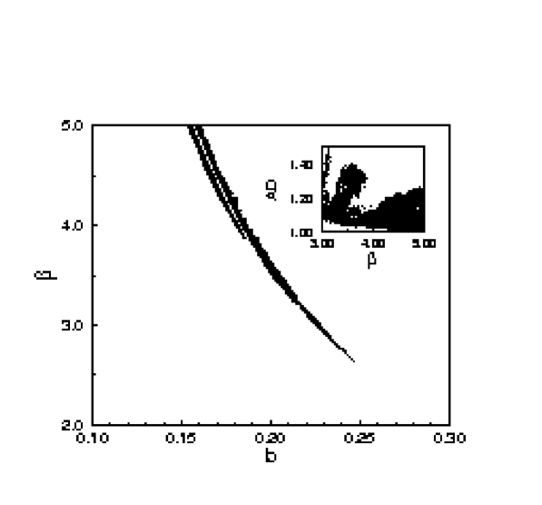
FIG. 1.: Analysis of a region in parameter space for hyperbolic-tangent transfer function and $N=2$. Points that lead to chaotic trajectories are marked. The remaining space in this region leads to stable attractors. The center of the circle at $(4.24,0.178)$ represents the chaotic point discussed in [10] . Insert: the attractor dimension (AD) of the chaotic points shown in this region. For each value of the parameter $\beta$, the AD of all the chaotic points along the $b$ axis are drawn.

FIG. 2.: A region in parameter space for hyperbolic-tangent transfer function and $N=3$. Points that lead to chaotic trajectories are marked. The remaining space in this region leads to stable attractors. Insert: A continuation of the main figure for smaller values of $b$ in a $\log$-$\log$ plot.

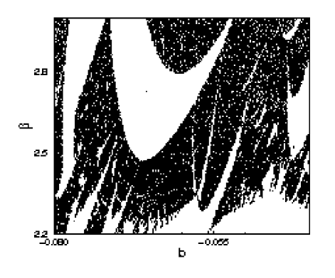
FIG. 3.: Example of a region in parameter space for hyperbolic-tangent transfer function and $N=9$ where points that lead to chaotic trajectories are marked. The remaining space in this region leads to stable attractors.

FIG. 4.: A sequence of period doubling bifurcations for a network with a $\sin$ transfer function and $N=3$. The weights consist of a single Fourier component without phase and bias. The vertical axis, denoted by ‘amp’, is the actual amplitude value of the cycle in phase space. Insert: a blowup of the pointed region.

FIG. 5.: The difference $\Delta_{n}$ (Eq. (9)) for three cases. The lines are exponential fit of the data. The solid line represents the fit for $N=3$ with a slope of $4.69\pm 0.05$. The dashed line represents $N=4$ with a slope of $4.66\pm 0.02$ and the dotted line represents $N=4$ with an arbitrary weights with a slope of $4.65\pm 0.02$ .

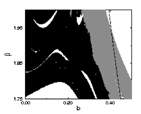
FIG. 6.: Analysis of a region in parameter space for a network with a $\sin$ transfer function and $N=2$ where points that lead to chaotic trajectories are marked. The dark(gray) colors correspond to areas with one(two) positive exponent. The remaining space in this region leads to stable attractors. The bold dashed line is the spine locus of the f.p. defined by Eq. (14), $n=0$.

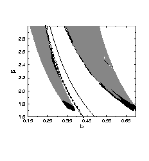
FIG. 7.: Analysis of a region in parameter space around the main spine loci for a $\sin$ transfer function and $N=2$. The initial condition in phase space is fixed to $S_{i}=1$. The dark(gray) color corresponds to areas with one(two) positive exponents. The remaining space in this region leads to stable attractors. The solid line is the spine locus of the f.p. defined by Eq. (14), and the solid line with circles is the calculated spine locus of the 2-cycle attractor defined by Eq. (15).

FIG. 8.: The attractor dimension (AD) as a function of the gain for a $\sin$ transfer function where $N=17$, $b=0$ and $\phi=0$. The solid curve is the AD and the dashed line below represents the number of positive exponents.

REFERENCES

- [1] E. Eisenstein, I. Kanter, D.A. Kessler and W. Kinzel, Phys. Rev. Lett. 74, 6 (1995).
- [2] I. Kanter, D.A. Kessler, A. Priel and E. Eisenstein, Phys. Rev. Lett. 75, 2614 (1995).
- [3] A. Priel, I. Kanter and D.A. Kessler, J. Phys. A 31, 1189 (1998).
- [4] A. Priel, I. Kanter and D.A. Kessler, in Advances in Neural Information Processing Systems, Vol. 10, edited by M.I. Jordan et. al. (Cambridge, MA: MIT Press, 1998), p. 315.
- [5] M. Schroder and W. Kinzel, J. Phys. A 31, 2967 (1998).
- [6] L. Ein-Dor and I. Kanter, Phys. Rev. E 57, 6564 (1998).
- [7] B. Soumitro, J.A. Yorke and C. Grebogi, Phys. Rev. Lett. 80, 3049 (1998).
- [8] J. Hertz, A. Krogh and R.G. Palmer, Introduction to the theory of neural computation (Addison-Wesley, Redwood City, CA, 1991).
- [9] E. Barreto, B.R. Hunt, C. Grebogi and J.A. Yorke, Phys. Rev. lett. 78, 4561 (1997).
- [10] C.S.O. Yokoi, M.J. Oliviera and S.R. Salinas, Phys. Rev. Lett. 54, 163 (1985).
- [11] An Ising system on a Cayley tree with infinite coordination limit and competing interactions between first (FM) and second (AFM) neighbors along an axial direction, is represented by a second order recursion relation for the magnetization per spin as Eq. (8).
- [12] J.G. Moreira and S.R. Salinas, J. Phys. A 20, 1621 (1987).
- [13] A. Priel (unpublished)
- [14] M.J. Feigenbaum, J. Stat. Phys. 19, 25 (1978).
- [15] P. Grassberger and I. Procaccia, Physica D 9, 189 (1983).
- [16] R. Dogaru R, A.T. Murgan, S. Ortmann and M. Glesner M, in Proceedings of the 1996 International Conference on Neural Networks, Washington, (IEEE, New-York, 1996).
- [17] J.L. Kaplan and J.A. Yorke, Comm. Math. Phys. 67, 93 (1979).
- [18] A. Wolf, J.B. Swift, H.L. Swinney and J.A. Vastano J A, Physica D 16, 285 (1985).