Low temperature behavior of the thermopower
in disordered systems near the Anderson transition
C. Villagonzalo and R. A. Römer
Institut für Physik, Technische Universität, D-09107 Chemnitz, Germany
Received 6 October 1998, revised 14 October 1998, accepted 15 October 1998 by U. Eckern
Abstract. We investigate the behavior of the thermoelectric power $S$ in disordered systems close to the Anderson-type metal-insulator transition (MIT) at low temperatures. In the literature, we find contradictory results for $S$. It is either argued to diverge or to remain a constant as the MIT is approached. To resolve this dilemma, we calculate the number density of electrons at the MIT in disordered systems using an averaged density of states obtained by diagonalizing the three-dimensional Anderson model of localization. From the number density we obtain the temperature dependence of the chemical potential necessary to solve for $S$. Without any additional approximation, we use the Chester-Thellung-Kubo-Greenwood formulation and numerically obtain the behavior of $S$ at low $T$ as the Anderson transition is approached from the metallic side. We show that indeed $S$ does not diverge.
Keywords: Thermoelectric power; Localization; Metal-insulator transition

1 Introduction

In this paper, we study the low temperature behavior of the thermoelectric power $S$ in disordered systems near the Anderson-type metal-insulator transition (MIT). In the framework of linear response theory, $S$, commonly abbreviated as the thermopower, is the coefficient that relates the temperature gradient in an open circuit with the induced electric field. In the metallic regime, the Sommerfeld theory states that $S$ is directly proportional to the negative temperature $-T$ [2]. But at a disordered-induced MIT, such as the Anderson transition in three dimensions (3D) [3], it is still not a settled issue how $S$ behaves at low $T$. Theoretical studies have either claimed that it diverges [4], or that it remains a constant [5] as the MIT is approached from the metallic side at low $T$. Moreover, comparing the results of the latter theory with that of experiments conducted on doped semiconductors [6] and on amorphous alloys [7] shows that measurements of $S$ are two orders of magnitude higher than those predicted in theory. Thus, it is of great interest to investigate the behavior of $S$ at low $T$ near the Anderson-type MIT. Here, for simplicity, we consider only the diffusion part of $S$, that is, we consider only the electronic contribution and neglect any possible electron-phonon interactions. In addition to $S$, we shall also compute thermal transport properties such as the thermal conductivity $K$ and the Lorenz number $L_{0}$.

2 Theoretical background

The derivation of the thermopower is based on the kinetic coefficients of the Chester-Thellung-Kubo-Greenwood formulation of linear response [8],

$$L_{ij}=(-1)^{i+j}\int_{-\infty}^{\infty}A(E)[E-\mu(T)]^{i+j-2}\left(-\frac{\partial f(E,\mu,T)}{\partial E}\right)dE\;\;\;\;\;\;\;i,j=1,2$$ (1)

where $E$ is the energy, $A(E)$ contains all the system-dependent features, $\mu(T)$ is the chemical potential, $f(E,\mu,T)=1/[1+\exp([E-\mu(T)]/k_{B}T)]$ is the Fermi function, and $k_{B}$ is the Boltzmann constant. These coefficients relate the electric field $\varepsilon$, concentration gradient $\nabla\mu$ and temperature gradient $\nabla{T}$ to the expectation values of the induced electric $\langle{\bf j}_{1}\rangle$ and heat $\langle{\bf j}_{2}\rangle$ current densities

$$\langle{\bf j}_{i}\rangle=|e|^{-i}\left[-L_{i1}({\bf\nabla}\mu-|e|\varepsilon)-L_{i2}T^{-1}{\bf\nabla}T\right]\;.$$ (2)

where $e$ is the electron charge. Measured under the assumption that there is no electric current and concentration gradient, the thermopower is thus given as

$$S=\frac{L_{12}}{|e|TL_{11}}\;.$$ (3)

The Anderson transition is then incorporated into the measurement of $S$ by setting the function $A(E)$ in the coefficient $L_{ij}$ as proportional to the critical behavior of the d.c. conductivity $\sigma$ at the MIT, that is,

$$A(E)=\left\{\begin{array}[]{cl}\alpha|E-E_{C}|^{\nu}&E\geq E_{C}\\ 0&E<E_{C}\end{array}\right.$$ (4)

where $\alpha$ is a constant, $\nu$ is the conductivity index and $E_{C}$ is the mobility edge. With this assignment the coefficient $L_{11}$ is simply $\sigma$. Furthermore, since $K$ is the coefficient that relates the temperature gradient to the induced heat current, it’s low temperature behavior at the MIT can be determined in a similar manner from $\langle{\bf j}_{2}\rangle$ with the assumption that there are no particle currents, and using the Anderson transition form of $A(E)$ as given above. Then the Lorenz number $L_{0}=(e/k_{B})^{2}\sigma/KT$ quickly follows. Thus, the low $T$ behavior of $S$, $K$ and $L_{0}$ at the Anderson transition follows easily after obtaining the kinetic coefficients, Eq. (1).

2.1 Divergent thermopower

A divergent $S$ at the Anderson transition $E=E_{C}$ is obtained if one uses the Sommerfeld expansion to get the low-$T$ leading contribution to $L_{ij}$ [4]. This method assumes that the chemical potential $\mu$ is equal to the Fermi energy $E_{F}$ even for finite $T$. However, $\mu=E_{F}$ only at $T=0$ [2]. A more serious approximation of the Sommerfeld expansion is the assumption that $A(E)$ is a smoothly varying function at $E=E_{C}$. This is not the case at the Anderson transition, as can be readily seen in Eq. (4).

2.2 Fixed-point thermopower

The approach proposed by Enderby and Barnes [5] evaluates the kinetic coefficients at $\mu=E_{C}$ for finite $T$, and afterwards the limit $T\rightarrow 0$ is taken. They find that the thermopower is a constant at the mobility edge for $T\rightarrow 0$, and is given by

$$S=-\frac{k_{B}}{|e|}\frac{(\nu+1)}{\nu}\frac{I_{\nu+1}}{I_{\nu}}$$ (5)

where $I_{1}=\ln 2$, $I_{\nu}=(1-2^{(1-\nu)})\Gamma(\nu)\zeta(\nu)$ for ${\mathrm{R}e}[\nu]>0,\;\nu\neq 1$, with $\Gamma(\nu)$ and $\zeta(\nu)$ the usual gamma and Riemman zeta functions. Hence, $S$ solely depends on $\nu$.

3 Calculation of the temperature dependent thermopower

One can determine the temperature dependence of the thermopower if one knows how $\mu$ varies with $T$. This information can be obtained from the number density $n$ of electrons at the MIT. In general, for any set of noninteracting electrons, the number density is defined as

$$n(\mu,T)=\int_{-\infty}^{\infty}dEg(E)f(E,\mu,T)\;,$$ (6)

where $g(E)$ is the density of energy levels per unit volume. Using the above equation, we numerically calculate $n$ using an averaged density of states $g(E)$ obtained by diagonalizing the Anderson model of localization. Earlier, we determined the averaged density of states for a 3D isotropic Anderson model with disorder $W=12$ [9]. Note that since our objective is to compare our theoretical results for $S$ with experimental measurements, such as those from amorphous alloys, the hopping parameter $t$ is of the order of 1 eV. Hence, we have expressed all energy units in terms of $t$ unless otherwise specified. We have selected the value of $W$ to be strong enough, such that we do not have singularities in the density of states. Yet, it should not be too strong, i.e. too close to the critical disorder. For this particular value of $W$, the value of $E_{C}$ is approximately $-7.5$, according to the mobility edge trajectory $E_{C}(W)$ calculated in Ref. [10]. The conductivity index $\nu$ is $\approx 1.3$, according to a current numerical estimate [11]. Then we integrate the density of states for $E\leq E_{F}$ to obtain the corresponding value of $n$ for a given value of $E_{F}$ at $T=0$. Keeping $n$ fixed at this value, we vary $T$ in Eq. (6) and numerically determine the variation of $\mu$. Using this information in Eq. (1), we solve for $L_{ij}$. It is then straightforward to determine $S$ for a particular value of $E_{C}$ from Eq. (3).

4 Results and discussion

In Fig. 1, the temperature dependendence of the chemical potential is shown together with the averaged density of states from which it was measured. Note that from this smooth density of states, we obtain a $T$ dependence of $\mu$ which barely changes when one selects $E_{F}$ in the metallic or the localized region. However, its slope changes much faster as compared to the chemical potential from a free electron gas as shown in Fig. 1. Note that this free electron result was also similarly obtained from the same expression for $n$ given in Eq. (6), but using the Sommerfeld expansion in order to obtain $\mu$.

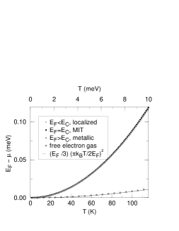
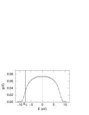
Fig. 1: Top: The low $T$ behavior of $\mu$. Near the MIT, $\mu(T)$ is similar in both the localized and the metallic regions. Bottom: The averaged density of states of a 3D isotropic Anderson model with $W=12$. For clarity only every 10th data point is marked by a symbol ($\circ$).

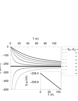
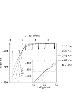
Fig. 2: Top: The low $T$ behavior of $S$. Note that $S$ does not diverge at the MIT as $T\rightarrow 0$. Bottom: Same data as in the top panel, plotted with respect to $\mu$ for different Fermi energies. The lines connect isotherms of $S$. As shown in the inset, $S$ is a fixed point at the MIT.

Next, Fig. 2 shows our thermopower measurements. The curves at the top of Fig. 2 clearly show the MIT, the dividing line between the metallic ($E_{F}>E_{C}$) and localized ($E_{F}<E_{C}$) regions. As $T\rightarrow 0$, $S$ gets more negative in the localized region, while $S\rightarrow 0$ in the metallic region. As we move further away from the MIT towards the metallic region at low $T$, $S$ behaves as expected from the Sommerfeld theory, that is, linearly proportional to $-T$. This indicate nonzero values of $\sigma(E_{F})$ confirming the metallic nature in this energy region. More importantly, we see that $S$ is a constant at the MIT, $E_{F}=E_{C}$. As $T\rightarrow 0$, it approaches the value -228.4 ${\mu}V/K$. This value agrees with the $T$-independent value for $\nu=1.3$ as predicted by Eq. (5). At the MIT, a negative $S$ value of the order of hundreds of ${\mu}V/K$ has never been experimentally observed to the best of our knowledge. To see the $T$-independence of $S$ at the MIT, we refer to the bottom of Fig. 2. Here we show the behavior of $S$ at different Fermi energies for different temperatures. It is clearly demonstrated in the inset that for different values of $T$, $S$ is a fixed point at the MIT ($\mu=E_{C}$) verifying what Enderby and Barnes had previously concluded [5].

Similarly, we have studied the other thermal transport properties $K$ and $\sigma$. Our preliminary investigation shows that $K\rightarrow 0$ as $T\rightarrow 0$ at any energy region. Furthermore, in the metallic phase, $L_{0}$ approaches the value $\pi^{2}/3$ which according to the law of Wiedemann and Franz is a universal value for all metals (see for example Refs. [2, 8]). At the MIT, however, $L_{0}$ has a value dependent only on the conductivity index $\nu$. Detailed results of these transport properties will be discussed elsewhere.

5 Conclusions

In this work we have studied the low temperature behavior of the thermoelectric power for the 3D isotropic Anderson model close to the MIT. We have numerically obtained the temperature dependence of the chemical potential necessary to solve for $S$ from the general expression of the number density for any set of noninteracting electrons. We have shown that $\mu(T)$ is very similar regardless which energy region close to the MIT one considers. Using this result and the Chester-Thellung-Kubo-Greenwood formulation, our calculations yield a sharp contrast of the $S$ behavior between metallic and localized regions clearly outlining the MIT. Finally, as the MIT is approached from the metallic side $S$ is a fixed point. As $T\rightarrow 0$ at the MIT, $S$ approaches the fixed-point value predicted by Enderby and Barnes which for $\nu=1.3$ is $S=-228.4\;{\mu}V/K$. Therefore, we have established that as the MIT is approached at low $T$ the thermopower does not diverge but remains a constant. Its fixed-point value depends only on the critical behavior of $\sigma$. How $S$ behaves for varying degrees of disorder is a subject of further investigation.

We thank T. Vojta for helpful discussions. We also gratefully acknowledge financial support by the DFG through Sonderforschungsbereich 393.

References

- [1]
- [2] N. W. Ashcroft, N. D. Mermin, Solid State Physics, Saunders College, New York, 1976
- [3] P. W. Anderson, Phys. Rev. 109 (1958) 1492
- [4] U. Sivan, Y. Imry, Phys. Rev. B 33 (1986) 551; C. Castellani, C. Di Castro, M. Grilli, G. Strinati, Phys. Rev. B 37 (1988) 6663
- [5] J. E. Enderby, A.C. Barnes, Phys. Rev. B 49 (1994) 5062
- [6] M. Lakner, H. v. Löhneysen, Phys. Rev. Letters 70 (1993) 3475
- [7] C. Lauinger, F. Baumann, J. Phys.: Condens. Matter 7 (1995) 1305
- [8] G. V. Chester, A. Thellung, Proc. Phys. Soc. 77 (1961) 1005; R. Kubo, J. Phys. Soc. Japan 12 (1957) 570; D. A. Greenwood, Proc. Phys. Soc. 71 (1958) 585
- [9] F. Milde, R. A. Römer, M. Schreiber, Phys. Rev. B 55 (1997) 9463
- [10] H. Grussbach, M. Schreiber, Phys. Rev. B 51 (1995) 663
- [11] B. Kramer, A. MacKinnon, Rep. Prog. Phys. 56 (1993) 1469