Scaling properties of discrete fractals

Abstract

An important problem in the analysis of experimental data showing fractal properties, is that such samples are composed by a set of points limited by an upper and a lower cut off. We study how finite size effect due to the discreteness of the sets may influence self similar properties even far from these cut-offs. Estimations of these effects are provided on the basis of the characteristics of the samples. In particular we present an estimate of the length scale above which information about average quantities is reliable, by explicitly computing discreteness effects in number counting . The results have particular importance in the statistical analysis of the distribution of galaxies.

The simplest way to characterise a fractal structure is to analyse the scaling behaviour on large sets of data, of convenient averaged quantities, such as the two point correlation function [1, 2]. Here, we introduce a more complete description of self similar structures by including the properties of the fluctuations of such quantities with respect to the average values. Previous approaches to this problem include the analysis of the void distribution [3, 4] and analysis of the tree points correlation function [5].

In order to introduce a theory of the fluctuations in fractal patterns, it is crucial to characterize the finite size effects [6]. Real data [7] are sets of a finite number of points where fluctuation analysis requires much larger samples than those needed to compute the averaged quantities. In particular in the field of large scale structure astrophysics, due to observational limitations, unaveraged quantities are widely used in the statistical analysis of galaxy correlations [1, 8, 9].

In this work we further develop fluctuation analysis and give quantitative criteria to define its statistical significance for a given data set. In order to proceed with this analysis we distinguish between finite size effects related to the shape of the data set boundaries and the finite size effects due to the discreteness of the sample. In order to avoid the former we carefully select the region for number counting. To approach the latter we compute the probability distribution of fluctuations in number counts on a discrete set of points.

The scaling quantity we will consider is the conditional average number mass $N(r)$ defined below. Given a set of $N_{tot}$ points, let $n_{i}(r)$ be the Conditional number Mass (CM) from the point $i$ defined as follows:

$$n_{i}(r)=\int_{S(r,i)}\sum_{j}\delta({\bf x-x}_{j})d^{d}{\bf x}\;,$$ (1)

where $j$ runs over all the points in the set and $S(r,i)$ is the $d$-dimensional hypersphere with radius $r$ centred at the point $i$. $N(r)$ at a given $r$ is defined as the average of the CM’s over all the points whose distance from the sample boundaries $\bar{r}_{i}$ is greater than $r$:

$$N(r)=\left<n_{i}(r)\right>_{\bar{r}_{i}>r}\;.$$ (2)

The supplementary condition is needed in order to avoid the finite size effects linked to the geometrical shape of the sample as pointed out in Ref.s [10, 9]. With this restriction we now can face the problem of the discreteness of the data set.

For a fractal set of dimension $D$, $N(r)$ takes the form [1]:

$$N(r)=Br^{D}\;,$$ (3)

where $B$ is a prefactor independent from $D$. In fig. 1, we compare the behaviour of a single CM to $N(r)$ for one of the fractal sets described below. The multiplicative character of fluctuations is reflected in their constant amplitude in the log-log plot. In order to compare fluctuations at different scales we introduce the normalized conditional number:

$$f_{i}(r)=\frac{n_{i}(r)}{N(r)}\;.$$ (4)

For $N(r)\gg 1$ it is possible to introduce a continuous representation for the variable $f$, whose associated probability distribution ${\cal P}(f)$ is independent from $r$ due to the self-similarity. On the other hand one expects the continuous limit does not to hold at a scale close to the lower cut-off. This is because in such a range the CM can take only a small set of discrete values corresponding to the presence of $0,1,2...$ points inside the $d$-dimensional hypersphere. For this reason, it is possible to observe fluctuations not scale invariant at small scales even if the averaged quantities show the correct scaling behaviour. The effect of the discreteness on fluctuations is particularly evident when fractal correlations are present at distances much smaller than the typical distance between neighbor points. Samples with this property are equivalent to sets of randomly picked points from much larger fractals.

Generally, the probability $\Pi(n,r)$ of find $n$ points inside a $d$-dimensional hypersphere of radius $r$ centered on a point of the set, is the convolution of the scale invariant distribution density ${\cal P}(f)$ with a Poisson distribution $P_{m}(n)$ with average $m=fN(r)=fBr^{D}$:

$$\Pi(n,r)=\int\limits_{0}^{\infty}df{\cal P}(f)P_{fN(r)}(n)=\left<P_{fN(r)}(n)\right>_{f}\;,$$ (5)

where the notation $\left<\phi(f)\right>_{f}\equiv\int\limits_{0}^{\infty}df{\cal P}(f)\phi(f)$ stands for the average with respect to the distribution function ${\cal P}(f)$. We define also $\left<\phi(n)\right>_{n}\equiv\sum_{n=0}^{\infty}P_{fN(r)}(n)\phi(n)$ for the average with respect to the Poisson distribution. The variance of the number of points $n$ is then:

$$\sigma^{2}(r)=\sum_{n=0}^{\infty}\Pi(n,r)n^{2}-N^{2}(r)=\left<\left<n^{2}\right>_{n}\right>_{f}-N^{2}(r)\;,$$ (6)

where in the last equality we exchanged the sum with the integral. Inserting eq. (5) in eq. (6), adding and subtracting the quantity $\left<\left(fN(r)\right)^{2}\right>_{f}$ we obtain:

$$\sigma^{2}(r)=\left<\left<n^{2}-f^{2}N^{2}(r)\right>_{n}\right>_{f}+\left<f^{2}N^{2}(r)-N^{2}(r)\right>_{f}\;.$$ (7)

This gives:

$$\sigma^{2}(r)=N(r)+N^{2}(r)\sigma^{2}_{si}\;,$$ (8)

where $\sigma^{2}_{si}$ is the variance of scale invariant distribution ${\cal P}(f)$. In the first term of eq. 7, the inner average is the variance of poisson distribution, i.e. $fN(r)$, and the outer average with respect $f$ will give $N(r)$.

This expression gives the relation between the variance of the number of points in a discrete fractal set with respect the intrinsic variance of the fractal probability distribution ${\cal P}(f)$. The variance of the fluctuations is then:

$$\sigma^{2}_{f}(r)\equiv\frac{\sigma^{2}(r)}{N^{2}(r)}=\sigma^{2}_{si}+\frac{1}{N(r)}\;,$$ (9)

where the effect of the random sampling is simply to add the Poisson contribution $1/N(r)$ to the scale invariant term $\sigma^{2}_{si}$. Through the expression in eq.(9) it is possible to evaluate $\sigma^{2}_{si}$ at any scale. Moreover we can estimate the scale beyond which the poisson fluctuations are negligibile with respect the intrinsic ones. In order to have the Poisson term i.e. $10$ times smaller than the intrinsic one, the CM should be fitted for $r$ larger than the minimal statistical length $\lambda$:

$$\lambda=\left(\frac{10}{B\sigma_{si}^{2}}\right)^{\frac{1}{D}}\;.$$ (10)

Eq. (10) with $\sigma_{si}^{2}=1$ has been derived in a phenomenological way in the context of large scale structure of the Universe [11, 9]. The quantity $\sigma^{2}_{f}(r)$ has been called lacunarity [2], and is usually referred to as one of the intrinsic characterisation of a fractal set. However the scale invariant value $\sigma_{si}^{2}$ appear only in the $r\gg\lambda$ region.

Having defined this quantity, it is possible to further characterise the fractal set. This is done by noticing that fluctuations show a characteristic “correlation length” on a $log-log$ scale. This corresponds to a correlation scale difference $\Delta S$ above which fluctuations are uncorrelated and can be used as an estimate of limiting “length” that has to be considered in order to deal with reliable data.

The correlation function between fluctuations at scales $r_{1}$ and $r_{2}$ is:

$$\tilde{S}(r_{2},r_{1})=\left<(f(r_{2})-1)(f(r_{1})-1)\right>\equiv\left<\delta f(r_{2})\delta f(r_{1})\right>\;.$$ (11)

In the self similar regime one expects $\tilde{S}$ to be a function of the ratio of the scales, i.e. $\tilde{S}(r_{2},r_{1})=S(\log_{10}(r_{2}/r_{1}))\equiv S(\Delta)$. An estimation for $S(\Delta)$ may be found in the following way: let $n_{i}(r_{1})$ the CM from the point $i$ up to a scale $r_{1}$, $n_{i}(r_{2})$ the CM up to a scale $r_{2}>r_{1}$ and $\tilde{n_{i}(r_{1},r_{2})}$ the number of points in the shell $r_{2}-r_{1}$. We can express $\delta f_{i}(r_{2})$ in the following way:

$$\delta f_{i}(r_{2}) = f_{i}(r_{2})-1=\frac{n_{i}(r_{2})}{N(r_{2})}-1=\frac{n_{i}(r_{1})+\tilde{n}(r_{1},r_{2})}{N(r_{1})}\cdot\frac{N(r_{1})}{N(r_{2})}-1=$$

$$= {f_{i}(r_{1})}\frac{r_{1}^{D}}{r_{2}^{D}}-1+\frac{\tilde{n}(r_{1},r_{2})}{N(r_{2})}=\delta f_{i}(r_{1})+\delta\tilde{f}(r_{1},r_{2})\;.$$

Assuming that the number of points in the $r_{2}>r_{1}$ shell, $\tilde{n}_{i}(r_{1},r_{2})$ is uncorrelated with $n_{i}(r_{1})$, we have that $\left<\delta f_{i}(r_{1})\delta\tilde{f}_{i}(r_{1},r_{2})\right>=0$. Therefore:

$$S\left(\Delta\right)\!=\!\left<\!\!\delta f(r_{1})\left(\delta f(r_{1})\frac{r_{1}^{D}}{r_{2}^{D}}\right)\!\!\right>=\sigma^{2}_{f}\left(\frac{r_{1}}{r_{2}}\right)^{D}\!\!=\sigma^{2}_{f}\cdot 10^{-\frac{\Delta}{\Delta_{c}}}\;,$$ (13)

where $\Delta_{c}=D^{-1}$. In the general case $\left<\delta f_{i}(r_{1})\delta\tilde{f_{i}}\right>>0$ and then eq. (13) is the lower limit.

To show the applicability of the formulae derived we will analyse selected fractal samples. Those fractal sets are obtained picking randomly points from larger samples generated by a random $\beta$ model (RBM) algorithm [12] in two dimensions. The original sets contain from $10^{9}$ to $10^{10}$ points, while the diluted samples contain around $10^{7}$ points, in a square domain of side 2.

Two characteristic lengths for the sets are respectively the minimal possible distance between points $\epsilon$ (which corresponds also to the minimal distance at which one observes fractal correlations), and the average distance to the nearest point $r_{0}$, which is related to the prefactor $B$ through $r_{0}^{D}\sim B^{-1}$. Whilst the two lengths may differ substantially for highly diluted samples, they are almost identical for the RBM without dilution.

In fig 1, we show $N(r)$ for a RBM fractal with $D=0.5$, $\epsilon\sim 10^{-15}$, $r_{0}\sim 10^{-14}$. The dotted line is the theoretical behaviour for $N(r)$ in this sample and the open circles are the values for the CM from a randomly chosen point.

In fig. 2 is reported the quantity $\sigma_{f}^{2}(r)$ for two sets of data: the fractal with $D=0.5$ and another one with $D=1.8$ ($\epsilon\sim 10^{-5}$ and $r_{0}\sim 10^{-4}$). In eq.(9) we take as independent variable the $N(r)$; in this way it is possible to fit the data to eq. (9) with a single parameter $\sigma^{2}_{si}$ (solid lines). The $N^{-1}(r)$ scaling is the Poissonian term and the plateau gives the intrinsic value $\sigma^{2}_{si}$. At large $N(r)$ deviations from the theoretical behaviour are observed. The reason for that may be understood through the following argument. All the points belonging to a cluster of size $r_{c}$ have correlated $n_{i}(r)$ for $r>r_{c}$. Sample independent behaviour of fluctuations is obtained for $r\sim r_{c}$ as long as a large number of independent clusters of size $r_{c}$ is contained in the sample volume. This condition is less and less fulfilled as $r$ increases. This gives rise to a strong reduction of $\sigma^{2}_{f}(r)$ whilst approaching the sample size. In the insert, we show the distributions of the fluctuations in the scale invariant regions, ${\cal P}(f)$, for the two samples.

In fig. 3 we show the probability distribution for the fluctuations $f$ at various $r$, for the $D=1.8$ fractal. Continuous lines refer to $r$ in the range $[10^{-3}$-$10^{-2}]$ where the good superposition of the different curves signals the scale invariance of the fluctuations. Outside from this region the measured distribution deviates from the intrinsic shape. The histogram of fig 3 is the probability distribution at smaller scales ($\sim 10^{-4}$), out from the scale invariant regime . The main features of it are the discreteness of the allowed value for $f$ and the larger variance due to the Poisson noise as explained before.

Fig 4 shows the measure of correlation between fluctuations $S(r_{1}/r_{2})$ at different scales. The points refer to three fractal sets with respectively fractal dimension $D=0.5,1,1.8$ and are the average of $S(r_{2}/r_{1})$ for all $r_{1}$ and $r_{2}$ inside the scale invariant range. While for small fractal dimension, $D=0.5$, the values estimated from eq. (13) are in rather good agreement with the data, the sets with $D$ closer to the dimension of the embedding space ($D=1.8$) show higher additional correlations between fluctuations at different scales. According to eq. (13) we may estimate the correlation scale difference to be $\Delta_{c}\sim D^{-1}$ for small fractal dimension. On the other hand for large dimensions, $\Delta_{c}$ appears not to decrease below $1$. An estimation for the correlation scale difference in the two dimensional RBM is:

$$\Delta_{c}=\mbox{Max}\left(1,\,\frac{1}{D}\right)\;.$$ (14)

Recovering the average behaviour of $N(r)$ from the measure of single $n_{i}(r)$ requires then a range of scale larger then $\Delta_{c}$.

The main result is that this analysis allows one to specify the value of $\Delta_{c}$. Thereby introduces a measure for a quantity which has been customary to define as “large enough” [7]. For instance, the fractal with dimension $D=0.5$ has $\Delta_{c}=2$ and in fig. 1 the corresponding CM shows typical length of fluctuations of $2-3$ orders of magnitude.

A direct application of such results is in the study of statistical properties of galaxy distribution. Here, a fundamental measure is the the counts of galaxies versus the distance from the Earth, or galaxy CM, $n_{E}(r)$. The interpretation of the behaviour of galaxy CM is crucial in the debate about the existence or not of the homogeneity scale of galaxy distribution in the Universe, which is one of the pillars of standard Big Bang theory. On the other side, the amount of available data are not so large, making important to check for finite size effects.

In conclusion, the intrinsic distribution of the fluctuations ${\cal P}(f)$ can be measured only for scales greater than the minimal statistical length, defined in eq. (10). On the other hand, the lacunarity of a discrete fractal may be evaluated, at all scales, as $\sigma_{f}^{2}(r)$. In those cases in which the CM has to be used in extracting fractal parameters from experiments, data for $r<\lambda$ have to be discarded and a range of scale larger than $\Delta_{c}$ is needed.

It is a great pleasure to acknowledge G.Caldarelli for critical reading of the manuscrpt and for many suggestions and discussions. We would also acknowledge A. Gabrielli, M.Joyce, M. Muñoz, L. Pietronero and F.Sylos Labini for valuable discussions and critical comments. This work has been partially supported by EEC TMR Network “Fractal Structure and self-organization” ERBFMRXCT980183.

fig1.ps

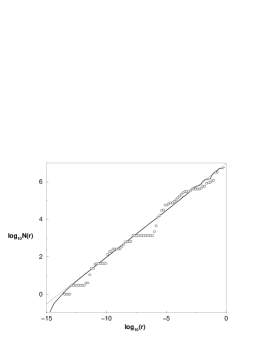
Fig. 1.–: The solid line is the logarithmic conditional average number of points as function of the logarithmic distance for a random $\beta$ model with dimension $D=2$ and $10^{7}$ points. Open circles are the counts from one point picked randomly. The dotted line is the theoretical power law expected. The small deviations from the power law at small and large scales are due to different kinds of finite size effects.

fig2.ps

Fig. 2.–: Reduced variance vs. the average number of points, logarithmic scale. Squares refer to a RBM with $D=1.8$ and circles to one with $D=0.5$. The solid and the dashed lines are fitted to eq. (9). In the inset are shown the numerical ${\cal P}(f)$ for the two sets above.

fig3.ps

Fig. 3.–: Solid lines refer to the numerical probability density of the fluctuation at several different scales within the range of self similarity ($D=1.8$). The histogram is the same quantity at smaller scales, in the regime where the discretization of $f$ and the Poisson noise are much more relevant.

fig4.ps

Fig. 4.–: Correlation between fluctuation versus the scale difference. Circles, squares and diamonds refer to fractals with $D=0.5,1,1.8$ respectively. Lines are fitted to eq. (13).

References

- [1] Mandelbrot B. B. , in The fractal Geometry of Nature , edited by Freeman, (San Francisco) 1982.
- [2] Falconer K.J., in Fractal Geometry: Mathematical Foundation and Application, edited by John Willey and sons, (New York) 1990.
- [3] Mandelbrot B.B., Progress in Probability, 37 (1995) 15.
- [4] Gefen Y. et al.: , Phys. Rev Lett., 45 (1980) 855; Y. Gefen , J. Phys. A, 17 (1984) 1277.
- [5] Blumenfeld R. and Ball R.C., Phys. Rev E, 47 (1993) 2298.
- [6] Grassberger P., Phys Lett. A, 128 (1988) 369.
- [7] Avnir D., Biham O.,Lidar D.A. and Malcai O., Science, 279 (1998) 39.
- [8] Peebles P.J.E., in Principles of Physical Cosmology, edited by Princeton University Press, (Princeton) 1993.
- [9] Sylos Labini F., Montuori M. and Pietronero L., Physics Reports, 293 (1998) 61 .
- [10] Coleman P.H.and Pietronero L., Physics Reports, 213 (1992) 311.
- [11] Montuori M.,Sylos-Labini F., Gabrielli A., Amici A. and Pietronero L., Europhys. Lett., 39 (1997) 103 .
- [12] Benzi R.,Paladin G.,Parisi G. and Vulpiani A. , J. Phys., A17 (1984) 3521.