Dynamics of spherical particles on a surface:
About collision induced sliding and other effects

Abstract

We present a model for the motion of hard spherical particles on a two dimensional surface. The model includes both the interaction between the particles via collisions, as well as the interaction of the particles with the substrate. We analyze in details the effects of sliding and rolling friction, that are usually overlooked. It is found that the properties of this particulate system are influenced significantly by the substrate-particle interactions. In particular, sliding of the particles relative to the substrate after a collision leads to considerable energy loss for common experimental conditions. The presented results provide a basis, that can be used to realistically model the dynamical properties of the system, and provide further insight into density fluctuations and related phenomena of clustering, structure formations, and inelastic collapse.

]

I Introduction

In this paper we address the problem of the motion of a set of hard spherical particles on an inclined, in general dynamic surface. While there have been substantial efforts to understand in more details the problem of the nature of interaction of a single particle with the substrate [2, 3, 4, 5, 6, 7, 8, 9, 10, 11], these efforts have not being extended to the multiparticle situation. On the other hand, there has been recently a lot of interest in one [12, 13, 14, 15, 16, 17] or two [18, 19, 20, 21, 22, 23, 24, 25] dimensional granular systems. These systems are of considerable importance, since they provide useful insight into more complicated systems arising in industrial applications, and also because of many fascinating effects that occur in simple experimental settings and theoretical models. Theoretical and computational efforts have lead to results including density fluctuations, clustering, and inelastic collapse [13, 14, 15, 17, 18, 19, 20, 21]. Further, a system of hard particles energized by either an oscillating side wall, or by oscillating surface itself, has been explored recently [15, 17, 21]. This system, due to its similarity to one or two dimensional gas, appears to be a good candidate for modeling using continuous hydrodynamic approach [15, 17, 21].

It is of great interest to connect theoretical and computational results with experimental ones. Very recently, it has been observed experimentally that many complex phenomena occur in the seemingly simple system of hard particles rolling and/or sliding on a substrate. In particular, clustering [22, 23], and friction-based segregation [23] have been observed. While some of the experimental results (e.g. clustering) could be related to the theoretical results [21], there are still considerable discrepancies. Theoretically, it has been found that the coefficient of restitution, measuring the elasticity of particle-particle collisions, is the important parameter of the problem, governing the dynamical properties of the system. While the coefficient of restitution is definitely an important quantity, a realistic description of an experimental system cannot be based just on this simple parameter. As pointed out in [22], the rotational motion of the particles and the interaction with the substrate introduce an additional set of parameters (e.g. the coefficients of rolling and sliding friction), that have not been included in the theoretical descriptions of the system.

Our goal is to bridge this gap between experiment and theory, and formulate a model that includes both particle-particle and particle-substrate interactions, allowing for a comparison between experimental and theoretical results. Specifically, we address the phenomena of rolling friction and sliding, that lead to the loss of mechanical energy and of linear and angular momentum of the particles. In order to provide a better understanding of the importance of various particle and substrate properties that define the system (e.g. rolling friction, sliding, the inertial properties of the particles), we concentrate part of the discussion on monodisperse, hard (steel), perfectly spherical solid particles, moving on a hard (aluminum, copper) substrate [22, 23, 24]. However, through most of the presentation, the discussion is kept as general as possible, and could be applied to many other physical systems. Specifically, the extension of the model to more complicated systems and geometries is of importance, since most of the granular experiments involve some kind of interaction of the particles with (static or dynamic) walls. In particular, the discussion presented here is relevant to wall shearing experiments, where particle-wall interactions are of major importance in determining the properties of the system (see [26] and the references therein).

In section II we explore all of the forces that act on the particle ensemble on a moving, inclined substrate. First we explore particle-particle interactions, and formulate a model incorporating the fact that the particles roll on a surface, and have their rotational degrees of freedom considerably modified, compared to “free” particles. Further, we include the interaction of the particles with the substrate, paying attention to the problem of rolling friction and sliding. The analysis is extended to the situation where the substrate itself is moving with the prescribed velocity and acceleration. Because of the complexity of the interactions that the particles experience, we first consider the problem of particles moving without sliding, and include the sliding at the end of the section. In section III, we give the equations of motion for a particle that experiences collisions with other particles, as well as interaction with the substrate. In Section IV we apply these equations of motion to the simple case of particles moving in one direction only. It is found that many interesting effects could be observed in this simple geometry. In particular, we explore the effect of sliding both during and after the collisions, and give estimates for the experimental conditions that lead to sliding. Finally, we give the results for the time the particles slide after a collision, as well as for the sliding distance, and for the loss of the translational kinetic energy and linear momentum of the particles.

II Forces on particles

Particles moving on an inclined hard surface experience three kind of forces:

• Body forces (gravity);

• Forces due to collisions with other particles and walls;

• Forces due to interaction with the substrate.

In what follows we analyze each of these forces, with emphasis on understanding the interaction between substrate and the particles. While the analysis is kept as general as possible, some approximations appropriate to the problem in question are utilized, in order to keep the discussion tractable. In particular, the coefficient of rolling friction is assumed much smaller then (static and kinematic) coefficients of sliding friction. Further, in this section the particles are confined to move on the substrate without jumping; the experimental conditions under which this extra degree of freedom is introduced are discussed in section IV. Throughout most of this section it is assumed that the particles are moving on the substrate without sliding; in section II C 3 we explain the conditions for sliding to occur.

In order to formulate a model that can be used for efficient molecular dynamics simulations, we choose rather simple models for the interactions between the particles and between the particles and the substrate. In modeling collisions between particles,, we neglect static friction, as it is often done [27, 28, 29, 30, 31, 32]. On the other hand, the static friction between the particles and the substrate is of major importance, since it leads to rolling particle motion; consequently, it is included in the model.

A Body forces

Here we consider only gravitational force that acts on the center of mass of the particles. It is assumed that there are no other (e.g. electrostatic) long range forces. In the coordinate frame that is used throughout (see Fig. 1), the acceleration of a particle due to gravity, $g$, is

$${\bf a}_{G}=-{\bf\hat{j}}\,g\sin(\theta)\ ,$$ (1)

where $\theta$ is the inclination angle.

FIG. 1.: The coordinate frame used in the paper.

B Collision forces

There are many approaches to modeling collision interactions between particles (see, e.g. [29, 33] and references therein). We note that rather complex models have been developed [34, 35, 36, 37, 38, 39, 40, 41, 42, 43], but choose to present a rather simple one, which, while necessary incomplete, still models realistically collision between particles moving with moderate speeds. In the context of the particles moving on a substrate, it is important to realize that, even though particles are confined to move on a 2D surface, the 3D nature of the particles is of importance. Even if one assumes that the particles roll on a substrate without sliding, only two components ($x$ and $y$) of their angular velocity, ${\bf\Omega}$, are determined by this constraint. The particles could still rotate with $\Omega^{z}$, which could be produced by collisions (hereafter we use ${\bf\Omega}$ to denote the components of angular velocity in $x-y$ plane only). We will see that rotations of the particles influence the nature of their interaction, as well as the interaction with the substrate.

Normal force. Using a simple harmonic spring model [29, 30, 33], the normal force on particle $i$, due to the collision with particle $j$, is given by

$${\bf F}_{N}^{c}=\left[k(d-r_{i,j})-\gamma_{N}\bar{m}({\bf v}_{i,j}\cdot{\bf\hat{n}})\right]{\bf\hat{n}}\ ,$$ (2)

where $k$ is a force constant, $r_{i,j}=|{\bf r}_{i,j}|$, ${\bf r}_{i,j}={\bf r}_{i}-{\bf r}_{j}$, ${\bf\hat{n}}={{\bf r}_{i,j}/r_{i,j}}$, ${\bf v}_{i,j}={\bf v}_{i}-{\bf v}_{j}$, $\bar{m}$ is the reduced mass, and $d=R_{i}+R_{j}$, where $R_{i}$ and $R_{j}$ are the radii of the particles $i$ and $j$, respectively. In this paper, we assume monodisperse particles, so that $d$ is equal to the diameter of a particle. The energy loss due to inelasticity of the collision is included by the damping constant, $\gamma_{N}$. The damping is assumed to be proportional to the relative velocity of the particles in the normal direction, ${\bf\hat{n}}$. While we use this simple linear model, the parameters $k$ and $\gamma_{N}$ are connected with material properties of the particles using nonlinear (Hertzian) model (see Appendix B). We note that $\gamma_{N}$ is connected with the coefficient of restitution, $e_{n}$, by $e_{n}=\exp({-\gamma_{n}t_{col}/2})$. Here $t_{col}$ is the collision time and is approximately given by $t_{col}\approx\pi\sqrt{m/(2k)}$ (see Appendix A). While more realistic nonlinear models lead to the velocity dependent coefficient of restitution [35, 42, 43], the linear model is satisfactory for our purposes, since we are interested in the collisions characterized by moderate impact velocities. In the case of particle-wall collisions, $d\rightarrow d/2$, ${\bar{m}}\rightarrow m$, and ${\bf r}_{i,j}\rightarrow{\bf r}_{wall}-{\bf r}_{i}$, where ${\bf r}_{wall}$ is the coordinate of the contact point at the wall.

Tangential force in $x-y$ plane. The motion of the particles in the tangential direction (perpendicular to the normal direction, in $x-y$ plane), leads to a tangential (shear) force. This force opposes the motion of the interacting particles in the tangential direction, so that it acts in the direction that is opposite to the relative tangential velocity, $v_{rel}^{t}$, of the point of contact of the particles. Both translational motion of the center of mass, and rotations of the particles with component of angular velocity in the ${\bf\hat{k}}$ direction contribute to $v_{rel}^{t}$, thus

$$v_{rel}^{t}={\bf v}_{i,j}\cdot{\bf\hat{s}}+{d\over 2}\;(\Omega_{i}^{z}+\Omega_{j}^{z})\ ,$$ (3)

where ${\bf\hat{s}}=({\bf\hat{n}}\cdot{\bf\hat{j}},-{\bf\hat{n}}\cdot{\bf\hat{i}})$. We model this force (on the particle $i$) by [29, 30]

$${\bf F}_{S}^{c}=sign(-v_{rel}^{t})min\left(\gamma_{S}\bar{m}|v_{rel}^{t}|,\nu_{k}|{\bf F}_{N}^{c}|\right){\bf\hat{s}}\ .$$ (4)

Here the Coulomb proportionality between normal and shear (tangential) stresses requires that the shear force, $|{\bf F}_{S}^{c}|$, is limited by the product of the coefficient of kinetic friction between the particles, $\nu_{k}$, and the normal force, $|{\bf F}_{N}^{c}|$. The damping coefficient in the tangential (shear) direction, $\gamma_{S}$, is usually chosen as $\gamma_{S}={\gamma_{N}/2}$, so that the coefficients of restitution in the normal and shear directions are identical [30]. An alternative method, where one models shear force by introducing a “spring” in the tangential direction, and calculates the force as being proportional to the extension of this spring, has been used as well (see, e.g. [33, 34]). We neglect static friction [27, 28, 29, 30, 31, 32, 42].

The torque on the particle $i$, due to the force ${\bf F}_{S}^{c}$, is ${\bf T}_{i}={\bf x}_{i}\times{\bf F}_{S}^{c}$, where ${\bf x}_{i}$ is the vector from the center of the particle $i$ to the point of contact, so ${\bf x}_{i}=-{d/2}\;{\bf\hat{n}}$. This torque produces the angular acceleration of the particle $i$ in the ${\bf\hat{k}}$ direction, $\dot{\Omega}_{i}^{z}={T_{i}^{z}/I}=-{d/(2I)}\,{\bf\hat{n}}\times{\bf F}_{S}^{c}$, where $I$ is the particles’ moment of inertia. Recalling that ${\bf F}_{S}^{c}$ is defined by Eq.(4), one obtains (we drop subscript $i$ hereafter, if there is no possibility for confusion)

$$\dot{\Omega}^{z}=-{d\over 2I}|{\bf F}_{S}^{c}|sign(v_{rel}^{t})\ .$$ (5)

By direct integration, this result yields $\Omega^{z}$. With this the relative velocity, $v_{rel}^{t}$ (Eq. (3)), is given, and hence we can calculate the tangential (shear) force, ${\bf F}_{S}^{c}$.

Tangential force in the ${\bf\hat{k}}$ direction. Since the particles are rolling, there is an additional force due to the relative motion of the particles at the point of contact in the perpendicular, ${\bf\hat{k}}$, direction. Figure 2 gives a simple example of the collision of two particles with translational velocities in the ${\bf\hat{i}}$ direction only. We model this force, ${\bf F}_{R}^{c}$, which is due to rotations of the particles with angular velocity, ${\bf\Omega}$, in the same manner as the shear force, ${\bf F}_{S}^{c}$. The force, ${\bf F}_{R}^{c}$, on the particle $i$ due to a collision with the particle $j$, acts in the direction opposite to the ${\bf\hat{k}}$ component of the relative velocity of the point of contact. Similarly to the “usual” shear force, we assume that the magnitude of ${\bf F}_{R}^{c}$ cannot be larger than the normal force times Coulomb coefficient; thus

$${\bf F}_{R}^{c}=sign(-v_{rel}^{z})min(\gamma_{s}{\bar{m}}|v_{rel}^{z}|,\nu_{k}|{\bf F}_{N}^{c}|){\bf\hat{k}}\ ,$$ (6)

and, for a general collision, $v_{rel}^{z}=R[({\bf\Omega}_{i}+{\bf\Omega}_{j})\times{\bf\hat{k}}]\cdot{\bf\hat{n}}$. In the case of a central collision as shown in Fig. 2, $v_{rel}^{z}$ simplifies to

$$v_{rel}^{z}=R({\bf\Omega}_{i}+{\bf\Omega}_{j})\cdot{\bf\hat{j}}\ .$$ (7)

FIG. 2.: The collision between two particles, with the linear velocities in the ${\bf\hat{i}}$ direction only. The direction of ${\bf F}_{R}^{c}$ follows from the assumption that $|{\bf v}_{j}|>|{\bf v}_{i}|$. The friction force ${\bf f}$ is explained in the following section. (The particles $i$ and $j$ are assumed to be in contact; for clarity reasons we show them separated).

The torque acting on the particle $i$ due to this force is ${\bf T}={\bf x}\times{\bf F}_{R}^{c}$. This torque produces an angular acceleration ${\bf\dot{\Omega}}={{\bf T}/I}$. Assuming that there is no sliding of the particles with respect to the substrate, we obtain the following result for the linear acceleration of the particle $i$

$${\bf a}_{R}^{c}=R{\bf\dot{\Omega}}\times{\bf\hat{k}}={R^{2}|F_{R}^{c}|\over I}\,sign(-v_{rel}^{z}){\bf\hat{n}}\ .$$ (8)

A 2D example given in Fig. 2 shows that ${\bf a}_{R}^{c}$ of both particles, $i$ and $j$, is in the direction of ${\bf\hat{n}}$, or $-{\bf\hat{i}}$ direction.

Let us also note that the force ${\bf F}_{R}^{c}$ modifies the normal force, ${\bf F}_{N}$, with which the substrate acts on the particle. From the balance of forces in the ${\bf\hat{k}}$ direction, it follows that the normal force is given by

$${\bf F}_{N}=mg{\bf\hat{k}}\cos(\theta)-{\bf F}_{R}^{c}\ .$$ (9)

The “jump” condition, $mg{\bf\hat{k}}\cos(\theta)={\bf F}_{R}^{c}$ is discussed in more details in section IV. Here we assume nonzero ${\bf F}_{N}$, and consider only the motion in $x-y$ plane.

To summarize, the collision interactions of the particle $i$ with the particle $j$ lead to the following expression for the total acceleration of particle $i$ (in $x-y$ plane)

$${\bf a}^{c}={\bf a}_{N}^{c}+{\bf a}_{S}^{c}+{\bf a}_{R}^{c}\ ,$$ (10)

where

$${\bf a}_{N}^{c}= {1\over m}\left[k(d-r_{i,j})-\gamma_{N}\bar{m}({\bf v}_{i,j}\cdot{\bf\hat{n}})\right]{\bf\hat{n}}\ ,$$ (11)

$${\bf a}_{S}^{c}= {1\over m}\,min\left(\gamma_{S}\bar{m}|v_{rel}^{t}|,\nu_{k}|{\bf F}_{N}^{c}|\right)\,sign(-v_{rel}^{t}){\bf\hat{s}}\ ,$$ (12)

$${\bf a}_{R}^{c}= {R^{2}\over I}\,min(\gamma_{s}{\bar{m}}|v_{rel}^{z}|,\nu_{k}|{\bf F}_{N}^{c}|)\,sign(-v_{rel}^{z}){\bf\hat{n}}\ .$$ (13)

Here ${\bf a}_{N}^{c}$ is the acceleration due to the normal force given by Eq. (2), ${\bf a}_{S}^{c}$ is the tangential acceleration due to the shear force, given by Eq. (4), and ${\bf a}_{R}^{c}$ is the rotational acceleration due to the tangential force in the ${\bf\hat{k}}$ direction, given by Eq. (6).

C Interaction with the substrate

The theory of rolling and sliding motion of a rigid body, even on a simple horizontal 2D substrate is complicated. For example, even though the question of rolling friction was addressed long ago [4], more recent works [5, 6, 7, 8, 9, 10, 11] show that there are still many open questions about the origins of rolling friction; similar observation applies to sliding friction. In order to avoid confusion, we use term “friction” to refer to either static or kinematic (sliding) friction; rolling friction is considered separately.

We approach this problem in several steps. After the introduction of the problem, we first consider a particle rolling without sliding, with vanishing coefficient of rolling friction, $\mu_{r}$. Next we present the generalization, that allows for nonzero $\mu_{r}$, as well as for the possibility of sliding. The substrate is assumed to move with its own prescribed velocity, ${\bf v}_{S}$, and acceleration, ${\bf a}_{S}$, which could be time dependent. The generalization to space dependent ${\bf v}_{S}$ and ${\bf a}_{S}$ is straightforward, but it is not introduced for simplicity. Similarly, we assume that the substrate is horizontal; the generalization to an inclined substrate is obvious.

Figure 3 shows the direction of the forces acting on a rolling particle. The friction force ${\bf f}$, that causes the particle to roll, acts in such a direction to produce the torque, ${\bf T}$, in the direction of the angular acceleration of the particle. Assuming that this friction force is applied to the instantaneous rotation axis, it does not lead to a loss of mechanical energy, as pointed out in [9]. If $\mu_{r}$ is zero, the particle will roll forever on a horizontal surface.

On the other hand, the rolling friction force, ${\bf f}_{r}$, acts in such a way to oppose the rotations. Thus it produces the torque, ${\bf T}_{r}$, in the direction opposite to the angular velocity of the particle. This torque could be understood if one assumes a small deformation of the substrate and/or particle, that modifies the direction of the rolling friction (reaction) force, ${\bf f}_{r}$, applied to the particle at a point slightly in front of the normal to the surface from the particle’s center [8, 9, 10, 44]. We note that this reaction force is actually our usual normal force, ${\bf F}_{N}$. While we include the rolling friction in the discussion, we neglect the small modification of the normal force due to the effect of rolling friction.

1 Rolling without sliding and without rolling friction

In this work, we ignore the complex nature (see e.g. [2, 3]) of the friction force, and assume that there is a single contact point between a particle and the substrate, with the friction force, ${\bf f}$, acting on the particle in the plane of the substrate, in the direction given by Newton’s law. In order to calculate the acceleration of the particle, we use the simple method given in [11]. The approach is outlined here, since in the later sections we will use the same idea in the more complicated settings.

If the substrate itself is moving, the friction force

$${\bf f}=m{\bf a}$$ (14)

is responsible for the momentum transfer from the substrate to the particle, where ${\bf a}$ is the particle acceleration. This force produces a torque (see Fig. 3)

$${\bf T}=-R\,{\bf\hat{k}}\times{\bf f}=I{\bf\dot{\Omega}}\ ,$$ (15)

where ${\bf\dot{\Omega}}$ is the angular acceleration of the particle. Assuming that there is no sliding, the velocity of the contact point is equal to the velocity of the substrate, ${\bf v}_{S}$ (this constraint will be relaxed in section II C 3, in order to model the more general case of rolling and/or sliding)

$${\bf v}_{S}={\bf v}+R\,{\bf\hat{k}}\times{\bf\Omega}\ .$$ (16)

Multiplying Eq. (15) by ${\bf\hat{k}}\times$ and using Newton law, we obtain

$${\bf a}={I\over mR}\,{\bf\hat{k}}\times{\bf\dot{\Omega}}\ .$$ (17)

Taking a time derivative of Eq. (16), and combining with Eq. (17), one obtains the following result for the acceleration of the center of the mass of the particle

$${\bf a}={1\over 1+{mR^{2}\over I}}{\bf a}_{S}\ .$$ (18)

Since, for a solid spherical particle, $I={2/5}\,mR^{2}$, we obtain ${\bf a}={2/7}\,{\bf a}_{S}$. So, the acceleration of a solid particle moving without rolling friction, or sliding, on a horizontal surface, is $2/7$ of the acceleration of the surface, ${\bf a}_{S}$ [11].

FIG. 3.: The forces and torques resulting from particle-substrate interaction. The friction force, ${\bf f}$, produces the torque, ${\bf T}$, in the direction of the angular acceleration of the particle; the rolling friction force, ${\bf f}_{r}$, produces the torque, ${\bf T}_{r}$, in the opposite direction, so that it leads to the decrease of the particle angular velocity, ${\bf\Omega}$. The deviation of ${\bf f}_{r}$ from the ${\bf\hat{k}}$ direction has been greatly exaggerated for the case of hard (e.g. metal) spherical particles.

2 Rolling without sliding with rolling friction

The rolling friction leads to the additional force, responsible for slowing down a particle on a surface. As already pointed out, this force produces the torque, ${\bf T}_{r}$, (see Fig. 3), in the direction opposite to the angular velocity of the particle, ${\bf\Omega}$. The origins of this force are still being discussed. The effects such as surface defects, adhesion, electrostatic interaction, etc., that occur at the finite contact area between the particle and the substrate [7], as well as viscous dissipation in the bulk of material [5, 6, 8] have been shown to play a role. Fortunately, for our purposes, we do not have to understand the details of this force, except that it decreases the relative velocity ${\bf{\bar{v}}}={\bf v}-{\bf v}_{S}$ of the particle with respect to the substrate. The acceleration of the particle due to this force, ${\bf a}_{R}$, is given by

$${\bf a}_{R}=-{\mu_{r}(|{\bf\bar{v}}|)|{\bf F}_{N}|\over m}{\bf{\hat{\bar{v}}}}\ ,$$ (19)

where the coefficient of rolling friction, $\mu_{r}(|{\bf\bar{v}}|)$, is defined by this equation, ${\bf{\hat{\bar{v}}}}={{\bf{\bar{v}}}/|{\bf{\bar{v}}}|}$, and ${\bf F}_{N}$ is the normal force. Alternatively, one could define the coefficient of rolling friction as the lever hand of the reaction force ${\bf f}_{r}$ shown in Fig. 3 [9]; for our purposes, the straightforward definition, Eq. (19), is more appropriate. For the case of steel spherical particles rolling on a copper substrate, the typical values of $\mu_{r}$ are of the order of $10^{-3}$ [22, 23]. Realistic modeling of the experiments where rolling friction properties are of major importance (such as recent experiment [23], which explores a system consisting of two kind of particles, distinguished by their rolling friction) requires accounting for velocity dependence of $\mu_{r}=\mu_{r}(|{\bf\bar{v}}|)$.

We note that there is an additional frictional force, which slows down the rotations of the particles around their vertical axes. While this additional force is to be included in general, we choose to neglect it here, since for the experimental situation in which we are interested [22, 23], the collisions between particles occur on a time scale that is much shorter than the time scale on which this rotational motion is considerably slowed down by the action of this frictional force (for other experimental systems, e.g. rubber spheres, this approximation would be unrealistic).

To summarize, a particle rolling without sliding on a horizontal surface experiences two kind of forces: first, the surface transfers momentum to the particle, “pulling” it in the direction of its own motion and leading to the acceleration, ${\bf a}$, given by Eq. (18). Second, due to the rolling friction, the particle is being slowed down, i.e. it is being accelerated with the acceleration, ${\bf a}_{R}$, in the direction opposite to the relative velocity of the particle and the substrate.

3 Rolling with sliding

Finally we are ready to address the problem of sliding. Sliding of a particle that is rolling on a substrate occurs when the magnitude of the friction force, resulting from Eq. (14), reaches its maximum allowed value $|{\bf f}_{max}|$, where

$$|{\bf f}_{max}|=\mu_{s}|{\bf F}_{N}|\ .$$ (20)

Here ${\bf F}_{N}$ is the normal force with which the substrate acts on a particle in the perpendicular, ${\bf\hat{k}}$, direction, and $\mu_{s}$ is the coefficient of static friction between a particle and the substrate. Once the condition (20) is satisfied, the friction force has to be modified, since now this force arises not from the static friction, but from the kinematic one. The direction of ${\bf f}$ is opposite to the relative (slip) velocity of the contact point of a particle and the substrate, ${\bf{\bar{u}}}$. Here ${\bf{\bar{u}}}={\bf u}-{\bf v}_{S}$, where ${\bf u}$ is the velocity of the contact point. The magnitude of ${\bf f}$ is equal to the product of the normal force and the coefficient of kinematic (sliding) friction, $\mu_{k}$

$${\bf f}=-\mu_{k}|{\bf F}_{N}|{\bf{\hat{\bar{u}}}}\ .$$ (21)

The typical range of values of $\mu_{s}$ and $\mu_{k}$ are $0.5-0.7$ and $0.1-0.2$, respectively. In the subsequent analysis we neglect rolling friction, since the rolling friction coefficient, $\mu_{r}$, is two orders of magnitude smaller than both $\mu_{s}$ and $\mu_{k}$.

The condition for sliding if there are no collisions. In this simple case, the friction force is given by Eqs. (14, 18). From the the condition for sliding, $|{\bf f}|=|{\bf f}_{max}|$, where $|{\bf f}_{max}|$ is given by Eq. (20), we obtain that the sliding occurs if

$$|{\bf a}_{S}|\geq\left(1+{mR^{2}\over I}\right){\mu_{s}\over m}|{\bf F}_{N}|\ .$$ (22)

As expected, if the substrate is accelerated with large acceleration, a particle slides. On a horizontal surface, the condition for sliding is $|{\bf a}_{S}|>|({\bf a}_{S})_{min}|$, where $|({\bf a}_{S})_{min}|=(1+{mR^{2}/I})\,\mu_{s}g$. For a solid steel sphere, $\mu_{s}\approx 0.5$, so $|({\bf a}_{S})_{min}|\approx 1.75\,g$. We note that this result does not depend on the diameter of a particle.

III Motion of the particles

The preceding section gives the results for the forces that the particles experience, because of their collisions, as well as because of their interaction with the substrate. Now we consider the mutual interaction of these effects and give expressions that govern the motion of the particles.

Similarly to before, we consider first the case where the particles roll without sliding. Sliding is included in the second part of the section.

A Motion without sliding

In this section, we do not include rolling friction, since its effect is rather weak compared to the effects due to the collisions and the substrate motion. It is important to note that this approximation is valid only during the collisions; in between of the collisions, the rolling friction force has to be included, since it is the only active force other than gravity.

The linear acceleration of a particle (in $x-y$ plane) is given by

$$m{\bf a}={\bf F}_{N}^{c}+{\bf F}_{S}^{c}+{\bf f}+m{\bf a}_{G}\ ,$$ (23)

where ${\bf F}_{N}^{c}$ and ${\bf F}_{S}^{c}$ are the forces on a particle due to the collision, in the normal and tangential directions, respectively; ${\bf f}$ is the friction force, and ${\bf a}_{G}$ is the acceleration due to gravity. Figure 2 shows a simple 2D example, where, for clarity, ${\bf F}_{S}^{c}$, the rolling friction force, and the rotations, characterized by $\Omega^{z}$, are not shown. The torque balance (generalization of Eq. (15)) implies that the angular acceleration of a particle is given by

$${\bf\dot{\Omega}}=-{R\over I}({\bf\hat{k}}\times{\bf f}+{\bf\hat{n}}\times{\bf F}_{R}^{c})\ ,$$ (24)

where we concentrate only on the rotations in the $x-y$ plane (the rotations characterized by $\Omega^{z}$ enter into the definition of ${\bf F}_{R}^{c}$ only). Following the same approach that led to Eq. (18), one obtains the result for the linear acceleration

$$m{\bf a}={{mR^{2}\over I}[{\bf F}_{N}^{c}+{\bf F}_{S}^{c}+({\bf\hat{k}}\cdot{\bf F}_{R}^{c}){\bf\hat{n}}]+m({\bf a}_{S}+{\bf a}_{G})\over 1+{mR^{2}\over I}}\ .$$ (25)

Similarly, one can solve for the friction force, ${\bf f}$, that the substrate exerts on a particle

$${\bf f}=-{{\bf F}_{N}^{c}+{\bf F}_{S}^{c}+m({\bf a}_{G}-{\bf a}_{S})-{mR^{2}\over I}({\bf\hat{k}}\cdot{\bf F}_{R}^{c}){\bf\hat{n}}\over 1+{mR^{2}\over I}}\ .$$ (26)

For a solid particle, one obtains

$$m{\bf a}={5\over 7}[{\bf F}_{N}^{c}+{\bf F}_{S}^{c}+({\bf\hat{k}}\cdot{\bf F}_{R}^{c}){\bf\hat{n}}]+{2\over 7}\,m({\bf a}_{S}+{\bf a}_{G})\ .$$ (27)

Eqs. (25, 27) effectively combine the acceleration due to the substrate motion, Eq. (18), and the acceleration due to the collisions, Eq. (10). We note that, due to the interplay between angular and linear motion of the particles, the total acceleration, given by Eq. (25), is not simply the sum of the accelerations due to the collisions, gravity, and the frictional interaction with the substrate. These interactions are effectively coupled, and one should not consider them separately.

B Motion with sliding

The condition for sliding follows immediately from Eq. (26), and from the sliding condition, $|{\bf f}|=|{\bf f}_{max}|$, yielding

$${\left|{\bf F}_{N}^{c}+{\bf F}_{S}^{c}-{mR^{2}\over I}({\bf\hat{k}}\cdot{\bf F}_{R}^{c}){\bf\hat{n}}+m({\bf a}_{G}-{\bf a}_{S})\right|\over 1+{mR^{2}\over I}}=\mu_{s}|{\bf F}_{N}|\ .$$ (28)

If this condition is satisfied, then ${\bf f}$ is given by Eq. (21).

Let us concentrate for a moment on the condition for sliding of a solid particle, on a horizontal static substrate, and neglect ${\bf F}_{R}^{c}$ and ${\bf F}_{S}^{c}$. The sliding condition is now given by $|{\bf F}_{N}^{c}|=(1+{mR^{2}/I})\,\mu_{s}|{\bf F}_{N}|$. As one would expect, this result resembles the condition for sliding due to the motion of the substrate, Eq. (22), since the two considered situations are analogous (the acceleration of the surface ${\bf a}_{S}$, plays the same role as the collision force, ${\bf F}_{N}^{c}$, scaled with the mass of a particle). Consequently, if the substrate is being accelerated in the direction of ${\bf F}_{N}^{c}$, a larger ${\bf F}_{N}^{c}$ is required to produce sliding. So, it is actually the relative acceleration of a particle with respect to the substrate motion which is relevant in determining the condition for sliding.

The effect of ${\bf F}_{R}^{c}$ on the sliding condition is more involved. Since ${\bf F}_{N}$ is connected with ${\bf F}_{R}^{c}$ via Eq. (9), ${\bf F}_{R}^{c}$ modifies both sides of Eq. (28). The net effect of ${\bf F}_{R}^{c}$ is discussed in some details in section IV.

If the sliding condition, Eq. (28), is satisfied, one has to relax the no-slip condition, Eq. (16). Instead of no-slip condition, we have

$${\bf u}={\bf v}+R\,{\bf\hat{k}}\times{\bf\Omega}\ .$$ (29)

If ${\bf u}={\bf v}_{S}$, the sliding velocity, ${\bf{\bar{u}}}={\bf u}-{\bf v}_{s}$, vanishes. The equation for the “sliding acceleration”, ${\bf\dot{\bar{u}}}$ (relative to the acceleration of the substrate, ${\bf a}_{S}$), follows similarly to Eq. (25),

$$m{\bf\dot{\bar{u}}}= \left(1+{mR^{2}\over I}\right){\bf f}+{\bf F}_{N}^{c}+{\bf F}_{S}^{c}-{mR^{2}\over I}({\bf\hat{k}}\cdot{\bf F}_{R}^{c}){\bf\hat{n}}$$ (31)

$$+m({\bf a}_{G}-{\bf a}_{S})\ .$$

To summarize, the linear acceleration of a particle is given by Eq. (23), where the normal force, ${\bf F}_{N}^{c}$, is given by Eq. (2) and the tangential force, ${\bf F}_{S}^{c}$, by Eq. (4). If there is no sliding, then the friction force, ${\bf f}$, is given by Eq. (26); on the other hand, if the sliding condition, Eq. (28), is satisfied, ${\bf f}$ is given by Eq. (21). Further, ${\bf a}_{S}$ is the acceleration of the substrate, and ${\bf a}_{G}$, the acceleration due to gravity, is given by Eq. (1). The angular acceleration of a particle, ${\bf\dot{\Omega}}$, is given by Eq. (24), where the rotational force due to the collision, ${\bf F}_{R}^{c}$, is given by Eq. (6). Finally, the sliding acceleration, ${\bf\dot{\bar{u}}}$, follows from Eq. (31). As mentioned earlier, the acceleration due to rolling friction, ${\bf a}_{R}$, is not important as long as much stronger collision, or friction forces, are present; it has to be added to the linear acceleration, ${\bf a}$, for realistic modeling of the motion of the particles between the collisions. The rotational motion of the particles, characterized by $\Omega^{z}$, enters into the model only by modifying the collision force between the particles in the tangential direction, ${\bf F}_{S}^{c}$.

The general expressions given in this section are used in the MD type simulations [25], in order to simulate the motion of a set of particles on an inclined plane. In this paper, we apply the results to a simple setting, and obtain the analytic results which provide better insight into the relative importance of various interactions. This is the subject of the next section.

IV Discussion

The analysis of the preceding section gives rather general results, that provide all the information needed for modeling of the particles’ motion. On the other hand, the complexity of the final results obscures simple physical understanding. In this section, we concentrate on the particular case explored in recent experiments [22, 23], performed with steel particles on a metal substrate, and choose parameters appropriate to this situation. This system allows for significant simplifications, so that we are able to obtain rather simple analytic results. The assumptions which we use in what follows are summarized here for clarity:

• Particles move just in one, ${\bf\hat{i}}$ direction;

• Particles are rolling without sliding prior to a collision;

• The relative velocity of the particle prior to a collision, $v^{0}_{rel}=|{\bf v}_{i}^{0}-{\bf v}_{j}^{0}|$, is assumed to be in the range $100$ cm/s$>v^{0}_{rel}>0.1$ cm/s. It is assumed that the linear force model, Eq. (2), is appropriate for these velocities, but a nonlinear model is used to determine the approximate expressions for the force constant, $k$, and the damping parameter, $\gamma_{N}$ (Appendices A and B). For smaller relative velocities, we will see that the interaction with the substrate substantially complicates the analysis. Still, this range of velocities is the most common one in the experiments [22, 23], so we do not consider that this is a serious limitation;

• The particles are assumed to be moving on a horizontal, static substrate; the analysis could be easily extended to other situations;

• We neglect rolling friction, since its effect is negligible during a collision, or as long as the particles slide;

• For simplicity of the presentation, we assume that the particles initially move with the velocities in the opposite directions; the final results are independent of this assumption. To avoid confusion, the particle $i$ is always assumed to be initially either static, or moving in the $-{\bf\hat{i}}$ direction.

We are particularly interested in answering the following questions:

• What is the condition for sliding to occur;

• How long does a particle slide after a collision, and what is the distance traveled by a particle during this time;

• How much of the translational energy and linear momentum of a particle are lost due to sliding.

In order to fully understand the problem, we start with the simplest possible situation, and that is a symmetric collision of two particles moving with same speeds, but opposite velocities. Further, we assume the collision to be totally elastic. From this simple example, we conclude that the particle-substrate interaction is not important during a collision, at least not for the before mentioned range of particle velocities. Next we look into the case of more realistic, inelastic collision. Finally, we consider general inelastic, asymmetric collision of two particles.

A Symmetric collisions

Let us concentrate on the first part of a symmetric central collision of two particles, and analyze the forces acting on the particle $i$, as shown in Fig. 4a. The only collision force acting on the particle is ${\bf F}_{N}^{c}$, the substrate is static and horizontal, and the rolling friction can be neglected. In this case, Eqs. (24, 25, 31) simplify to

$$m{\bf a}= {\bf F}_{N}^{c}+{\bf f}\ ,$$ (32)

$${\bf\dot{\Omega}}= -{R\over I}{\bf\hat{k}}\times{\bf f}\ ,$$ (33)

$$m{\bf\dot{u}}= \left(1+{mR^{2}\over I}\right){\bf f}+{\bf F}_{N}^{c}\ .$$ (34)

Further, the friction force is given by

$$\displaystyle{{\bf f}}=\left\{\begin{array}[]{ll}\displaystyle{-{{\bf F}_{N}^{c}\over\left(1+{mR^{2}\over I}\right)}}&\mbox{if}\ |{\bf f}|<\mu_{s}|{\bf F}_{N}|\\ \displaystyle{-\mu_{k}|{\bf F}_{N}|{\bf{\hat{u}}}}&\mbox{otherwise}\end{array}\right.$$ (37)

Let us assume that the sliding condition, ${\bf f}=\mu_{s}|{\bf F}_{N}|$, is satisfied. By inspecting Eq. (34), we observe that the first term on the right hand side is the one that decreases the sliding acceleration continuously, and possibly brings the particle back to pure rolling, since it acts always in the direction opposite to the sliding velocity. Because of the constraint on the friction force given by Eq. (37), and $\mu_{k}<\mu_{s}$, the right hand side of Eq. (34) gives a net contribution in $+{\bf\hat{i}}$ direction. So, when sliding begins, the particle $i$ experiences the sliding acceleration in the ${\bf\hat{i}}$ direction, leading to the sliding velocity, ${\bf u}$, in the same direction, as shown in Fig. 4a. In other words, for this situation, the particle $i$ is still moving to the left, with angular velocity in the $-{\bf\hat{j}}$ direction, but it is sliding to the right, with sliding velocity ${\bf u}$. Let us also note that ${\bf f}$ slows down the angular motion of the particle, as it can be seen by inspection of Eq. (33). Next, we consider the typical situation during the second part of the collision, when the particles are moving away from each other (Fig. 4b). Analysis shows that almost all of the conclusions about the situation depicted in Fig. 4a extend to this situation; in particular the directions of the sliding velocity, ${\bf u}$, and the friction force, ${\bf f}$, are the same.

FIG. 4.: The forces considered in this section ($x-z$ plane). Part a) shows the first part of the collision, when the particles are still moving towards each other, and b) shows the second part of the collision. For clarity, only forces on the particle $i$ are shown. The rotational motion is discussed in the text.

After understanding this basic situation, it is easier to understand the role of the remaining terms, given in section III B, but ignored in Eqs. (32-37). The contributions from gravity and the motion of the substrate are obvious. The analysis of the collision force in the tangential direction, ${\bf F}_{S}^{c}$, is similar to the one about ${\bf F}_{N}^{c}$, since the forces in the normal and tangential directions could be considered independently. The contribution coming from ${\bf F}_{R}^{c}$ is discussed in the following sections. We note that in the case shown in Fig. 4 (the particles are initially moving with exactly opposite velocities), the contribution from ${\bf F}_{R}^{c}$ vanishes, since it is proportional to the relative velocity of the point of contact in the ${\bf\hat{k}}$ direction.

1 Symmetric elastic collision

Let us define the compression by $x={(d-r_{i,j})/d}$, where $r_{i,j}$ is the distance between the centers of colliding particles, and $d$ is the particle diameter ($x>0$ is required if a collision occurs). The maximum compression is given by (Appendix A)

$$x_{max}^{0}={v^{0}_{rel}\over d\omega_{0}}\ ,$$ (38)

where, for a symmetric collision, the relative velocity $v^{0}_{rel}=2v^{0}$, and $v^{0}$ is the initial speed of the particles. For simplicity, we use scalar notation and the sign convention that +sign of the translational velocities refers to the motion in $+{\bf\hat{i}}$ direction, and +sign of the angular velocities/accelerations to the rotations in $+{\bf\hat{j}}$ direction. In obtaining Eq. (38), it was assumed that only the collision forces are important in determining $x_{max}^{0}$. More careful analysis given in Appendix D provides justification for this assumption. The natural frequency, $\omega_{0}$, associated with the linear force model specified by Eq. (2), is given by $\omega_{0}^{2}={2k/m}$. It is related to the duration of the collision via $t_{col}=\pi/\omega_{0}$. The nonlinear force model (see Appendix B), predicts that $\omega_{0}$ very weakly depends on $v^{0}_{rel}$; we observe that typically $\omega_{0}\approx 10^{-5}$ s, so that for $v^{0}_{rel}\approx 10$ cm/s, $x_{max}^{0}\approx 2\times 10^{-4}$. Figure 5a shows the dependence of $x_{max}^{0}$ on the relative initial velocity of the particles.

It is of interest to estimate the range of the compression depths for which the sliding condition, $|{\bf f}|=\mu_{s}|{\bf F}_{N}|$, is satisfied, leading to sliding of the particles with respect to the substrate. Sliding occurs when $|{\bf F}_{N}^{c}|\geq({1+mR^{2}/I})\,\mu_{s}mg$ (see Eqs. (32-37)). Using the expression for the normal force, Eq. (2), we obtain that this condition is satisfied for $x_{max}^{0}\geq x_{slip}\geq x_{min}^{0}$, where (see Appendix C)

$$x_{min}^{0}=\left(1+{mR^{2}\over I}\right){\mu_{s}g\over d\omega_{0}^{2}}\ .$$ (39)

Using the values of the parameters as specified in Appendices B and C, we note that for $v^{0}_{rel}\approx 10$ cm/s, $x_{min}^{0}\approx 3\times 10^{-7}$. For $d=4$ mm, $x_{min}^{0}$ is on atomic length scale, so we conclude that a particle slides during almost all of the course of a symmetric, elastic collision. The results for $x_{min}^{0}$ are shown in Fig. 5b. The dependence of $\omega_{0}$ on $v^{0}$ (see Appendix B), leads to the increased values of $x_{min}^{0}$ as $v^{0}\rightarrow 0$.

The compression, $x_{min}^{0}$, is reached at time $t_{min}^{0}$, measured from the beginning of the collision (see Appendix C)

$$t_{min}^{0}=\left(1+{mR^{2}\over I}\right){\mu_{s}g\over v^{0}_{rel}\omega_{0}^{2}}\ .$$ (40)

For the choice of parameters as given in Appendix B, we obtain $t_{min}^{0}\approx 10^{-8}$, and ${t_{min}^{0}/t_{col}}\approx 5\times 10^{-4}$, confirming our conclusion that sliding with the respect to the substrate is the dominant motion of the particles during a symmetric, elastic collision.

From Eq. (39) we can also deduce under what conditions sliding occurs. Obviously, we require that $x_{min}^{0}<x_{max}^{0}$. Using Eqs. (38, 39), we obtain that the initial velocities of the particles have to satisfy $v^{0}_{rel}\gg v^{b}$, where (see Appendix C)

$$v^{b}=\left(1+{mR^{2}\over I}\right){\mu_{s}g\over\omega_{0}}\ .$$ (41)

For the set of parameters given in Appendix B, this expression yields very small value, $v^{b}\approx 10^{-2}$ cm/s. So, sliding occurs during almost all collision occurring in typical experiments [22, 23].

Let us now look into the rotational motion of the particles during a collision. The friction force is the only one which produces angular acceleration. Without loss of generality, we consider the particle $i$, which is assumed to move initially in $-{\bf\hat{i}}$ direction, with angular velocity $\Omega_{i}^{0}=-{v^{0}/R}$. Integrating over the duration of the collision gives the result for the angular velocity of the particle at the end of the collision (at $t=t_{col}$) (see Appendix E)

$$\Omega_{i}^{f0} =\Omega_{i}^{0}+{mR\over I}{g\over\omega_{0}}\times$$ (43)

$$\left[\pi\mu_{k}+\left(1+{mR^{2}\over I}\right){\mu_{s}g\over v^{0}_{rel}\omega_{0}}\left({1\over 2}\mu_{s}-\mu_{k}\right)\right]\ .$$

The sliding velocity of the particle $i$ at $t=t_{col}$, $u_{i}^{f0}=v^{0}-R\Omega_{i}^{f0}$ (see Eq. (29)), now follows

$$u_{i}^{f0} =v^{0}_{rel}-{mR^{2}\over I}{g\over\omega_{0}}\times$$ (45)

$$\left[\pi\mu_{k}+\left(1+{mR^{2}\over I}\right){\mu_{s}g\over 2v^{0}_{rel}\omega_{0}}\left({1\over 2}\mu_{s}-\mu_{k}\right)\right]\ .$$

This is important result, since the sliding velocity of a particle at the end of a collision determines the energy and momentum loss due to the sliding after the collision. Using the parameters as in Appendix B, we note that the contribution of the second term in Eq. (45) is approximately $0.01$ cm/s. So, we conclude that the frictional interaction of a particle with the substrate during a collision only very weakly influences the sliding velocity of a particle at the end of the collision. Similarly, the angular velocity is only slightly modified, as shown in Fig. 4. A particle exits an elastic, symmetric collision with the angular velocity which is almost equal to its initial angular velocity, resulting in the sliding velocity equal to twice of its initial translational velocity.

The fact that the particle-substrate interaction is negligible during a collision follows also from a simple energy argument. Figure 5 shows that the maximum compression depth is of the order of $10^{-4}$, in units of the particles diameter. So, the order of magnitude of the ratio of the energies involved in the particle-substrate interaction, $E_{p-s}\approx\mu_{s}mgdx_{max}$, and of the energy involved in the collision itself, $E_{coll}\approx{k(dx_{max})^{2}/2}$, is given by

$${E_{p-s}\over E_{col}}\approx{\mu_{s}mgv^{0}_{rel}t_{col}\over m(v^{0}_{rel})^{2}}\approx{gt_{col}\over v^{0}_{rel}}\ ,$$ (46)

where Eq. (38) has been used. For $v^{0}_{rel}=10$ cm/s, we obtain ${E_{p-s}/E_{col}}\approx 2\times 10^{-3}$. Clearly, for all collisions characterized by very short collision times (equivalently, small maximum compression depths), this ratio is very small number, assuming common particle velocities. Correspondingly, the particle-substrate interaction during a collision influences very weakly the dynamics. Considerable modification of this estimate could be expected in the case of “softer” collisions, where both the duration of a collision and maximum compression depth are much larger.

2 Symmetric inelastic collision

Inelasticity of a collision introduces damping parameter, $\gamma_{N}$, which is related to the material constants in Appendices A and B. The damping is directly connected with the coefficient of restitution $e_{n}$ by $\gamma_{N}=-{2/t_{col}}\ln(e_{n})$ (Appendix B). The collisions of steel spheres are rather elastic (typically $e_{n}\approx 0.9$), so we are able to introduce a small parameter, $\epsilon={\gamma_{N}/\omega_{0}}\approx-{2/\pi}(1-e_{n})\ll 1$. In what follows we perform consistent perturbation expansions of the equations of motion, and include only the corrections of the order $O(\epsilon)$. For the completeness, we also include the terms due to the interaction with the substrate, even though we have already shown that this interaction is not of importance for the physical situation we are interested in.

The maximum compression is now given by (see Appendix A)

$$x_{max}={v^{0}_{rel}\over d\omega_{0}}\left(1-{\pi\over 2}\epsilon+O(\epsilon^{2})\right)\ .$$ (47)

Figure 5a shows the result for $x_{max}$, for a few values of $e_{n}$, using the parameters given in Appendix B. In Appendix B it is shown that the $\omega_{0}$ and $t_{col}$ are weakly dependent on the initial velocity ($t_{col}\sim(v^{0})^{-1/5}$), so that the results for the maximum compression scale with the initial velocity as $x_{max}\sim(v^{0}_{rel})^{4/5}$, resulting in the slight curvature of the $x_{max}$ curves in Fig. 5a. In Appendix C it is shown that for inelastic collisions, the time, $t_{min}$, at which sliding starts goes to zero, since the corrections due to damping are typically stronger than corrections due to the particle-substrate interaction. Consequently, the angular acceleration, given by Eq. (33), is constant during whole course of the collision. For the particle $i$, $\dot{\Omega}_{i}=\mu_{k}g\,{mR/I}$, so that at the end of the collision ($t=t_{col}$)

$$\Omega^{f}_{i}=\Omega^{0}_{i}+{mR\over I}{\mu_{k}g\pi\over\omega_{0}}\approx\Omega^{0}_{i}\ ,$$ (48)

where $\Omega^{0}_{i}=-{v^{0}/R}$. The sliding velocity of the particle $i$ at $t=t_{col}$ is given by

$$u^{f}_{i}={1\over 2}(1+e_{n})v^{0}_{rel}-{mR^{2}\over I}{\mu_{k}g\pi\over\omega_{0}}\approx{1\over 2}(1+e_{n})v^{0}_{rel}\ .$$ (49)

Similarly to the discussion following Eq. (45), we observe that the friction during a collision leads to negligible corrections. In what follows, we ignore these corrections, and assume $\Omega^{f}_{i}=\Omega^{0}_{i}$, and $u^{f}_{i}={(1+e_{n})v^{0}_{rel}/2}$.

FIG. 5.: a) The maximum compression, $x_{max}$; b) the minimum compression, $x_{min}^{0}$, required to produce sliding. Both quantities are scaled with a particle diameter. For inelastic collisions, $x_{min}=0$ (see text).

3 Sliding after a symmetric collision

The particle $i$ exits a symmetric collision with the translational velocity $v^{f}_{i}=e_{n}v^{0}$ (in $+{\bf\hat{i}}$ direction), and with the sliding velocity $u^{f}_{i}$, given by Eq. (49). After the collision, it experiences the friction force, resulting in the sliding acceleration $\dot{u}_{i}=-(1+{mR^{2}/I})\mu_{k}g$, as it follows from Eq. (34), where ${\bf F}_{N}^{c}$ is now absent. This friction force is present as long as the sliding velocity is nonzero. It slows down the particle, and leads to the corresponding loss of the translational kinetic energy and linear momentum. Neglecting rolling friction, we obtain the result for the time, $t^{s}$, measured from the end of the collision, when sliding stops (due to the symmetry this result is the same for both particles)

$$t^{s}={u^{f}_{i}\over|\dot{u}_{i}|}={{1\over 2}(1+e_{n})v^{0}_{rel}\over\mu_{k}g\left(1+{mR^{2}\over I}\right)}\ .$$ (50)

The translational velocity of the particle $i$ at the time $t^{s}$ is given by

$$v^{s}_{i}=v_{i}(t=t^{s})={1\over 2}v^{0}_{rel}\,{e_{n}{mR^{2}\over I}-1\over 1+{mR^{2}\over I}}\ .$$ (51)

The angular velocity of the particle $i$ at this time is $\Omega^{s}_{i}=\Omega_{i}(t=t^{s})={v^{s}_{i}/R}$, since the particle does not slide anymore. We observe that the translational motion of the particles is considerably slowed down due to the friction force; for solid spheres, and $e_{n}=0.9$, $|v^{s}_{k}|\approx 0.36\,v^{0}$, ($k=i,j$). Equation (51) gives that for ${I/mR^{2}}>e_{n}$, $v^{s}_{i}$ is negative, meaning that the particle is moving backwards at the time when sliding ceases. For almost elastic collisions of solid particles this condition is not satisfied, so the particles are still moving away from the collision point at time $t^{s}$.

Until the time $t^{s}$, each of the particles travels the distance $s$ away from the point where the collision has taken place, given by

$$s={(v^{0}_{rel})^{2}\over 8\mu_{k}g\left(1+{mR^{2}\over I}\right)^{2}}(1+e_{n})\left(e_{n}-1+2{mR^{2}\over I}e_{n}\right)\ .$$ (52)

Figure 6 shows the results for $t^{s}$ and $s$. For $v^{0}_{rel}=10$ cm/s, and $e_{n}=0.9$, the particles slide during the time $t^{s}\approx 0.03$ s, and $s\approx 0.1$ cm. These results compare well with preliminary experiments. More precise analysis and the comparison with experimental results will be given elsewhere [24].

FIG. 6.: The time, $t^{s}$, until which a particle slides after the collision, and the distance, $s$, traveled during this time. Here $v=v_{0}^{rel}$ is the initial relative velocity of the particles. The parameters are as specified in the text.

4 The loss of the translational energy and momentum due to sliding in a symmetric collision

Let us define the energy loss due to sliding, $\Delta\bar{E}_{slip}$, as the difference between the translational kinetic energy of a particle just after it has undergone a collision, and its translational kinetic energy at time $t^{s}$ after the collision (scaled with the reduced mass) . Therefore,

$$\Delta\bar{E}_{slip}=(v^{f})^{2}-(v^{s})^{2}\ .$$ (53)

The relative loss of energy is defined as $\Delta E_{slip}={\Delta\bar{E}_{slip}/E_{0}}$, where $E_{0}=(v^{0})^{2}$. We note that very little energy is lost due to sliding while the collision is taking place. The sliding loss of energy occurs after the collision, and it is equal to the work done by the friction force. Using Eq. (51), we obtain the result for the relative energy loss due to sliding,

$$\Delta E_{slip}=(1+e_{n}){e_{n}-1+2e_{n}{mR^{2}\over I}\over\left(1+{mR^{2}\over I}\right)^{2}}\ .$$ (54)

Figure 7a shows $\Delta E_{slip}$ for a range of values of $e_{n}$ (assuming solid spheres). In the limit of an elastic collision, $e_{n}\rightarrow 1$, and we obtain $\Delta E_{slip}\approx 0.8$. So, a solid particle loses approximately $80\,\%$ of its initial translational kinetic energy due to sliding, in a completely elastic symmetric collision.

It is also of interest to compare the relative energy loss due to sliding, $\Delta E_{slip}$, with the energy loss due to inelasticity of a collision, $\Delta E_{col}$. The latter is simply given by $\Delta E_{col}=(1-e_{n}^{2})$ (we neglect the small loss of energy due to interaction with substrate during a collision), thus

$${\Delta E_{col}\over\Delta E_{slip}}=\left(1+{mR^{2}\over I}\right)^{2}{1-e_{n}\over e_{n}-1+2e_{n}{mR^{2}\over I}}\ .$$ (55)

The result for ${\Delta E_{col}/\Delta E_{slip}}$ is shown in Fig. 7b. We observe that in the limit of low damping, the sliding is the main source of energy loss. This conclusion is independent of the initial particle velocity or the particle diameter.

FIG. 7.: a) The loss of the energy and momentum due to sliding. b) The ratio of the loss of the mechanical energy and linear momentum due to inelasticity of a collision ($\Delta E_{col},\ \Delta p_{col})$, and due to sliding ($\Delta E_{slip},\ \Delta p_{slip})$.

Similarly, the linear momentum lost due to sliding in a symmetric collision (relative to the initial momentum) is given by

$$\Delta p_{slip}={1+e_{n}\over 1+{mR^{2}\over I}}\ ,$$ (56)

so (in an elastic symmetric collision), a solid particle loses approximately $60\,\%$ of its linear momentum because of sliding (Figure 7a). The ratio of the loss of the linear momentum due to inelasticity of the collision, defined by $\Delta p_{col}=(1-e_{n})$, and $\Delta p_{slip}$, is given by

$${\Delta p_{col}\over\Delta p_{slip}}=\left(1+{mR^{2}\over I}\right){1-e_{n}\over 1+e_{n}}\ .$$ (57)

[We note that $\Delta p_{col}$ is the loss of linear momentum of one particle in the lab frame; inelasticity of the collisions conserves the linear momentum of a pair of colliding particles in the center of mass frame.] This result is shown in Fig. 7b. Similarly to the energy considerations, we observe that for small damping, sliding is the main source of momentum loss.

B Asymmetric collisions

Next we consider a central collision between particles moving with different speeds, such as the one shown in Fig. 2. On a horizontal static substrate, the Eqs. (24, 25, 31) now simplify to (index $i$ emphasizes that the particle $i$ is being considered)

$$m{\bf a}_{i}= {\bf F}_{N,i}^{c}+{\bf f}_{i}\ ,$$ (58)

$${\bf\dot{\Omega}}_{i}= -{R\over I}({\bf\hat{k}}\times{\bf f}_{i}+{\bf\hat{n}}\times{\bf F}_{R,i}^{c})\ ,$$ (59)

$$m{\bf\dot{u}}_{i}= \left(1+{mR^{2}\over I}\right){\bf f}_{i}+{\bf F}_{N,i}^{c}-{mR^{2}\over I}({\bf\hat{k}}\cdot{\bf F}_{R,i}^{c}){\bf\hat{n}}\ .$$ (60)

Further, the friction force is given by

$$\displaystyle{{\bf f}_{i}}=\left\{\begin{array}[]{ll}\displaystyle{-{{\bf F}_{N,i}^{c}-{mR^{2}\over I}({\bf\hat{k}}\cdot{\bf F}_{R,i}^{c}){\bf\hat{n}}\over 1+{mR^{2}\over I}}}&\mbox{if}\,|{\bf f}_{i}|<\mu_{s}|{\bf F}_{N,i}|\\ \displaystyle{-\mu_{k}|{\bf F}_{N,i}|{\bf{\hat{u}}}_{i}}&\mbox{otherwise}\end{array}\right.$$ (63)

The analysis of a symmetric collision, given in section IV A, shows that the frictional interaction of the particles with the substrate during a collision can be neglected. We use this result in the following discussion and neglect ${\bf f}_{i}$ in the analysis of the collision dynamics of an asymmetric collision. This frictional interaction is, of course, included in the analysis of the particles’ motion after a collision, since it is the only force acting on a particle on a static, horizontal substrate.

Normal force is being modified due to ${\bf F}_{R,i}^{c}$, so that

$${\bf F}_{N,i}=(mg-{\bf\hat{k}}\cdot{\bf F}_{R,i}^{c}){\bf\hat{k}}\ .$$ (64)

In Appendix E it is shown that, for typical experimental velocities, the corrections of ${\bf F}_{R,i}^{c}$ due to its cutoff value (see Eq. (6)), could be ignored, since the cutoff leads to $O(\epsilon^{2})$ corrections of the final angular velocity of the particle. So, we take ${\bf F}_{R,i}^{c}$ to be given by (see Eqs. (6, 7))

$${\bf F}_{R,i}^{c}=-{\gamma_{S}\over 2}mR[({\bf\Omega}_{i}+{\bf\Omega}_{j})\cdot{\bf\hat{j}}]{\bf\hat{k}}\ ,$$ (65)

during the whole course of a collision. The damping parameter, $\gamma_{S}$, is kept as a free parameter for generality (usually it is given a value $\gamma_{S}={\gamma_{N}/2}$ [30]). Only constraint on $\gamma_{S}$ is that ${\gamma_{S}/\omega_{0}}\ll 1$, so that the coefficient of restitution is close to $1$.

The force ${\bf F}_{R,i}^{c}$ modifies the rotational motion of the particle $i$. In Appendix E it is shown that the angular velocity of the particle at the end of a collision ($t=t_{col}={\pi/\omega_{0}}$) is given by

$${\bf\Omega}_{i}^{f}={\bf\Omega}_{i}^{0}-C({\bf\Omega}_{i}^{0}+{\bf\Omega}_{j}^{0})\ ,$$ (66)

where $C={\pi mR^{2}\gamma_{S}/(2I\omega_{0})}=O(\epsilon)\ll 1$. Equation (66) is correct to the first order in $\epsilon$. Using this result, and the translational velocity of the particle $i$ at $t=t_{col}$ (Eq. (A7)), we obtain the sliding velocity of the particle $i$ at the end of the collision

$${\bf u}_{i}^{f}=-{1\over 2}(1+e_{n})({\bf v}_{i}^{0}-{\bf v}_{j}^{0})+C({\bf v}_{i}^{0}+{\bf v}_{j}^{0})\ .$$ (67)

This result generalizes Eq. (49), that gives the sliding velocity of the particles undergoing a symmetric collision (the particle-substrate interaction during the collision has been neglected). The tangential force, ${\bf F}_{R}^{c}$, leads to the last term in Eq. (67), modifying the sliding velocity in an asymmetric collision. This modification depends on $|{\bf v}_{i}^{0}+{\bf v}_{j}^{0}|$, which measures the degree of asymmetry in a collision.

In order to exemplify the physical meaning of these results, let us consider for a moment completely asymmetric case: a particle moving with initial velocity ${\bf v}_{j}^{0}$ and undergoing elastic collision ($\gamma_{N}=\gamma_{S}=0$) with the stationary particle $i$. In this case, we obtain ${\bf v}_{j}^{f}=0$, ${\bf u}_{j}^{f}=-{\bf v}_{j}^{0}$. So, the particle $j$ is stationary immediately after the collision, but its rotation rate is unchanged (since in the limit $\gamma_{S}=0$, ${\bf F}_{R}^{c}$ vanishes, and the interaction with the substrate has been neglected), so that it has the sliding velocity equal to the negative of its initial velocity. Let us now consider the particle $i$. Its translational velocity and sliding velocities are the same, ${\bf v}_{i}^{f}={\bf u}_{i}^{f}={\bf v}_{j}^{0}$, since immediately after the collision this particle has the translational velocity equal to the initial velocity of the particle $j$, but zero rotation rate.

“Jumping” of the colliding particles. Let us finally address the assumption that the particles are bound to move on the substrate. From Eq. (64) we observe that, for large positive ${\bf\hat{k}}\cdot{\bf F}_{R}^{c}$, this assumption could be violated. The estimate is given in Appendix F, where it is indeed shown that a particle colliding with a slower particle typically detaches from the substrate. Fortunately, the motion of a detached particle in the ${\bf\hat{k}}$ direction is limited by very small jump heights, so that the modifications of the results for the dynamics of the particles in $x-y$ plane are negligible. On the other hand, the fact that a particle is not in the physical contact with the substrate during a collision simplifies the analysis of the collision dynamics, since particle-substrate interaction is not present. We note that we are not aware that detachment has been observed in the experiments performed with steel spheres moving with moderate speeds [22, 23]. Since this effect provides direct insight into a collision model, it would be of considerable interest to explore these predictions experimentally.

1 Sliding after an asymmetric collision

After a collision, the particles experience the friction force, which produces the sliding acceleration and modifies the translational velocity. Figures 8-11 show the results for the time that the particles spend sliding, for the sliding distance, and for the changes in their translational kinetic energy and linear momentum. All of these results depend only on the sum and difference of the initial velocities of the particles. We define

$$v_{m}=({\bf v}_{i}^{0}-{\bf v}_{j}^{0})\cdot{\bf\hat{i}}\ ,$$ (68)

$$v_{p}=({\bf v}_{i}^{0}+{\bf v}_{j}^{0})\cdot{\bf\hat{i}}\ ,$$ (69)

and show the dependence of our results on these two quantities. Since some of the approximations involving the rotational motion of the particles during collisions (see Appendix E) are not valid in the limit $|v_{m}|\ll|v_{p}|$, we do not consider the case $|v_{m}|\approx 0$ (which occurs when the initial velocities of the particles are almost the same). This is the only imposed restriction.

Using Eqs. (60, 67), we obtain the time when sliding of the particle $i$ stops (measured from the end of a collision)

$$t_{i}^{s}={\left|{1\over 2}(1+e_{n})({\bf v}_{i}^{0}-{\bf v}_{j}^{0})-C({\bf v}_{i}^{0}+{\bf v}_{j}^{0})\right|\over\left(1+{mR^{2}\over I}\right)\mu_{k}g}\ .$$ (70)

Figure 8 shows the result for the sliding time for fixed $e_{n}$ and $C$, as a function of $v_{m}$ and $v_{p}$. For $v_{p}=0$, we retrieve the results for the symmetric collision, shown in Fig. 6. We observe that $t^{s}_{i}$ just very weakly depends on $v_{p}$; this dependence disappears in the limit of zero tangential damping ($C=0$), as can be seen directly from Eq. (70).

The translational particle velocity at $t=t_{i}^{s}$ is ${\bf v}_{i}^{s}={\bf v}_{i}(t=t_{i}^{s})={\bf v}_{i}^{f}+{\bf a}_{i}t_{i}^{s}$, where ${\bf a}_{i}=-\mu_{k}g{\bf\hat{u}}_{i}^{f}$. Using Eqs. (60, 67, A7), we obtain

$${\bf v}_{i}^{s}={1\over 2\left(1+{mR^{2}\over I}\right)}\left[({\bf v}_{i}^{0}+{\bf v}_{j}^{0})\left(1+{mR^{2}\over I}-2C\right)\right.-$$ (71)

$$\left.({\bf v}_{i}^{0}-{\bf v}_{j}^{0})\left(e_{n}{mR^{2}\over I}-1\right)\right]\ .$$ (72)

During the time $t_{i}^{s}$, the particle $i$ translates for the distance $|{\bf s}_{i}|$ from the collision point, where ${\bf s}_{i}=({\bf v}_{i}^{f}+{\bf v}_{i}^{s}){t_{i}^{s}/2}$. Figure 9 shows $|{\bf s}_{i}|$; contrary to the sliding time $t^{s}_{i}$, the sliding distance does depend on the asymmetry of a collision. This dependence is present since $|{\bf s}_{i}|$ is a function of both translational and sliding velocities of the particle $i$. On the other hand, $t^{s}_{i}$ depends only on the sliding velocity of the particle.

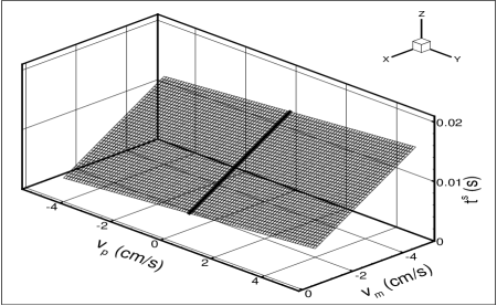
FIG. 8.: The sliding time $t^{s}$ of the particle $i$. The solid line shows the result for a symmetric collision. Here $e_{n}=0.9$ and $C=0.13$.

An interesting effect can be observed in Fig. 9: there is a particular combination of the initial particle velocities that gives vanishing sliding distance. The meaning of this result is that the particle returns to its initial position exactly at the time $t^{s}_{i}$ after the collision; this occurs when ${\bf v}_{i}^{s}=-{\bf v}_{i}^{f}$. Using Eqs. (72, A7), we obtain the condition for zero sliding distance in terms of the initial velocities of the particles

$${\bf v}_{i}^{0}={(e_{n}+2)\left(1+{mR^{2}\over I}\right)+e_{n}{mR^{2}\over I}-2C\over(e_{n}-2)\left(1+{mR^{2}\over I}\right)+e_{n}{mR^{2}\over I}+2C}{\bf v}_{j}^{0}\ .$$ (73)

For a completely elastic collision of solid particles, we obtain ${\bf v}_{i}^{0}=-6{\bf v}_{j}^{0}$. Equation (73) gives clear experimental prediction which can be used to explore how realistic the collision model is.

2 The change of the translational kinetic energy and momentum due to sliding

In this section we give the final results for the change of the translational energy and the linear momentum of the particles due to sliding after a collision. This results assume that the particles slide the whole distance $s$, so that there are no other collisions taking place while the particles travel this distance. Consequently, for a system consisting of many particles (as in [22, 23]), the change of the translational energy due to sliding depends on the distance traveled by the particles in between of the collisions, $l$. When $l$ is on average much larger than the sliding distance, $s$, one could consider modeling the effect of sliding using “effective” coefficient of restitution [22], which we derive below. In this case, we find that this “effective” coefficient of restitution depends only on the usual restitution coefficient, $e_{n}$, and on the geometric properties of the particles. On the other hand, if $l\approx s$, this “effective” coefficient of restitution will depend also on the local density and velocity of the particles. We explore this effect in more details in [25].

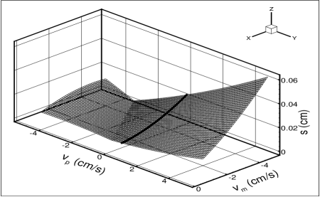
FIG. 9.: The sliding distance s of the particle $i$ ($|{\bf s}_{i}|$ in the text). The solid line shows the result for a symmetric collision ($e_{n}=0.9$ and $C=0.13$).

The change of the translational energy of the particle $i$, $\Delta\bar{E}_{slip}^{i}$, is defined as $\Delta\bar{E}_{slip}^{i}=|{\bf v}_{i}^{f}|^{2}-|{\bf v}_{i}^{s}|^{2}$. The translational velocity of the particle when it stops sliding, ${\bf v}_{i}^{s}$, is given by Eq. (72), and the velocity of the particle at the end of collision, ${\bf v}_{i}^{f}$, is given by Eq. (A7).

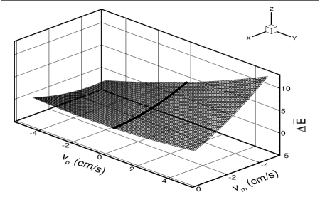
FIG. 10.: The change of the translational energy of the particle $i$ due to sliding ($\Delta\bar{E}_{slip}^{i}$ in the text). The solid line shows the result applicable to symmetric collisions ($e_{n}=0.9$ and $C=0.13$).

Figure 10 shows the results for $\Delta\bar{E}_{slip}^{i}$. We chose to show the total energy change, instead of the relative one, in order to be able to address the case of initially stationary particle, characterized by $E_{0}^{i}=0$. The solid line shows the result for the symmetric case, $v_{p}=0$. From Fig. 10 we observe that the loss of energy of the particle strongly depends on $v_{p}$, i.e. on the degree of the asymmetry of the collision. In particular, we observe that $\Delta\bar{E}_{slip}^{i}$ could attain negative values, meaning that the particle increases its translational kinetic energy due to sliding. In order to illustrate this rather counter-intuitive point, let us consider for a moment completely asymmetric collision, characterized by ${\bf v}_{j}^{0}=v^{0}{\bf\hat{i}}$, ${\bf v}_{i}^{0}=0$. Using Eqs. (72, A7), the change of the energy of the particle $i$ (initially stationary particle), due to sliding, easily follows

$$\Delta\bar{E}_{slip}^{i} ={{1\over 2}(1+e_{n})-C\over\left(1+{mR^{2}\over I}\right)^{2}}\times$$ (75)

$$\left[(1+e_{n})\left({1\over 2}+{mR^{2}\over I}\right)-C\right](v^{0})^{2}\ .$$

Since $C=O(\epsilon)\ll 1$, $\Delta\bar{E}_{slip}^{i}$ is positive, meaning that the particle $i$ loses its translational energy due to sliding after the collision. On the other hand, the change of the energy of the particle $j$ (impact particle), due to sliding, is given by

$$\Delta\bar{E}_{slip}^{j} =-\,{{1\over 2}(1+e_{n})-C\over\left(1+{mR^{2}\over I}\right)^{2}}\times$$ (77)

$$\left[(1-e_{n})\left(1+{mR^{2}\over I}\right)+{1+e_{n}\over 2}-C\right](v^{0})^{2}\ .$$

The negative sign implies that the particle $j$ gains translational energy by sliding. The interpretation of this result is simple, in particular in completely elastic limit, $e_{n}\rightarrow 1$ (also $C\rightarrow 0$). Since the collision is elastic, the translational velocity of the impact particle $j$ vanishes immediately after the collision with the stationary particle $i$. But, the particle $j$ still has the angular velocity, ${\bf\Omega}^{f}_{j}$, which is (in the elastic limit) equal to its initial angular velocity. Consequently, the particle $j$ has the sliding velocity, which is, immediately after the collision, equal to the negative of its initial translational velocity. The sliding acceleration resulting from this sliding velocity induces the motion of the particle in its initial, ${\bf\hat{i}}$, direction. The result is that the translational energy of the particle $j$ is being increased by the action of the friction force between the particle and the substrate after the collision.

Still considering completely asymmetric case, it is of interest to compute the net energy loss of the system of two particles, $\Delta\bar{E}_{slip}^{i,j}=\Delta\bar{E}_{slip}^{i}+\Delta\bar{E}_{slip}^{j}$. By combining Eqs. (75, 77), we obtain

$$\left[\Delta\bar{E}_{slip}^{i,j}\right]^{asymm} ={{1\over 2}(1+e_{n})-C\over\left(1+{mR^{2}\over I}\right)^{2}}\left[(1+e_{n}){mR^{2}\over I}-\right.$$ (79)

$$\left.(1-e_{n})\left(1+{mR^{2}\over I}\right)\right](v^{0})^{2}\ .$$

The net change of the translational energy is positive, as expected, so that the system is losing translational kinetic energy. As in the symmetric case, we obtain the relative loss of energy by dividing with the total initial translational kinetic energy (scaled with reduced mass), $\Delta E_{slip}^{i,j}={\Delta\bar{E}_{slip}^{i,j}/(v^{0})^{2}}$. In the completely elastic case, the result for the relative loss of energy is given by

$$\left[\Delta E_{slip}^{i,j}\right]_{elastic}^{asymm}={2{mR^{2}\over I}\over\left(1+{mR^{2}\over I}\right)^{2}}\ .$$ (80)

Following the same approach, the relative loss of energy of the system of two particles undergoing a symmetric elastic collision (scaled with the total initial energy) is given by (using Eqs. (51, 53))

$$\left[\Delta E_{slip}^{i,j}\right]_{elastic}^{symm}={4{mR^{2}\over I}\over\left(1+{mR^{2}\over I}\right)^{2}}\ .$$ (81)

Comparing Eqs. (80, 81), we see that the particles lose twice as much energy due to sliding in symmetric, compared to completely asymmetric elastic collision. The intuitive understanding of this result follows by realizing that the sliding velocities of the particles at the end of a symmetric collision, scaled by the initial velocities, are larger in the symmetric, compared to the completely asymmetric case (viz. Eq. (67)). The consequence is that the particles that have undergone a symmetric collision slide longer and lose more translational energy. When $C\neq 0$, the loss of energy due to sliding in an inelastic collision is even smaller, since the particle-particle interaction during the collision decreases the angular velocities and, consequently, the sliding velocities of the particles after the collision.

Figure 11 shows the change of momentum due to sliding, defined as $\Delta\bar{p}_{slip}^{i}=({\bf v}_{f}^{i}-{\bf v}_{s}^{i})\cdot{\bf\hat{i}}$, so that it measures the change of the translational velocity of particle $i$ (in the ${\bf\hat{i}}$ direction), after the collision. Clearly, $\Delta\bar{p}_{slip}^{i}$ depends very weakly on the degree of the asymmetry. For completely elastic collisions, $\Delta\bar{p}_{slip}^{i}$ depends only on the relative initial velocity of the particles, and it is given by

$$\left(\Delta\bar{p}_{slip}^{i}\right)_{elastic}=-{1\over 1+{mR^{2}\over I}}({\bf v}_{i}^{0}-{\bf v}_{j}^{0})\cdot{\bf\hat{i}}\ .$$ (82)

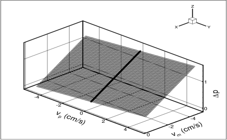
FIG. 11.: The change of the linear momentum of the particle $i$ due to sliding. The solid line shows the result applicable to symmetric collisions ($e_{n}=0.9$ and $C=0.13$).

Effective coefficient of restitution. Let us define $t_{m}$ as the time, measured from the end of a collision, at which neither of the particles slides anymore, so that $t_{m}=max(t_{i}^{s},\,t_{j}^{s})$, where $t_{k}^{s}$ ($k=i,j$) is the sliding time of a particle, given by Eq. (70). We define the effective coefficient of restitution, $e_{n}^{eff}$, as the ratio of the translational velocities of the particles at the time $t_{m}$, and their initial velocities. Using the translational velocity of the particle $i$, given by Eq. (72), and the analogous equation for the particle $j$, we obtain

$$e_{n}^{eff}={|{\bf v}_{i}-{\bf v}_{j}|^{s}\over|{\bf v}_{i}-{\bf v}_{j}|^{0}}={e_{n}{mR^{2}\over I}-1\over 1+{mR^{2}\over I}}\ .$$ (83)

Remarkably enough, this result involves only the “real” coefficient of restitution and the geometric properties of the particles. For solid spheres, the difference between the usual coefficient of restitution and the effective one is huge; for $e_{n}=0.9$, we obtain $e_{n}^{eff}=0.36$. This value is smaller than the range reported in [22], but very close to our experimental results for steel particles on aluminum substrate [24]. Slight imperfections from the spherical shape in experiments, non-central collisions, and/or the fact that the static friction between the particles has been neglected in our calculations, might be the reason for this discrepancy.

General remarks. While more precise analysis and material parameters could be used in order to more precisely model experiments, we consider that the main results and observations given in this section are model-independent. In particular, the observation that the sliding is likely to occur as a consequence of most of the collisions does not depend on the details of the model. Of course, the results would be modified in the case of more complicated (two dimensional) geometry of the collisions. Still, the particular geometry of a collision enters into our results for the energy and momentum change only through the observation that the frictional interaction of the colliding particles with the substrate can be ignored during a collision. Since, for the system that we consider in this work, the collision forces are generally much stronger than the friction forces resulting from particle-substrate interaction, we do not expect this observation to be modified for more complicated collisions. We do note that more realistic model for the particle-particle interactions (e.g. by including static friction) would introduce modifications in the expression for the final angular velocity of the particles, Eq. (66).

In the experiments [22, 23] it is observed that some of the particles travel for long distances without colliding. Especially in this situation, it is important to include the effect of rolling friction, which we have ignored in this section. As long as a particle slides, the effect of rolling friction could be safely neglected, since the coefficient of rolling friction is much smaller than the coefficient of kinematic sliding friction.

V Conclusion

The most important observation made in this work is that sliding leads to a considerable modification of the translational kinetic energy and linear momentum of the particles, even in the limit of completely elastic collisions. Based on this observation we give the result for the “effective” coefficient of restitution, valid for dilute systems, where the mean free path of the particles in between of the collisions is much longer than the sliding distance. For more dense systems, we conjecture that this “effective” coefficient of restitution strongly depends on the local density and velocity of the particles.

The model that we present is to be used in molecular dynamics (MD) type simulations [25] of externally driven system of a set of particles interacting on a horizontally oscillated surface. In particular, we have prepared the grounds for detailed modeling of the system of two kinds of particles, which are characterized by different rolling properties. In [23] is shown that strong segregation can be achieved. Preliminary MD results, based on the model formulated in this paper, show that the realistic modeling of the particle-particle and particle-substrate interactions are needed in order to fully understand this effect.

Further, since experiment is the ultimate test for every theory, it would be of considerable importance to extend the previous work [18, 19, 20, 21] on formulating continuum theory for “2D granular gas”. Using the model presented here should allow for precise comparison between experimental and theoretical results. Possible formulation of realistic continuum, hydrodynamic theory applicable to this seemingly simple system would be an important step towards better understanding of granular materials.

Acknowledgments. The author would like to thank Robert Behringer, David Schaeffer, and in particular Joshua Socolar for useful discussions and comments. This work was supported by NSF Grants No. DMR-9321792 and DMS95-04577, and by ONR Grant No. N00014-96-1-0656.

A Linear model for the normal force between particles

Let us analyze a simple situation, a central collision of two identical particles, $i$ and $j$, moving with the velocities, ${\bf v}_{i}^{0}$ and ${\bf v}_{j}^{0}$, in the ${\bf\hat{i}}$ direction only. Here we ignore the interaction of the particles with the substrate; the importance of this interaction is discussed in Appendix D. Using this assumption, the normal force, given by Eq. (2), is the only force acting on the particle $i$ in the normal direction. By combining the equations of motion for the particles $i$ and $j$, we obtain that the compression depth $x={(d-r_{i,j})/d}$ satisfies the following equation

$$\ddot{x}+\gamma_{N}\dot{x}+\omega_{0}^{2}x=0\ ,$$ (A1)

where $\gamma_{N}$ is the damping coefficient in the normal direction, and $\omega_{0}=\sqrt{2k/m}$. We limit our discussion to the case of low damping, so that $\epsilon={\gamma_{N}/\omega_{0}}\ll 1$.

This equation is subject to the following initial conditions: $x(t=0)=0$, $\dot{x}(t=0)={v^{0}_{rel}/d}$. The relative velocity of the particles at $t=0$ is given by $v^{0}_{rel}=|{\bf v}_{i}^{0}-{\bf v}_{j}^{0}|$; for a symmetric collision, $v^{0}_{rel}=2v^{0}$. The solution is

$$x={v^{0}_{rel}\over d\sqrt{\omega_{0}^{2}-\left({\gamma_{N}\over 2}\right)^{2}}}\exp\left(-{\gamma_{N}\over 2}t\right)\sin\left(\sqrt{\omega_{0}^{2}-\left({\gamma_{N}\over 2}\right)^{2}}t\right)\ .$$ (A2)

The duration of the collision, $t_{col}$, now follows from the requirement $x(t=t_{col})=0$, thus

$$t_{col}={\pi\over\sqrt{\omega_{0}^{2}-\left({\gamma_{N}\over 2}\right)^{2}}}={\pi\over\omega_{0}}(1+O(\epsilon^{2}))\ .$$ (A3)

In what follows, we also need the time of maximum compression, $t_{max}$. From the condition $\dot{x}(t=t_{max})=0$, we obtain

$$\tan\left(\sqrt{\omega_{0}^{2}-\left({\gamma_{N}\over 2}\right)^{2}}t_{max}\right)={\sqrt{\omega_{0}^{2}-\left({\gamma_{N}\over 2}\right)^{2}}\over{\gamma_{N}\over 2}}\ .$$ (A4)

Expanding to $O(\epsilon)$, it follows

$$t_{max}={t_{col}\over 2}\left(1-{\epsilon\over\pi}+O(\epsilon^{2})\right)\ .$$ (A5)

So, the damping manifests itself in a slight asymmetry of the collision, since $t_{max}<{t_{col}/2}$. The maximum compression, $x_{max}=x(t=t_{max})$, follows using Eq. (A2). It is given by Eq. (47) for inelastic collisions, and by Eq. (38) for elastic ones.

We define the coefficient of restitution as the ratio of the final velocities of the particles relative to their initial velocities, i.e. $e_{n}={|{\bf v}_{i}-{\bf v}_{j}|^{f}/|{\bf v}_{i}-{\bf v}_{j}|^{0}}$. It follows

$$e_{n}=-\,{d\over v^{0}_{rel}}\dot{x}(t_{col})=\exp\left({-{\gamma_{N}\over 2}t_{col}}\right)\ =1-{\pi\over 2}\epsilon+O(\epsilon^{2})\ .$$ (A6)

In the limit of low damping, $e_{n}$ is close to $1$; typically we use $e_{n}=0.9$, appropriate for steel particles [22, 23, 24]. Using Eq. (A3), we obtain $\epsilon\approx-{2/\pi}\ln(e_{n})\approx 0.07$.

The final velocity of the particle $i$ (at the end of the collision) follows from the requirement that the total linear momentum is conserved in the center of mass frame. It is given by

$${\bf v}_{i}^{f}={1\over 2}\left[{\bf v}_{i}^{0}+{\bf v}_{j}^{0}-e_{n}({\bf v}_{i}^{0}-{\bf v}_{j}^{0})\right]\ .$$ (A7)

For a symmetric collision, this results simplifies to ${\bf v}_{i}^{f}=-e_{n}{\bf v}_{i}^{0}$.

B Nonlinear models for the normal force between particles

The linear model, presented in the previous section, is the simplest approximation for the collision interaction between particles. Nonlinear terms, resulting from the final area of contact and other effects [31, 32, 38, 42, 43], should be included in order to model the interaction between particles more realistically. Still, since we are concerned with the conditions where the maximum compression depth is small, the linear approximation is a reasonable one. We use the nonlinear model, outlined below, in order to connect the values of the parameters, in particular the collision time, $t_{col}$, with the material properties of the particles.

The general, commonly used equation is [31]

$$\ddot{x}+{\eta d\over m}x^{\gamma}\dot{x}+{Ed\over m}x^{\beta+1}=0\ ,$$ (B1)

where $\eta$ and $E$ are the material constants. The choice $\gamma=0$, $\beta=0.5$ leads to the Hertz model. The analysis of this equation gives an expression for $t_{col}$, that can then be used to determine the appropriate force constant in the linear model, $k$, and the damping coefficient, $\gamma_{N}$. The result for the collision time is [31]

$$t_{col}\approx I(\beta)\left(1+{\beta\over 2}\right)^{1\over 2+\beta}\left({m\over Ed^{1-\beta}}\right)^{1\over 2+\beta}v_{0}^{-{\beta\over 2+\beta}}\ .$$ (B2)

For the Hertz model, $I(0.5)=2.94$. The parameter $E$ is given by ${Y/(3(1-\tilde{\sigma}^{2}))}$, where $Y$ is the Young modulus, and $\tilde{\sigma}$ is the Poisson ratio. We use $Y=2.06\times 10^{12}$ dyn/cm², and $\tilde{\sigma}=0.28$. For steel spheres with diameter $d=4\,$mm, and impact velocity, $v_{0}=10\,$ cm/s, $t_{col}\approx 2.55\times 10^{-5}\,$ sec; for $v_{0}=100\,$ cm/s, $t_{col}\approx 1.61\times 10^{-5}\,$ sec. We note that the model predicts $t_{col}\sim v_{0}^{-1/5}$, and $t_{col}\sim d$. The parameters that enter the linear model can now be calculated, using $\omega_{0}={\pi/t_{col}}(1+O(\epsilon^{2}))$, and $\gamma_{N}=-{2/t_{col}}\ln(e_{n})$.

C Sliding during collisions

1 Sliding during a symmetric collision

In Appendices A and B we obtained the results governing dynamics of particle collisions, ignoring the interaction with the substrate. Here we show that the colliding particles slide through most of a typical collision. The additional material constants that are involved are the coefficients of static and kinematic friction between the considered particles and the substrate, $\mu_{s}$ and $\mu_{k}$. In our estimates, we use $\mu_{s}=0.5$ and $\mu_{k}=0.1$.

The condition for sliding, Eq. (28), applied to the simple situation outlined in section IV A, gives that sliding occurs when $|{\bf F}_{N}^{c}|\geq(1+{mR^{2}/I})\,\mu_{s}mg$. In terms of the compression depth and velocity, this condition is

$$d\omega_{0}^{2}x+d\gamma_{N}\dot{x}\geq\left(1+{mR^{2}\over I}\right)\mu_{s}g\ .$$ (C1)

We note that the left hand side of this equation is always non-negative, since ${\bf F}_{N}^{c}$ is always repulsive (at the very end of a collision, when $x\ll 1$, $\dot{x}<0$, ${\bf F}_{N}^{c}$ is set to $0$). In the limit $\gamma_{N}\rightarrow 0$, we obtain that sliding occurs when $x\geq x_{min}^{0}$, where $x_{min}^{0}=(1+{mR^{2}/I}){\mu_{s}g/(d\omega_{0}^{2})}$. Using the result for the compression depth, Eq. (A2), we obtain the time at which sliding starts, $t_{min}^{0}$, measured from the beginning of the collision,

$$\sin(\omega_{0}t_{min}^{0})=\left(1+{mR^{2}\over I}\right){\mu_{s}g\over v^{0}_{rel}\omega_{0}}\ .$$ (C2)

For the initial velocities, $v^{0}_{rel}$, satisfying $v^{0}_{rel}\gg v^{b}$, where $v^{b}=(1+{mR^{2}/I}){\mu_{s}g/\omega_{0}}$, it follows that $\sin(\omega_{0}t_{min}^{0})\ll 1$. For our set of parameters, and assuming solid spheres, $v^{b}\approx 10^{-2}$ cm/s. Therefore, this condition is satisfied for most of the collisions. Assuming this, we obtain

$$t_{min}^{0}=\left(1+{mR^{2}\over I}\right){\mu_{s}g\over v^{0}_{rel}\omega_{0}^{2}}\ ,$$ (C3)

and

$$x_{min}^{0}=\left(1+{mR^{2}\over I}\right){\mu_{s}g\over d\omega_{0}^{2}}\ .$$ (C4)

Exploiting the symmetry of an elastic collision, we conclude that the sliding condition is satisfied for $t_{min}^{0}<t<t_{col}-t_{min}^{0}$.

Next we go to the limit of small, but finite damping, and assume that the condition $\omega_{0}t_{min}\ll 1$ is still valid, where $t_{min}$ is now the time when sliding occurs for $\gamma_{N}\neq 0$. Using $\gamma_{N}t_{min}\ll\omega_{0}t_{min}$, we Taylor-expand $x$ and $\dot{x}$ (given by Eq. (A2)) at $t=t_{min}$, and keep only the first order terms in small quantities $\omega_{0}t_{min}$, $\gamma_{N}t_{min}$. In this limit,

$$x(t_{min})\approx{v^{0}_{rel}\over d}t_{min};\quad\dot{x}(t_{min})\approx{v^{0}_{rel}\over d}(1-\gamma_{N}t_{min})\ .$$ (C5)

The sliding condition, Eq. (C1), gives the time when sliding occurs, for an inelastic collision

$$t_{min}=\left(1+{mR^{2}\over I}\right){\mu_{s}g\over v^{0}_{rel}\omega_{0}^{2}}-{\epsilon\over\omega_{0}}+O(\epsilon^{2})\ .$$ (C6)

We note that there are two factors that contribute to $t_{min}$: the frictional interaction with the substrate gives the first term on the right hand side of Eq. (C6), and the damping that occurs during a collision gives the second one. For the initial velocities, satisfying $v^{0}_{rel}\gg v^{c}={g\mu_{s}/\gamma_{N}}$, the contribution from the damping is the important one. Using the expression for $\gamma_{N}$ given in Appendix B, we obtain $v^{c}\approx 0.05$ cm/s (for $e_{n}=0.9$). This velocity is smaller than the usual initial velocities considered in this work. Assuming $v^{0}_{rel}\gg v^{c}$, we conclude that the friction term could be relevant only in the limit $e_{n}\rightarrow 1$, since $v^{c}$ diverges in this limit. Consequently, it follows that $t_{min}\rightarrow 0$, so that the sliding starts immediately at the beginning of an inelastic symmetric collision. Since $t_{min}\rightarrow 0$, the expansion used to obtain Eq. (C5) is consistent.

2 Sliding during an asymmetric collision

By combining Eqs. (63, 64), we obtain the condition for sliding during an asymmetric collision

$${\left|{\bf F}_{N,i}^{c}-{mR^{2}\over I}({\bf\hat{k}}\cdot{\bf F}_{R,i}^{c}){\bf\hat{n}}\right|\over 1+{mR^{2}\over I}}\geq\mu_{s}\left|mg-{\bf F}_{R,i}^{c}\cdot{\bf\hat{k}}\right|\ .$$ (C7)

Using Eqs. (2, 65) for ${\bf F}_{N,i}^{c}$ and ${\bf F}_{R,i}^{c}$, respectively, we obtain (in terms of the compression depth, see Appendix A)

$$d\omega_{0}^{2}x+d\gamma_{N}\dot{x}\geq \left(1+{mR^{2}\over I}\right)\mu_{s}g+{\gamma_{S}\over 2}|v_{rel}^{z}|sign(-v_{rel}^{z})\times$$ (C9)

$$\left[{mR^{2}\over I}-\left(1+{mR^{2}\over I}\right)\mu_{s}\right]\ ,$$

where $v_{rel}^{z}$ is given by Eq. (7). From the first part of this Appendix, we already know that the first term on the right hand side is negligible. The term inside the square brackets is positive for solid spheres, and $\mu_{s}=0.5$. For large $x$’s, the condition, Eq. (C9), is always satisfied, since $d\omega_{0}^{2}x$ is the dominant term. So, we need to explore only the beginning and end of a collision. If $sign(-v_{rel}^{z})<0$, the sliding condition is always satisfied; so that the slower particle always slides. When $sign(-v_{rel}^{z})>0$, we concentrate on the very beginning of the collision, and obtain the condition

$$\gamma_{N}\geq{\gamma_{S}\over 2}{|{\bf v}_{i}^{0}+{\bf v}_{j}^{0}|\over|{\bf v}_{i}^{0}-{\bf v}_{j}^{0}|}\left[{mR^{2}\over I}-\left(1+{mR^{2}\over I}\right)\mu_{s}\right]\ .$$ (C10)

Since typically $\gamma_{S}={\gamma_{N}/2}$, this condition is satisfied, assuming $|{\bf v}_{i}^{0}+{\bf v}_{j}^{0}|\approx|{\bf v}_{i}^{0}-{\bf v}_{j}^{0}|$.

We conclude that the particles entering an asymmetric collision slide during the whole course of the collision, except possibly in the case $|{\bf v}_{i}^{0}-{\bf v}_{j}^{0}|\ll|{\bf v}_{i}^{0}+{\bf v}_{j}^{0}|$. We do not consider this case here.

D Modification of collision dynamics due to the interaction with the substrate

Here we estimate the importance of the interaction between the colliding particles and the substrate during a collision. In particular, we estimate under what conditions the interaction with the substrate significantly modifies the results for the compression depth and the duration of a collision. We use the linear model outlined in Appendix A, and concentrate on the case of the particles moving on a horizontal static substrate.

In Appendix C it is shown that, assuming typical experimental conditions, the colliding particles slide relative to the substrate during most of a collision. For simplicity, here we concentrate on a symmetric collision, and further assume that the condition for sliding is satisfied throughout the collision, so that the friction force attains its maximum allowed value, given by Eq. (21). By using this approximation, we slightly overestimate the influence of the friction with the substrate on the dynamics of a collision.

From Fig. 4 we observe that the friction force, $\bf f$, acts in the direction opposite to the normal collision force, ${\bf F}_{N}^{c}$. Including $\bf f$ in the Newton equations of motion for the particles $i$ and $j$, we obtain the modified equation for the compression depth

$$\ddot{x}+\gamma_{N}\dot{x}+\omega_{0}^{2}x-\mu_{k}{g\over d}=0\ ,$$ (D1)

which simplifies to Eq. (A1) if the particle-substrate interaction is ignored.

Using the initial conditions as in Appendix A, we obtain the solution

$$x=x_{f}-\exp\left(-{\gamma_{N}\over 2}t\right)\left[x_{f}\cos\left(\sqrt{\omega_{0}^{2}-\left({\gamma_{N}\over 2}\right)^{2}}t\right)-\right.$$ (D2)

$$\left.{{v^{0}_{rel}\over d}-{1\over 2}x_{f}\gamma_{N}\over\sqrt{\omega_{0}^{2}-\left({\gamma_{N}\over 2}\right)^{2}}}\sin\left(\sqrt{\omega_{0}^{2}-\left({\gamma_{N}\over 2}\right)^{2}}t\right)\right]\ ,$$ (D3)

where $x_{f}={\mu_{k}g/(d\omega_{0}^{2}})$.

Collision time. For simplicity, we concentrate on the case of zero damping ($\gamma_{N}=0$), and calculate the change of the duration of the collision due to the particle-substrate interaction. Let us assume that the change of the collision time is small, and write $t_{col}^{\prime}=t_{col}+\tau$, where $t_{col}={\pi/\omega_{0}}$ is the collision time if there is no interaction with the substrate, and $\tau\ll t_{col}$. Using the condition $x(t=t_{col}^{\prime})=0$, and expanding the compression depth, given by Eq. (D3), to the first order in the small quantity $\tau\omega_{0}$, we obtain that $\tau={2x_{f}d/v^{0}_{rel}}$. So, the relative change of the collision time due to the interaction with the substrate is given by

$${t_{col}^{\prime}-t_{col}\over t_{col}}={2\mu_{k}g\over\pi v^{0}_{rel}\omega_{0}}\ .$$ (D4)

For $v^{0}_{rel}\gg v^{a}$, where $v^{a}\approx{\mu_{k}g/\omega_{0}}$, the change of the collision time is small. Using the parameters given in Appendices B and C, we estimate $v^{a}\approx 10^{-3}$ cm/s. So, for most of the experimentally realizable conditions, the duration of a collision is just very weakly influenced by the particle-substrate interaction. We assume $v^{0}_{rel}\gg v^{a}$, so that $\tau\omega_{0}\ll 1$, and the expansion of Eq. (D3) is consistent.

Maximum compression depth. Following the same approach, we estimate the modification of the maximum compression achieved during a collision, due to the interaction with the substrate. Working in the limit of zero damping, and assuming a small modification of the time, $t_{max}$, when the maximum compression, $x_{max}^{\prime}$, is reached, we obtain $x_{max}^{\prime}\approx x_{f}+{v^{0}_{rel}/(d\omega_{0})}$. Comparing this result with the result for the compression depth calculated previously, given by the elastic limit of Eq. (47), we obtain

$${x_{max}^{\prime}-x_{max}\over x_{max}}=d\omega_{0}{x_{f}\over v^{0}_{rel}}={\mu_{k}g\over v^{0}_{rel}\omega_{0}}\ .$$ (D5)

Similarly to the analysis of the collision time, we observe that for $v^{0}_{rel}\gg v^{a}$, the maximum compression depth is very weakly influenced by the particle-substrate interaction.

We conclude that for most of collisions occurring in experiments, the interaction with the substrate just slightly modifies the compression depth and the duration of a collision. These small modifications are ignored in the subsequent analysis.

E Rotations of the particles during a collision

1 Rotations during symmetric collisions

During symmetric collisions, the rotational motion of the particles is influenced only by the friction force between the particles and the substrate. Here we consider only elastic collisions, since in Appendix C it is shown that the particles entering an inelastic collisions start sliding immediately, so that the angular acceleration is constant during the whole course of collision, simplifying the calculations (see section IV A 2). Since there is no possibility of confusion, we use scalar notation, with the sign convention that +sign corresponds to the forces acting in $+{\bf\hat{i}}$ direction, and to the angular motion in $+{\bf\hat{j}}$ direction (the coordinate axes are as shown in Fig. 4).

At the very beginning of an elastic collision, for $0<t<t_{min}^{0}$, ($t_{min}^{0}$ is given by Eq. (C3)), the colliding particles do not slide. During this time interval, the angular acceleration of the particle $i$, which initially moves in $-{\bf\hat{i}}$ direction, is given by

$$\dot{\Omega}_{i}={R\over I}f_{i}={R\over I}{F_{N,\,i}^{c}\over 1+{mR^{2}\over I}}={{mR\over I}\over 1+{mR^{2}\over I}}v^{0}_{rel}\omega_{0}^{2}t\ ,$$ (E1)

where $x\approx t{v^{0}_{rel}/d}$, and Eqs. (2, 37) have been used. Integration yields

$$\Omega_{i}(t=t_{min}^{0})=\Omega_{i}^{0}+{1\over 2}{mR\over I}\left(1+{mR^{2}\over I}\right){(\mu_{s}g)^{2}\over v^{0}_{rel}\omega_{0}^{2}}\ ,$$ (E2)

and $\Omega_{i}^{0}=-{v^{0}/R}$. For $t_{min}^{0}<t<t_{col}-t_{min}^{0}$, the sliding condition, $|{\bf f}_{i}|=\mu_{s}|{\bf F}_{N,\,i}^{c}|$, is satisfied, so that the angular acceleration reaches its maximum (constant) value

$$\dot{\Omega}_{i}={mR\over I}\mu_{k}g\ .$$ (E3)

For $t_{col}>t>t_{col}-t_{min}^{0}$, the sliding condition is not satisfied anymore, but the particle is sliding already, so that $\dot{\Omega}_{i}$ is still given by Eq. (E3). The angular velocity of the particle $i$ at the end of collision is

$$\Omega_{i}^{f0}=\Omega_{i}(t=t_{min}^{0})+{mR\over I}\mu_{k}g(t_{col}-t_{min}^{0})\ .$$ (E4)

Combining Eqs. (E2, E4), we obtain the final result, given by Eq. (43).

2 Rotations during asymmetric collisions

a About tangential force

Here we estimate under what conditions, ${\bf F}_{R}^{c}$, given by Eq. (6), reaches its maximum allowed value, $\nu_{k}|{\bf F}_{N}^{c}|$. As mentioned in section IV B, here we ignore the frictional interaction of the particles with the substrate during a collision. For simplicity, we also neglect the damping in the normal directions, so that $|{\bf F}_{N}^{c}|=md\omega_{0}^{2}x$ (see Appendix A). Next, we note that the relative velocity of the point of contact satisfies $v_{rel}^{z}(t=0)>v_{rel}^{z}(t>0)$, since ${\bf F}_{R}^{c}$ always decreases $v_{rel}^{z}$ (given by Eq. (7)). In what follows, we use $v_{rel}^{z}(t>0)=v_{rel}^{z}(t=0)$, and give the upper limit of the first term entering the definition of ${\bf F}_{R}^{c}$.

Let us first concentrate on large compression depths, $x\approx x_{max}={|{\bf v}_{i}^{0}-{\bf v}_{j}^{0}|/(d\omega_{0})}$ (see Appendix A). This compression is reached at $t=t_{max}={\pi/(2\omega_{0})}$. We use $v_{rel}^{z}(t=t_{max})=v_{rel}^{z}(t=0)=|{\bf v}_{i}^{0}+{\bf v}_{j}^{0}|$, and obtain that ${\bf F}_{R}^{c}$ reaches its maximum allowed value if (see Eq. (6))

$${\gamma_{S}\over 2}|{\bf v}_{i}^{0}+{\bf v}_{j}^{0}|\geq\nu_{k}\omega_{0}|{\bf v}_{i}^{0}-{\bf v}_{j}^{0}|\ .$$ (E5)

Since ${\gamma_{S}/\omega_{0}}\ll 1$, this condition is never satisfied for $\nu_{k}=O(1)$, and $|{\bf v}_{i}^{0}+{\bf v}_{j}^{0}|\approx|{\bf v}_{i}^{0}-{\bf v}_{j}^{0}|$.

For small $x$’s, let us assume again $v_{rel}^{z}(t>0)=v_{rel}^{z}(t=0)$. From Eq. (6) it follows that ${\bf F}_{R}^{c}$ reaches its cutoff value when $x<x^{crit}$, where

$${x^{crit}\over x_{max}}={\gamma_{S}\over 2\nu_{k}\omega_{0}}{|{\bf v}_{i}^{0}+{\bf v}_{j}^{0}|\over|{\bf v}_{i}^{0}-{\bf v}_{j}^{0}|}=O(\epsilon)\ .$$ (E6)

Using $x\approx{t|{\bf v}_{i}^{0}-{\bf v}_{j}^{0}|/d}$ (valid for $x\ll x_{max}$), we obtain that the condition $x<x^{crit}$ is satisfied for $t<t^{crit}$, where

$${t^{crit}\over t_{max}}={\gamma_{S}\over\pi\omega_{0}}{|{\bf v}_{i}^{0}+{\bf v}_{j}^{0}|\over|{\bf v}_{i}^{0}-{\bf v}_{j}^{0}|}=O(\epsilon)\ .$$ (E7)

In order to calculate the angular velocity of the particle $i$ at the end of a collision, ${\bf\Omega}_{i}^{f}$, we have to integrate the angular acceleration, ${\bf\dot{\Omega}}_{i}$, during the course of a collision. The angular acceleration is proportional to ${\bf F}_{R}^{c}$, as it follows from Eq. (59), where ${\bf f}_{i}$ is being neglected. In performing the integration, it appears that we have to consider separately two regions: $0<t<t^{crit}$, during which ${\bf F}_{R}^{c}$ varies, and $t>t^{crit}$, during which ${\bf F}_{R}^{c}$ is constant. The final angular velocity of the particle $i$ is formally given by

$${\bf\Omega}_{i}^{f}={\bf\Omega}_{i}^{0}+\int_{0}^{t^{crit}}{\bf\dot{\Omega}}_{i}dt+\int_{t^{crit}}^{t_{col}}{\bf\dot{\Omega}}_{i}dt\ .$$ (E8)

This result can be simplified by realizing that $|{\bf F}_{R}^{c}|=O(\epsilon)$. It follows that $|{\bf\dot{\Omega}}_{i}|=O(\epsilon)$, so that the contribution of the second term on the right hand side of Eq. (E8) is proportional to $|{\bf\dot{\Omega}}_{i}|t^{crit}=O(\epsilon^{2})$. For consistency reasons we neglect this correction, and ignore the fact that $|{\bf F}_{R}^{c}|$ could reach Coulomb cutoff at the very beginning and end of a collision. This estimate is not valid for $|{\bf v}_{i}^{0}-{\bf v}_{j}^{0}|\ll|{\bf v}_{i}^{0}+{\bf v}_{j}^{0}|$, so when the particles initially move with almost the same velocities. As already mentioned in Appendix C, we do not consider this case here.

b The angular velocity of the particles during an asymmetric collision

Using Eqs. (59, 65), and neglecting the particle-substrate interaction during a collision, we obtain the angular acceleration of the particle $i$,

$${\bf\dot{\Omega}}_{i}=-\,{mR^{2}\over I}{\gamma_{S}\over 2}[({\bf\Omega}_{i}+{\bf\Omega}_{j})\cdot{\bf\hat{j}}]\ {\bf\hat{j}}\ ,$$ (E9)

and ${\bf\dot{\Omega}}_{j}={\bf\dot{\Omega}}_{i}$. Recalling that ${\bf\dot{\Omega}}_{i}$ and ${\bf\dot{\Omega}}_{j}$ are always in the opposite direction from ${\bf\Omega}_{i}+{\bf\Omega}_{j}$, we obtain a simple system of coupled ordinary differential equations

$${\bf\dot{\Omega}}_{i}=-\,C^{\prime}({\bf\Omega}_{i}+{\bf\Omega}_{j})\ ,$$ (E10)

$${\bf\dot{\Omega}}_{j}=-\,C^{\prime}({\bf\Omega}_{i}+{\bf\Omega}_{j})\ ,$$ (E11)

where $C^{\prime}={mR^{2}\gamma_{S}/(2I)}$. We define ${\bf\Omega}_{+}={\bf\Omega}_{i}+{\bf\Omega}_{j}$, so that ${\bf\dot{\Omega}}_{+}=-\,2C^{\prime}{\bf\Omega}_{+}$, with the solution

$${\bf\Omega}_{+}(t)={\bf\Omega}_{+}(t=0)\exp(-2C^{\prime}t)\ .$$ (E12)

At $t=t_{col}$, ${\bf\Omega}_{+}(t=t_{col})={\bf\Omega}_{+}(t=0)\exp(-2C)$, where $C=C^{\prime}\,t_{col}=O(\epsilon)$. Recalling that the changes of ${\bf\Omega}_{i}$ and ${\bf\Omega}_{j}$ are the same, so that ${\bf\Omega}_{k}(t=t_{col})={\bf\Omega}_{k}(t=0)+\Delta{\bf\Omega}$, ($k=i,j$), the change of the angular velocities is given by

$$\Delta{\bf\Omega}={1\over 2}\left[({\bf\Omega}_{i}^{0}+{\bf\Omega}_{j}^{0})(\exp(-2C)-1)\right]\approx-({\bf\Omega}_{i}^{0}+{\bf\Omega}_{j}^{0})C\ ,$$ (E13)

correct to the first order in $\epsilon$. For $\gamma_{S}={\gamma_{N}/2}$, and the parameters as in Appendix B, $C={\pi mR^{2}\epsilon/(4I)}\approx 0.13$. The final angular velocity of the particle $i$ is now given by Eq. (66).

F Jump condition for asymmetric particle collisions

Throughout this work, we have assumed that the particles are bound to move on the surface of the substrate. Here we explore the validity of this assumption. The required condition for a particle to be bound to the substrate is that the normal force $|{\bf F}_{N}|$, given by Eq. (64), is nonzero. We immediately observe that only a particle colliding with a slower particle (so that $sign(-v_{rel}^{z})<0$, see Eq. (7)) experiences a force in $+{\bf\hat{k}}$ direction, due to a collision. Let us concentrate on this situation. Using the value of $|{\bf F}_{R}^{c}|$ at $t=0$, we obtain that a particle detaches from the substrate if

$$f_{net}=m\left({\gamma_{S}\over 2}|v_{rel}^{z}|-g\right)>0\ ,$$ (F1)

where Eqs. (7, 64, 65) have been used. It follows that, during the collisions distinguished by $|v_{rel}^{z}|>v^{d}={2g/\gamma_{S}}$, the faster particle detaches from the substrate. Using the values of the parameters as in Appendix B, and $\gamma_{S}={\gamma_{N}/2}$, we obtain $v^{d}\approx 0.5$ cm/s. Correspondingly, this effect takes place during most of the asymmetric collisions occurring in typical experiments [22, 23]. By relating the impulse of the force $f_{net}$ transferred to a particle while the collision is taking place, with the change of the momentum of the particle in the ${\bf\hat{k}}$ direction, we obtain the estimate for the initial velocity of the particle in the ${\bf\hat{k}}$ direction

$$v^{z}=\left({\gamma_{S}\over 2}|v_{rel}^{z}|-g\right){\pi\over\omega_{0}}\ .$$ (F2)

The maximum height above the substrate which the particle reaches is $h^{z}={1/2}{(v^{z})^{2}/g}$, and the time spent without contact with the substrate is $t^{z}={2v^{z}/g}$. Let us assume a completely asymmetric collision, so that $|{\bf v}_{i}^{0}|=v^{0}$, $|{\bf v}_{j}^{0}|=0$, and $v_{rel}=v_{rel}^{z}=v^{0}$. Using the parameters from Appendix B, for $v^{0}=10$ cm/s, we obtain $v^{z}\approx 0.5$ cm/s, $h^{z}\approx 1.3\times 10^{-4}$ cm, and $t^{z}\approx 10^{-2}$ sec. Since the maximum height is much smaller than the diameter of the particles, this detachment introduces negligible corrections to the dynamics of the particle collisions in $x-y$ plane. Further, even though $t^{z}\gg t_{col}$, so that the particle is not in the contact with the substrate during the time which is much longer than the duration of the collision, $t^{z}$ is still much smaller then the sliding time scale, specified by Eq. (70). So, our results for sliding of the particles after a collision are not significantly modified due to the detachment effect.

REFERENCES

- [1] E-mail: kondic@math.duke.edu
- [2] E. Rabinowicz, Friction and Wear of Materials, (Wiley, New York, 1965).
- [3] F. Heslot, T. Baumberger, B. Perin, B. Caroli, and C. Caroli, Phys. Rev. E 49, 4973 (1994).
- [4] O. Raynolds, Phil. Trans. R. Soc. London 166, 155 (1876).
- [5] D. Tabor, Proc. R. Soc. London A 229, 198 (1955).
- [6] J. A. Greeenwood, H. Minshall, and D. Tabor, Proc. R. Soc. London A 259, 480 (1961).
- [7] K. N. G. Fuller and A. D. Roberts, J. Phys. D 14, 221 (1981).
- [8] N. V. Brilliantov and T. Pöschel, Europhys. Lett. 42, 511 (1998).
- [9] A. Domenech, T. Domenech, and J. Cebrian, Am. J. Phys. 55, 231 (1987).
- [10] R. Ehrlich and J. Tuszynski, Am. J. Phys. 63, 351 (1995).
- [11] J. Gersten, H. Soodak, and M. S. Tiersten, Am. J. Phys. 60, 43 (1992).
- [12] B. Bernu and R. Mazighi, J. Phys. A 23, 5745 (1990).
- [13] S. McNamara and W. R. Young, Phys. Fluids A 4, 496 (1992); ibid 5, 34 (1993).
- [14] N. Sela and I. Goldhirsch, Phys. Fluids 7, 507 (1995).
- [15] E. L. Grossman and B. Roman, Phys. Fluids. 8, 3218 (1996).
- [16] P. Constantin, E. Grossman, and M. Mungan, Physica D 83, 409 (1995).
- [17] Y. Du, H. Li, and L. P. Kadanoff, Phys. Rev. Lett. 74, 1268 (1995).
- [18] S. McNamara and W. R. Young, Phys. Rev. E 50, 28 (1994).
- [19] S. McNamara and W. R. Young, Phys. Rev. E 53, 5089 (1996).
- [20] I. Goldhirsch and G. Zanetti, Phys. Rev. Lett. 70, 1619 (1993).
- [21] E. L. Grossman, T. Zhou, and E. Ben-Naim, Phys. Rev. E 55, 4200 (1997).
- [22] A. Kudrolli, M. Wolpert, and J. P. Gollub, Phys. Rev. Lett. 78, 1383 (1997).
- [23] S. Tennakoon and R. P. Behringer, in preparation.
- [24] B. Painter, L. Kondic, S. Tennakoon, and R. P. Behringer, in preparation.
- [25] L. Kondic, S. Tennakoon, and R. P. Behringer, in preparation.
- [26] H. M Jaeger, S. R. Nagel, and R. P. Behringer, Rev. Mod. Phys. 68, 1259 (1996).
- [27] P. K. Haff and B. T. Werner, Powder Technology 48, 239 (1986).
- [28] C. S. Campbel and C. E. Brennen, J. Fluid Mech. 151, 167 (1985).
- [29] H. J. Herrmann, in Disorder and Granular Media, Ed. D. Bideau and A. Hansen, (North-Holland, Amsterdam) (1993).
- [30] P. A. Thompson and G. S. Grest, Phys. Rev. Lett. 67, 1751 (1991).
- [31] S. Luding, E. Clement, A. Blumen, J. Rajchenbach, and J. Duran, Phys. Rev. E 50, 4113 (1994).
- [32] G. H. Ristow, J. Phys. I (France) 2, 649 (1992).
- [33] P. K. Haff, in Granular Matter, Ed. A. Mehta, (Springer-Verlag, New York) (1994).
- [34] P. A. Cundall and O. D. L. Strack, Géotechnique 29, 47 (1979).
- [35] O. R. Walton and R. L. Braun, J. Rheol. 30, 949 (1986).
- [36] K. Walton, J. Mech. Phys. Solids 35, 213 (1987).
- [37] J. D. Goddard, Proc. R. Soc. London 430, 105 (1990).
- [38] Y. Taguchi, J. Phys. II France, 2, 2103 (1992).
- [39] F. Radaji and S. Roux, Phys. Rev. E 51, 6177 (1995).
- [40] F. Radaji, L. Brendel, and S. Roux, Phys. Rev. E 54, 861 (1996).
- [41] F. Radaji, P. Evesque, D. Bideau, and S. Roux, Phys. Rev. E 52, 5555 (1995).
- [42] N. V. Brilliantov, F. Spahn, J. Hertzsch, and T. Pöschel, Phys. Rev. E 53, 5382 (1996).
- [43] T. Schwager and T. Pöschel, Phys. Rev. E 57, 650 (1998).
- [44] C. M. Dury and G. H. Ristow, to be published.