Abstract

These are notes for lectures delivered at the NATO ASI on Dynamics in Leiden, The Netherlands, in July 1998. The main concepts relating to quantum phase transitions are explained, using the paramagnet-to-ferromagnet transition of itinerant electrons as the primary example. Some aspects of metal-insulator transitions are also briefly discussed. The exposition is strictly pedagogical in nature, with no ambitions with respect to completeness or going into technical details. The goal of the lectures is to provide a bridge between textbooks on classical critical phenomena and the current literature on quantum phase transitions. Some familiarity with the concepts of classical phase transitions is helpful, but not absolutely necessary.

Contribution to: Dynamics: Models and Kinetic Methods for Non-

equilibrium Many-Body Systems

John Karkheck (editor)

To be published by Kluwer academic publishers b.v.

Lectures delivered by D. Belitz

1 Introduction to Continuous Phase Transitions

In these lectures we discuss so-called quantum phase transitions or zero-temperature phase transitions. Our motivation is the fact that these transitions provide a field where the long-range correlations in quantum systems that were introduced in the preceding lectures [1] have some spectacular consequences. Since quantum phase transitions have many features in common with ordinary classical or thermal phase transitions, we will first review the basic concepts of both, and then define and discuss the particular features of quantum transitions, before turning to some specific examples. We would like to warn the reader that it is not possible to do this subject justice within the time and space constraints of these lectures. Our aim can therefore only be to give some examples that highlight a few of the interesting features of the field. Thorough treatments of the phenomenology and theory of classical phase transitions can be found in Refs. [2], and aspects of quantum phase transitions are reviewed in Refs. [3, 4].

1.1 Review of basic concepts

Continuous phase transitions

Continuous phase transitions are characterized by the system under consideration undergoing a transition from a symmetric or disordered state, which incorporates some symmetry of the Hamiltonian, to a broken-symmetry or ordered state, which does not have that symmtry, although the Hamiltonian still possesses it. A good example is given by a Heisenberg ferromagnet: The relevant symmetry of the Hamiltonian is the rotational symmetry in spin space, and the disordered and ordered states are represented by the paramagnetic and the ferromagnetic states, respectively. In the former, there is no preferred direction for the magnetic moments of the spins. The net magnetization is therefore zero, and the state has the same spin rotational symmetry as the Hamiltonian. That is, if we rotate the coordinate system in spin space, then the system will look the same. In the latter, on the other hand, there is a preferred direction for the spins, and this is the direction which the overall magnetization will point in. The state therefore does no longer respect the spin rotational symmetry, and we say that the symmetry is spontaneously broken (‘spontaneously’, in order to distinguish this phenomenon from the explicit or external breaking that occurs if we apply an external magnetic field). In an ideal system the preferred direction is completely arbitrary, and in real systems it is determined by very small external fields, like e.g. the earth’s magnetic field, or by a small breaking of the symmetry in the system’s Hamiltonian as provided by, e.g., the ionic lattice strucuture. As a result, in an ideal system the magnetization in the ordered state is not only non-zero, but it is also non-unique. Such a thermodynamic quantitity that is zero in the disordered phase, and non-zero and non-unique in the ordered phase, is called an order parameter, a concept first introduced by Landau. The external field $B$ that couples to the order parameter, in our example the magnetic field, is called the field conjugate to the order parameter.

As we approach the phase transition by changing some parameter, several remarkable phenomena are observed. For instance, the correlations of the order parameter become long-ranged. Let $M$ be the order parameter, and let us consider the spatial correlations of $M$ (in the case of a magnet, they can be measured by neutron scattering):

$$\langle M({\bf x})\,M({\bf y})\rangle=f(|{\bf x}-{\bf y}|/\xi)\quad.$$ (1)

Everywhere in parameter space except at the critical point, the function $f$ decays in space on a length scale $\xi$ called the correlation length. $\xi$ diverges as the critical point is approached, usually like a power law that is characterized by the correlation length critical exponent, $\nu$:

$$\xi\propto t^{-\nu}\quad,$$ (2)

where $t$ denotes some dimensionless distance in parameter space from the critical point. For instance, if the transition occurs at a non-zero critical temperature $T_{\rm c}$, we can use $t=|T-T_{\rm c}|/T_{\rm c}$. At criticality, i.e. at $t=0$, the correlation length diverges, which indicates that the order parameter correlations decay only like a power law, which has no intrinsic scale. It is customary to denote this power law by an exponent $\eta$:

$$\langle M({\bf x})\,M({\bf y})\rangle_{t=0}\propto|{\bf x}-{\bf y}|^{-d-2+\eta}\quad,$$ (3)

where $d$ denotes the spatial dimensionality of the system.

Apart from these long-range correlations in space, there are similar effects in the temporal behavior of the system. Let us denote the equilibration time, i.e. the time scale for the system to return to equilibrium after it has been disturbed, by $\tau_{c}$. This equilibration time diverges as criticality is approached, and it does so as a power of the correlation length, with the power law characterized by an exponent $z$:

$$\tau_{c}\propto\xi^{z}\quad,$$ (4)

The inverse of $\tau_{c}$ defines a critical frequency scale $\omega_{c}$ that goes to zero as criticality is approached, a phenomenon called critical slowing down:

$$\omega_{c}(t\rightarrow 0)\propto 1/\tau_{c}\rightarrow 0\quad.$$ (5)

The exponents $\nu$, $\eta$, and $z$ that we have defined so far are examples of critical exponents, which characterize the power law behavior of various observables upon approach to the critical point. Three other important critical exponents are $\beta$, which describes the vanishing of the order parameter,

$$M(t\rightarrow 0)\propto t^{\beta}\quad,$$ (6)

$\gamma$, which describes the diverges of the order parameter susceptibility, which in our example is the magnetic susceptibility $\chi=M/B$,

$$\chi(t\rightarrow 0)\propto t^{-\gamma}\quad,$$ (7)

and the critical exponent $\delta$, which describes the dependence of the order parameter on its conjugate field at criticality,

$$M(t=0,B\rightarrow 0)\propto B^{1/\delta}\quad,$$ (8)

Notice that a diverging susceptibility implies that there cannot be a region where the order parameter depends linearly on the conjugate field.

The set of critical exponents characterizes the critical behavior, and it turns out that all of the critical exponents are not independent. Rather, many of them are related to one another by scaling laws or exponent relations. Furthermore, it turns out that the complete set of critical exponents is the same for whole classes of phase transitions. For instance, the critical exponents for the ferromagnetic transitions in iron and nickel are the same, even though these three metals have very different bandstructures, and their Curie temperatures are very different. Perhaps even more surprisingly, the critical exponents observed at the critical point of water are the same as those at the liquid-gas critical points of the “quantum liquids” He3 and He4. Phase transitions that share the same critical behavior, as expressed by the critical exponents, are said to belong to the same universality class, and the existence of such universality classes is referred to as universality or universal behavior. It turns out that universality classes are determined by basic symmetries of the underlying Hamiltonian, and by the spatial dimensionality of the system. The fact that the critical behavior is independent of the microscopic details of the Hamiltonian is due to the diverging correlation length: Close to a critical point, the system performs an average over all length scales that are smaller than the (very large) correlation length. This observation also gives a clue as to how to theoretically deal with critical phenomena: In order to correctly describe the universal critical behavior it should be sufficient to work with an effective theory that keeps explicitly only the asymptotic long-wavelength or large-distance behavior of the original Hamiltonian. By contrast, observables that vary from system to system even within a given unversality class, like e.g. the critical temperature, are called non-universal properties, and they are not accessible by means of such effective theories.

The theoretical understanding of these, and other, properties of phase transitions took place over a period of 100 years, starting with van der Waals, continuing with Landau, and ending with Wilson. Wilson’s renormalization group, the essence of which is a set of scale transformations, provided us with a deep understanding of the origin of universality and the critical power laws. More recently, it has also turned out to be a very useful general tool for studying the statistical mechanics of many-body systems in general, not only close to some critical point. Here it is not our goal to describe the renormalization group, for this purpose we refer the reader to the many excellent expositions in the literature [5]. Rather, we will take the critical phenomenology for granted, and on its basis discuss the role of quantum mechanics in the context of phase transitions. The only exception is Sec. 2.3, where we assume some familiarity with basic renormalization group arguments in order to derive some results. As an explicit example, we will stick to ferromagnets, except in Sec. 3 which deals with metal-insulator transitions.

1.2 Classical versus quantum phase transitions

A fundamental question is the following: To what extent is quantum mechanics necessary in order to understand the critical phenomena we have sketched in the previous subsection, and to what extent will classical physics suffice? One can get the correct answer by means of the following very simple considerations (which can be elaborated upon if that is considered desirable). Generally speaking, quantum mechanics is important whenever the temperature becomes lower than some characteristic energy of the system under consideration. For instance, in an atom that characteristic energy is the Rydberg energy. In our case, we have seen that there is a characteristic frequency, namely $\omega_{c}$. Let us assume that the corresponding energy scale, $\hbar\omega_{c}$, is the smallest relevant energy scale. Since $\omega_{c}(t\rightarrow 0)\rightarrow 0$, this is a reasonable guess close to the transition. It then follows that quantum mechanics will be important whenever the temperature $T$ obeys

$$k_{\rm B}T<\hbar\omega_{c}\quad.$$ (9)

Usually we think of phase transitions as taking place at some non-zero critical temperature $T_{c}$, e.g. at the Curie temperature in our magnetic example. It then follows that sufficiently close to the transition, namely for

$$t<(T_{c}/T_{0})^{1/\nu z}\quad,$$ (10)

we expect quantum mechanics not to be important for describing the system’s behavior. Here $T_{0}$ is some microscopic temperature scale, e.g., the Fermi temperature in a metallic ferromagnet. It follows that for any phase transition that takes place at a non-zero critical temperature $T_{c}>0$, the critical behavior asymptotically close to the transition can be described entirely by classical physics. This conclusion survives more rigorous arguments. These phase transitions are called classical or thermal transitions. What drives the correlation length to infinity are thermal fluctuation, which become very large close to criticality. In contrast, we might think of a transition that occurs at zero temperature, and that is triggered by varying some non-thermal parameter, e.g. the system’s composition. For instance, if $n$ is the concentration of some ingredient, and $n_{\rm c}$ is the critical concentration, we can choose $t=|n_{\rm c}-n|/n_{\rm c}$ as our dimensionless distance from criticality. Then it obviously follows that quantum mechanics will be important for describing the critical behavior. These transitions are called quantum or zero-temperature phase transitions, and the relevant fluctuatations are quantum fluctuations or zero-point motion. An example would be a magnetic system that is, at $T=0$, continuously diluted with some non-magnetic material until it undergoes a transition to the paramagnetic state. (We will deal with the obviously relevant question of what happens at low, but non-zero, temperatures in the following subsection.) Notice that, according to this definition, some phase transitions in systems that are usually considered quintessentially quantum mechanical, like the superconducting transition in mercury at $T=4.2\,{\rm K}$, or the $\lambda$-transition in helium at $T=2.17\,{\rm K}$, are classical transitions. Indeed, in both cases the critical behavior (but not the physics that triggers the transition, or the properties of either phase) can be understood entirely by means of classical physics: Both transitions are in the universality class of a classical 3-d xy-model.

Classical phase transitions

Let us now first consider some additional properties of classical phase transitions. Within classical statistical mechanics, consider a Hamiltonian

$$H(p,q)=K(p)+U(q)\quad,$$ (11)

where $p$ and $q$ are the generalized momenta and positions, and $K$ and $U$ are the kinetic and potential energy, respectively. The partition function

$$Z=\int dp\,dq\ e^{-H/k_{\rm B}T}=\int dp\ e^{-K/k_{\rm B}T}\int dq\ e^{-U/k_{\rm B}T}\quad,$$ (12)

then factorizes into a piece that depends only on $K$ and one that depends only on $U$. As a result, one can study the system’s static properties independently from its dynamical ones. In particular, the dynamical critical exponent $z$ is independent from all of the other critical exponents, and the static critical behavior can be studied, following Landau, by means of an effective functional of a time-independent order parameter. One often expresses this by saying that ‘statics and dynamics decouple’.

Close to the critical point, the free energy density, $f=(-1/V)\,k_{\rm B}T\,\ln Z$, obeys a generalized homogeneity law,

$$f(t,B,\ldots)=b^{-d}\,f(t\,b^{1/\nu},B\,b^{x_{B}},\ldots)\quad.$$ (13)

Here $V$ is the system volume, and $t$ and $B$ are the dimensionless distance from the critical point and the external field conjugate to the order parameter, respectively, as before. $b$ is an arbitrary positive real number called a scale parameter, and Eq. (13) holds for all $b>0$. $\nu$ is the correlation length critical exponent, and $x_{B}>0$ is a critical exponent that is related to $\delta$ by $x_{B}=d\delta/(1+\delta)$. Since all thermodynamic quantities can be obtained from the free energy, Eq. (13) provides us with homogeneity laws for all of them. For instance, by differentiating $f$ with respect to $B$ we obtain a homogeneity law for the order parameter density, $M=\partial f/\partial B$,

$$M(t,B)=b^{x_{B}-d}\,M(t\,b^{1/\nu},B\,b^{x_{B}})\quad.$$ (14)

Since $b$ is arbitrary, we can in particular put $b=B^{-1/x_{B}}$. At $t=0$ we then recover the above relation between $x_{B}$ and $\delta$. By the same method, other exponent relations can be obtained, and it turns out that of all the static critical exponents, only two are independent, e.g. $\nu$ and $x_{B}$. Another useful substitution is to set $b=t^{-\nu}\propto\xi$. This makes it obvious that letting $b\rightarrow\infty$ is tantamount to approaching criticality. In this context, a remark about the suppressed variables in Eq. (13), which we denoted by “$\ldots$”, is in order. They all enter Eq. (13) analogously to $t$ and $B$, but the exponents that characterize their ‘scaled’ entries on the right-hand side (i.e. the analogs of $1/\nu$ and $x_{B}$), turn out to be negative. As a result, these entries go to zero as one approaches criticality, and are called ‘irrelevant variables’ or ‘irrelevant operators’. If the observable under consideration is a regular function of a particular variable for small values of the argument, then it follows that this variable becomes unimportant as we approach criticality and does not influence the critical behavior. It thus really becomes ‘irrelevant’ in the ordinary sense of the word. This is not the case, however, if the observable is a singular function of some argument for small values of the argument. In this case the irrelevant variable influences the critical behavior after all, and one speaks of a ‘dangerous irrelevant variable’. Dangerous irrelevant variables can cause substantial complications in the technical analysis of scaling near critical points.

The homogeneity or scaling law, Eq. (13), was historically first postulated phenomenologically, and it turned out that all observed properties of phase transitions followed from it if appropriate values for $\nu$ and $x_{B}$ were used, depending on the universality class under consideration. It was the triumph of Wilson’s renormalization [6] group that it allowed a derivation of the homogeneity law from first principles. This derivation is highly technical, and we cannot go into it. Instead, we refer the reader to the extensive literature on this subject [5].

Quantum phase transitions

Let us now turn to the case of quantum phase transitions, i.e. transitions that occur at $T=0$ and are triggered by some non-thermal control parameter. As we have seen above, in this case quantum mechanics is always important, and we need to employ quantum statistical mechanics in order to calculate the partition function and the free energy. Let the Hamilton operator of the system be ${\hat{H}}({\hat{a}}^{\dagger},{\hat{a}})$, with ${\hat{a}}^{\dagger}$ and ${\hat{a}}$ a collection of creation and annihilation operators. In the usual imaginary time formalism, the time evolution of ${\hat{a}}$ is given by ${\hat{a}}({\tau})=e^{{\hat{H}}\tau}\,{\hat{a}}\,e^{-{\hat{H}}\tau}$, with $\tau$ the imaginary time variable. A general theorem [7] then tells us that the partition function for any quantum many-body system can be written as a function integral of the form

$$Z=\int D[{\bar{\psi}},\psi]\ e^{S[{\bar{\psi}},\psi]}\quad.$$ (15)

Here ${\bar{\psi}}$ and $\psi$ are space and imaginary time dependent fields that are isomorphic to the sets of creation and annihilation operators in a second quantization formulation of the problem. Their nature depends on whether the quantum particles are fermions or bosons: For the latter, the fields are classical or bosonic (i.e., they commute), while for the former, they are fermionic (i.e., they anticommute). $D[{\bar{\psi}},{\psi}]$ is an appropriate integration measure defined with respect to these fields [8]. The action $S[{\bar{\psi}},\psi]$ is uniquely determined by the Hamilton operator, and is given by

$$S[{\bar{\psi}},{\psi}] = \int d{\bf x}\int_{0}^{1/k_{\rm B}T}d\tau\ {\bar{\psi}}({\bf x},\tau)\,\left[-\frac{\partial}{\partial\tau}+\mu\right]\,\psi({\bf x},\tau)$$ (16)

$$-\int_{0}^{1/k_{\rm B}T}d\tau\ H\left({\bar{\psi}}({\bf x},\tau),\psi({\bf x},\tau)\right)\quad.$$

Here $H$ as a function of ${\bar{\psi}}$ and $\psi$ has the same functional form as ${\hat{H}}$ as a function of ${\hat{a}}^{\dagger}$ and ${\hat{a}}$.

Since the Hamiltonian taken at some imaginary time does not commute with the Hamiltonian taken at another imaginary time, we see that for quantum systems the statics and the dynamics are intrinsically coupled and need to be treated together and simultaneously. All phenomena that need to be described by means of quantum statistical mechanics, and quantum phase transitions in particular, therefore automatically fall under the title of this NATO ASI. It further follows that for quantum phase transitions, in contrast to classical ones, there are three independent critical exponents, and the dynamical exponent $z$ needs to be determined together with the static ones.

The homogeneity law for the free energy density, Eq. (13), can now easily be generalized to the quantum case. From Eqs. (2) and (4,5) we see that, as a function of $t$, frequencies scale like $t^{\nu z}$. Furthermore, in the imaginary time formalism, temperature and Matsubara frequencies are directly proportional to one another, and it is therefore plausible that temperature and frequency will scale in the same way. We thus add $T$ as an argument to our free energy density and acknowledge the explicit $T$ in the definition of $f$ to obtain

$$f(t,T,B,\ldots)=b^{-(d+z)}\,f(t\,b^{1/\nu},T\,b^{z},B\,b^{x_{B}},\ldots)\quad.$$ (17)

Comparing Eqs. (13) and (17) we see that a quantum phase transition in $d$ spatial dimensions resembles the corresponding classical transition in $d_{\rm eff}=d+z$ spatial dimensions! This is also plausible from the point of view of the Landau functional (see below), where a spatial integral $\int d{\bf x}$ in the classical case gets replaced by a space-time integral $\int d{\bf x}\,d\tau$ in the quantum case. Early work on the subject suggested that this observation provides a fast and easy solution to the problem of quantum critical behavior. However, as we will see, the argument is too superficial to be reliable, and the extent to which it holds requires a careful and detailed discussion.

1.3 An example: The paramagnet-to-ferromagnet transition

Let us illustrate the concepts introduced above by means of a concrete example. For definiteness, we consider a metallic or itinerant ferromagnet.

The phase diagram

Figure 1 shows a schematic phase diagram in the $T$-$J$ plane,

Figure 1.  : Schematic phase diagram showing a paramagnetic (PM) and a ferromagnetic (FM) phase. The path indicated by the dashed line path represents a classical phase transition, and the one indicated by the solid line a quantum phase transition.

with $J$ the strength of the exchance coupling that is responsible for ferromagnetism. The coexistence curve separates the paramagnetic phase at large $T$ and small $J$ from the ferromagnetic one at small $T$ and large $J$. For a given $J$, there is a critical temperature, the Curie temperature $T_{\rm c}$, where the phase transition occurs. This is the usual situation: A particular material has a given value of $J$, and the classical transition is triggered by lowering the temperature through $T_{\rm c}$. Alternatively, however, we can image changing $J$ at zero temperature (e.g. by alloying the magnet with some non-magnetic material). Then we will encounter the paramagnet-to-ferromagnet transition at the critical value $J_{\rm c}$. This is the quantum phase transition we are interested in. Since we have seen that the quantum transition is, loosely speaking, related to the classical one in a different spatial dimensionality, and since we know that changing the dimensionality usually means changing the universality class, we expect the critical behavior at this quantum critical point to be different from the one observed at any other point on the coexistence curve.

This brings us to the question of how continuity is guaranteed when one moves along the coexistence curve. The answer, which was found by Suzuki [9], also explains why the behavior at the $T=0$ critical point is relevant for observations at small but non-zero temperatures. Consider Fig. 2, which shows an enlarged

Figure 2.  : Schematic phase diagram as in Fig. 1 showing the vicinity of the quantum critical point $(J=J_{\rm c},T=0)$. Indicated are the critical region, and the regions dominated by the classical and quantum mechanical critical behavior, respectively. A measurement along the path shown will observe the crossover from quantum critical behavior away from the transition to classical critical behavior asymptotically close to it.

section of the phase diagram near the quantum critical point. The critical region, i.e. the region in parameter space where the critical power laws can be observed, is bounded by the two dashed lines. It then turns out that the critical region is divided into two subregions, denoted by ‘QM’ and ‘classical’ in Fig. 2, in which the observed critical behavior is predominantly quantum mechanical and classical, respectively. The division between these two regions (shown as a dotted line in Fig. 2) is not sharp (and neither is the boundary of the critical region), but rather a smooth crossover from predominantly quantum mechanical to predominantly classical critical behavior is observed as $J$ is increased at low but non-zero $T$. The figure illustrates that the asymptotic critical behavior, very close to the transition, is classical for all non-zero $T$, but that for small $T$ there nevertheless is a sizeable region where quantum critical behavior is observable. It also makes it clear that the abovementioned continuity is realized by means of a distribution limit.

Classic results for itinerant ferromagnets

The subject of quantum magnetic phase transitions was pioneered by Hertz [10], who built on earlier work by Suzuki [9] and others [11]. Hertz’s main result can be recovered by combining the above observation that the quantum phase transition should correspond to the classical one in $d_{\rm eff}=d+z$ dimensions, with the fact that for classical magnets the upper critical dimension $d_{\rm c}^{+}$, i.e. the dimensionality above which the critical behavior is mean-field like, is $d_{\rm c}^{+}=4$. It then follows that for the quantum transition, $d_{\rm c}^{+}=4-z$. Hertz further found that $z=3$ for clean itinerant ferromagnets, and $z=4$ for disordered ones (we will reproduce his results in Sec. 2 below). It then seemed to follow that $d_{\rm c}^{+}=1$ for clean magnets, and $d_{\rm c}^{+}=0$ for disordered ones, so that the quantum critical behavior would be mean-field like in all physical dimensions ($d=2,3$).

These classic results, which seemed to solve the problem (albeit the answer was not very interesting from a theoretical point of view), cannot be correct, however, since they violate other, very general results that were obtained around the same time. Curiously, this contradiction went unnoticed for more than 20 years.

In 1974, Harris [12] argued that at any critical point in a system that contains quenched disorder, the correlation length exponent must obey the inequality

$$\nu\geq 2/d\quad,$$ (18)

in order for the critical behavior to be stable with respect to the disorder. Harris’ physical arguments were later augmented by Chayes et al. [13], who proved a rigorous mathematical theorem to the same effect. Now the mean-field value of $\nu$ is $\nu_{\rm MF}=1/2$, which violates Harris’ criterion for all $d<4$. Hence Hertz’s results for disordered systems cannot be correct. It was also pointed out by Sachdev [14] that Hertz’s results for clean systems in $d<1$ (an academic, but nonetheless interesting case) were at odds with some general scaling arguments.

It finally turned out that the classic results for both the clean and the disordered case are indeed incorrect, for rather subtle and interesting reasons. It also was shown that the theory can be salvaged with relatively little effort, provided that one acknowledges the long-range correlations in itinerant electron systems that were explained in the preceding lectures [1]. This theory was developed in a series of papers [15], the main arguments and results of which we reproduce in the next section.

2 Quantum Critical Behavior of Itinerant Ferromagnets

We now sketch the derivation of an effective field theory for itinerant ferromagnets, starting from a microscopic Hamiltonian. As we will see, the derivation makes massive use of our knowledge of the properties of non-magnetic electron systems. It is this knowledge that makes the task of determining the correct quantum critical behavior much easier than it would have been in the 1970s.

2.1 Landau-Ginzburg-Wilson theory

Let us consider a microscopic model for an itinerant ferromagnet. What we have in mind is to develop an effective theory from such a miscroscopic model that will be capable of correctly describing the quantum critical behavior without being more detailed than necessary in other respects. To this end we follow Landau’s strategy [17] of formulating a theory in terms of an appropriate order parameter, and integrating out all other degrees of freedom. For a ferromagnet, the relevant observable is the spin density

$${\bf n}_{\rm s}({\bf x},\tau)={\bar{\psi}}({\bf x},\tau)\,{\vec{\sigma}}\,\psi({\bf x},\tau)\quad,$$ (19)

where the vector $\vec{\sigma}$ denotes the Pauli matrices. The relevant electron-electron interaction is the spin-triplet interaction between the spin density fluctuations,

$$S_{\rm int}=J\int d{\bf x}\int_{0}^{1/k_{\rm B}T}d\tau\ {\bf n}_{\rm s}({\bf x},\tau)\,\cdot\,{\bf n}_{\rm s}({\bf x},\tau)\quad.$$ (20)

The complete action is

$$S=S_{\rm 0}+S_{\rm int}\quad.$$ (21)

Here $S_{\rm 0}$ comprises all parts of the action other than $S_{\rm int}$ as defined in Eq. (20): It contains a term describing free electrons (or lattice electrons) as well as electron-electron interactions in all channels other than the spin-triplet one. In particular, $S_{\rm 0}$ contains the direct or Coulomb interaction between the electronic charge densities. We will refer to the fictitious system that is described by the action $S_{\rm 0}$ as the reference ensemble, and it will play an important role in what follows.

Our goal is to calculate the partition function

$$Z=\int D[{\bar{\psi}},\psi]\ e^{S_{\rm 0}[{\bar{\psi}},\psi]}\,e^{J\int dx\ {\bf n}_{\rm s}(x)\cdot{\bf n}_{\rm s}(x)}\quad.$$ (22)

Here and it what follows we adopt a four-vector notation $x\equiv({\bf x},\tau)$ for space-time integrals. We now concentrate on the term $S_{\rm int}$, and decouple it by means of a Gaussian or Hubbard-Stratonovich transformation [18]. The latter consists of introducing a classical (i.e. commuting) auxiliary field $M(x)$ that couples linearly to the spin density, and rewriting $e^{S_{\rm int}}$ as a Gaussian integral,

$$Z=\int D[{\bar{\psi}},\psi]\ e^{S_{\rm 0}[{\bar{\psi}},\psi]}\,\int D[M]\ e^{-J\int dx\ M^{2}(x)+2J\int dx\ M(x)n_{\rm s}(x)}\quad.$$ (23)

From now on, for simplicity we ignore the vector nature of the spin density. Taking it into account just complicates the notation without leading to qualitatively important effects. Next, we interchange the $M$ and $\psi$-integrations, and formally carry out the latter,

$$Z=\int D[M]\ e^{-J\int dx\ M^{2}(x)}\ Z_{\rm 0}[M]\quad,$$ (24)

where we recognize

$$Z_{\rm 0}[M]=\int D[{\bar{\psi}},\psi]\ e^{S_{\rm 0}[{\bar{\psi}},\psi]+2J\int dx\ M(x)\,n_{\rm s}(x)}\quad,$$ (25)

as the partition function of the reference ensemble in an external ‘magnetic field’ that is proportional to $M(x)$. From the linear coupling between $M(x)$ and the spin density it is clear that the expectation values of these two quantities are proportional to one another. We thus identify $M(x)$ as the order parameter field whose expectation value is the magnetization. It is customary to define a Landau-Ginzburg-Wilson or LGW functional $\Phi[M]$,

$$\Phi[M]=J\int dx\ M^{2}(x)-\ln Z_{\rm 0}[M]\quad,$$ (26)

where

$$Z_{\rm 0}[M]=\langle e^{2J\int dx\ M(x)\,n_{\rm s}(x)}\rangle_{\rm 0}\quad.$$ (27)

Here $\langle\ldots\rangle_{\rm 0}$ denotes an average with respect to the reference ensemble action $S_{\rm 0}$, and the partition function can be expressed in terms of the LGW functional as

$$Z=\int D[M]\ e^{-\Phi[M]}\quad.$$ (28)

The above derivation of an order parameter theory for quantum ferromagets is due to Hertz [10]. The salient point is that the LGW functional is given in terms of the free energy of the reference ensemble in a (space and time dependent) ‘external field’ that is given by the order parameter field. A more technical way to say this is that the LGW is given by the generating functional for connected spin density correlation functions in the reference ensemble, viz. $\ln Z_{\rm 0}$. Notice that all of the above have been exact manipulations. The strategy underlying this exact rewriting of the partition function is to express the free energy of the full system, which undergoes a phase transition, in terms of that of the reference ensemble, which does not. The price one pays is that one needs to know the free energy of the latter in the presence of an arbitrary space and time dependent magnetic field. As we will see, however, enough is known about correlated electrons in magnetic fields to successfully implement this strategy.

2.2 The Landau expansion

Follwing Landau, the next step is to expand the LGW functional in powers of $M$. Remembering that the reference ensemble has no spontaneous magnetization, and hence $\langle n_{\rm s}\rangle_{0}=0$, we have

$$Z_{\rm 0}=1+2J^{2}\int dx\,dy\ M(x)\,M(y)\,\langle n_{\rm s}(x)\,n_{\rm s}(y)\rangle_{\rm 0}+\ldots\quad,$$ (29)

where the terms not shown explicitly are of $O(M^{4})$ or higher. Taking a Fourier transform, we thus obtain for the LGW functional

$$\Phi[M] = \frac{1}{V}\sum_{\bf q}T\sum_{\omega}M({\bf q},\omega)\,\left[1-J\chi_{\rm s}(q,\omega)\right]\,M(-{\bf q},\omega)$$ (30)

$$\qquad+\sum_{\{{\bf q},\omega\}}u_{4}(\{{\bf q},\omega\})\,M^{4}({\bf q},\omega)+\ldots\quad,$$

where $q=|{\bf q}|$, and

$$\chi_{\rm s}(q,\omega)=\langle n_{\rm s}({\bf q},\omega)\,n_{\rm s}(-{\bf q},-\omega)\rangle_{0}^{\rm c}\quad,$$ (31)

is the connected two-point spin-density correlation function of the reference ensemble, i.e., its spin susceptibility,

$$u_{4}=\langle n_{\rm s}\,n_{\rm s}\,n_{\rm s}\,n_{\rm s}\rangle_{0}^{\rm c}\quad,$$ (32)

is the corresponding connected four-point function, etc. We have used an obvious schematic notation for the quartic terms, since we will not study them in detail here.

The salient point of this formal development is that the LGW functional is given in terms of the connected spin density correlation functions of the reference ensemble. The reference ensemble, however, is a Fermi liquid, or its generalization to the case of quenched disorder, and so its correlation functions are known! Indeed, the preceding lectures [1] has explained in some detail what they are, and we can now draw on that knowledge. For the sake of definiteness we will discuss only disordered systems, where the effects we want to demonstrate are most pronounced. Qualitatively similar, albeit weaker, phenomena are present in clean systems as well, as has been discusssed in the original literature [15]. The appropriate limit to study the correlation functions is that of small wavenumbers and frequencies, $q,\omega\rightarrow 0$, with $\omega\ll q$ in suitable units. As we have seen in the preceding lectures [1, 20] the spin susceptibility of a disordered Fermi liquid in this limit reads

$$\chi_{\rm s}(q,\omega)=\chi_{\rm s}^{0}(q)\,\left[1-|\omega|/Dq^{2}+\ldots\right]\quad,$$ (33)

and the long-wavelength expansion of the static spin susceptibility $\chi_{\rm s}^{0}$ reads

$$\chi_{\rm s}^{0}(q)={\rm const.}-q^{d-2}-q^{2}+o(q^{2})\quad,$$ (34)

where $o(q^{2})$ denotes terms that are smaller than $q^{2}$, and we have omitted positive prefactors of all terms in the expansion, as they will not be important for what follows. The LGW functional now takes the form

$$\Phi[M] = \frac{1}{V}\sum_{\bf q}T\sum_{\omega}M({\bf q},\omega)\,\left[t+q^{d-2}+q^{2}+|\omega|/q^{2}\right]\,M(-{\bf q},-\omega)$$ (35)

$$\qquad\qquad\qquad\qquad\qquad+O(M^{4})\quad.$$

The four-point correlation function $u_{4}$ also contains nonanalyticities, which show up the in the quartic term in $\Phi[M]$, and the same is true for all higher order terms. While a careful study of these terms is necessary for a complete treatment of the problem, we suppress them here for brevity and simplicity, and refer the interested reader to the original literature where they have been discussed in detail [15].

Before we analyze the LGW functional, Eq. (35), in the next subsection, two remarks are in order. First, if we had used a reference ensemble of non-interacting electrons, rather than our more realistic one that includes electron-electron interactions, then we would have missed the non-analytic terms proportional to $q^{d-2}$ in Eqs. (34) and (35). As a consequence, we would have recovered Hertz’s results which, as we have seen earlier, cannot be correct. While it seems at this point as if a realistic choice of the reference ensemble were crucial, this is disturbing from some fundamental theoretical points of view. Indeed, a careful investigation reveals that the precise choice of the reference ensemble is not important. We will come back to this point in Sec. 2.4 below. Second, the physical origins of the $q^{d-2}$ term are long-range spatial correlations in the reference ensemble of interacting electrons that underlies our effective LGW action, as has been explained in the preceding lectures [1]. These long-range spatial correlations are in turn a consequence of the coupling of statics and dynamics in quantum systems. We now see what has happened: In addition to the order parameter fluctuations that develop a long range near criticality, our electron systems also contains long-range correlated degrees of freedom (viz. the ‘diffusons’ of the preceding lectures) that have nothing to do with phase transition physics, and that are present even far away from the transition. These degrees of freedom have been integrated out in our derivation of the LGW functional, which by definition is a functional of the order parameter field only. The inevitable consequence of this integrating out of slow modes is nonanalyticities in the resulting LGW functional. Such nonanlyticities violate the very spirit of the LGW concept, and to perform explicit calculations for the non-local field theory given by Eq. (35) would be very difficult indeed. An obvious way to avoid these problems would be to not integrate out the diffusons, but rather derive a generalized LGW theory in terms of all the soft modes in the systems. However, as we will see in the next subsection, for the purpose of determining the critical behavior the non-local theory can be handled, and the present route is the fastest one to answer the questions we have asked.

2.3 Renormalization group analysis

To finish our treatment of itinerant ferromagnets, we now analyze the LGW functional, Eq. (35), by means of power counting or a tree-level renormalization group (RG) analysis. Space and time constraints do not allow us to explain this technique here. Readers not familiar with it can find excellent and very accessible treatments in Refs. [2].

Let us restrict ourselves to spatial dimensions $d<4$, where the $q^{d-2}$ term dominates over the analytic $q^{2}$ term, and let us look for a Gaussian RG fixed point where neither the $q^{d-2}$ term nor the $|\omega|/q^{2}$ term in Eq. (35) are renormalized. At such a fixed point, the critical order parameter correlation function will behave like

$$\langle M\,M\rangle_{t=0}\propto 1/q^{d-2}\equiv q^{2-\eta}\quad,$$

where the last relation reflects the definition of the critical exponent $\eta$, see Eq. (3). We thus have

$$\eta=4-d\quad.$$ (36)

Furthermore, at such a Gaussian fixed point the frequency clearly scales with the wavenumber like $\omega\sim q^{d}\equiv q^{z}$, which yield a dynamical critical exponent

$$z=d\quad.$$ (37)

Finally, the exponent $\gamma$ for the Gaussian fixed point can also just be read off the Gaussian action: At zero frequency and wavenumber, we have

$$\langle M\,M\rangle_{q=\omega=0}\propto 1/t\equiv t^{-\gamma}\quad,$$

so that we have

$$\gamma=1\quad.$$ (38)

In order to determine the correlation length exponent $\nu$, we define the scale dimension $[q]$ of a wavenumber $q$ to be $[q]=1$. The requirement that the $q^{d-2}$ term in the LGW functional be dimensionless then leads to a scale dimension of the order parameter field of $[M]=-(d-2)/2$. Since the $t$ term must also be dimensionless, this yields

$$t\sim q^{d-2}\sim\xi^{-(d-2)}\equiv\xi^{-1/\nu}\quad,$$

from which we read off $\nu$ as

$$\nu=1/(d-2)\quad.$$ (39)

All of these results obviously hold only for $2<d<4$. For $d\leq 2$ the electrons in the reference ensemble become localized (see the preceding lectures) and our theoretical framework breaks down, while for $d>4$ the $q^{2}$ term dominates over the $q^{d-2}$ term, and we recover Hertz’s mean-field exponents, i.e. $\eta=0$, $z=4$, $\gamma=1$, and $\nu=1/2$.

A quick check shows that our result fulfils the Harris criterion, $\nu\geq 2/d$ (see Sec. 1.3 above) for all values of $d$. While this is encouraging, it is of course only a necessary criterion for our results representing the correct quantum critical behavior, not a sufficient one. To establish the latter, one needs to consider the higher order terms in the LGW functional, and establish that our Gaussian fixed point is stable. At tree level, this has been done in the original literature [15], and the result was that the fixed point is indeed stable. The analysis of the quartic term in $\Phi$ in particular also yields the equation of state, and thus the critical behavior of the order parameter itself, i.e. the critical exponents $\beta$ and $\delta$. The result is

$$\beta=2/(d-2)\qquad,\qquad\delta=d/2\quad,$$ (40)

for $2<d<6$, while for all $d>6$ these exponents have their mean-field values $\beta=1/2$ and $\delta=3$, respectively. The analysis of the higher order terms thus establishes $d=6$ as another upper critical dimensionality, in addition to $d=4$. In $d=4$ and in $d=6$ logarithmic corrections to scaling occur, as is usually the case at an upper critical dimensionality.

Finally, we mention again that an analogous analysis of clean systems yields qualitatively very similar results. Essentially, the exponent $d-2$ in the non-analytic terms gets replaced by $d-1$, which leads to a single upper critical dimension $d_{\rm c}^{+}=3$. Contrary to the disordered case, the critical behavior in the most interesting dimension $d=3$ is therefore mean-field like with logarithmic corrections to scaling [15].

2.4 Final remarks

We finish this section with a few additional remarks. As we have sketched in the preceding subsection, and as has been more carefully established in the original literature, we have managed to determine the critical behavior at the quantum ferromagnetic transition exactly, yet this behavior is not mean-field like. This is surprising, as usually non-mean field like critical behavior cannot be obtained exactly, save for a very few models. To find out what has enabled us to do so, let us look again at our LGW functional, Eq. (35). One way to state the effect of the non-critical soft modes that have led to the $q^{d-2}$ term is to say that they have established an effective long-range interaction between the order parameter fluctuations. Indeed, a Fourier transform of the non-analytic term yields an interaction that falls off like $1/r^{2(d-1)}$. It is well known that such long-range interactions stabilize Gaussian critical behavior that is not mean-field like [21]. What is remarkable here is that this long-range interaction is not put in by hand, but rather is generated by the system itself via the non-critical slow modes.

These considerations raise the question of whether the phenomenon discussed here is germane to quantum phase transitions. In principle, it is not. Whenever there are slow modes in addition to the order parameter fluctuations that couple to the latter, one will obtain nonanalyticities in the LGW functional, and resulting unusual critical behavior, irrespective of whether one deals with a classical or a quantum phase transition. However, quantum transitions are much more susceptible to this mechanism, for the simple reason that there are many modes that are soft only at $T=0$ and acquire a mass at non-zero temperature. Our diffusons are a good example: As was discussed in the preceding lectures, they are indeed massive at $T>0$.

Finally, we come back to a point raised at the end of Sec. 2.2. There we mentioned that whether or not one obtains the correct critical behavior seems to depend crucially on the choice of the reference ensemble. While one might argue that a non-interacting reference ensemble is simple not a realistic model, this leads to the following paradox: Suppose we consider a model whose action consists only of a free electron part, and the spin-triplet interaction $S_{\rm int}$ of Eq. (20). Then a decoupling of $S_{\rm int}$, as performed above, seems to lead to mean-field critical behavior. However, if we considered some fraction of $S_{\rm int}$ a part of $S_{0}$, and decoupled the rest, then we would have an interacting reference ensemble and would obtain the above non-mean field like critical behavior. Clearly, both procedures are equally valid and should lead to the same result. The resolution of this paradox is as follows. In the case of an interacting reference ensemble, already the bare LGW functional contains the crucial nonanalyticities. Therefore, a RG analysis at tree level is sufficient to obtain the correct critical behavior. In the case of a non-interacting reference ensemble, on the other hand, the bare action does not contain the crucial non-analytic terms, but they are generated if the RG analysis is carried to higher order in the loop expansion. Indeed, an inspection of Hertz’s model shows that the $q^{d-2}$ term is indeed generated by the RG, starting at one-loop order. Since the generated term is relevant with respect to the mean-field fixed point, it invalidates the zero-loop analysis. These observations serve as a reminder of a fact that is well-known in principle, but occasionally forgotten: Any RG analysis to a given order in a loop expansion gives the correct answer only if no relevant new terms in the action are generated at higher order. Unfortunately, proving that no such terms are generated at any order in the loop expansion amounts to proving that the theory is renormalizable, a task that is very difficult and has been done only for a few select models.

3 The Anderson-Mott Transition

At the end of these lectures, we would like to briefly touch upon some very different quantum phase transitions, namely the types of metal-insulator transition known as Anderson, and Anderson-Mott transitions, respectively. Our motivation for doing so is chiefly to dispel any possible misconception that the concepts developed so far apply only to quantum phase transitions that are magnetic in nature, or that are represented as the $T=0$ end point of a line of classical phase transitions. Indeed, the Anderson-Mott transition is neither. We would also like to illustrate the point that the scaling ideas that have been so successful in connection with phase transitions, classical and quantum mechanical, may be applied to transport coefficients as well as to thermodynamic quantities [22]. Apart from making these two point, the time and space we devote to this subject are grossly inadequate. Extensive reviews can be found in Refs. [23, 3, 24, 25].

3.1 The simplest metal-insulator transition: The classical Lorentz model

The simplest metal-insulator transition occurs in a classical model, viz. the classical Lorentz gas. It is well known that with increasing scatterer density $n$, the diffusivity $D$ of the moving particle decreases (see the preceding lectures), until if finally reaches zero at a critical scatterer density $n_{\rm c}$. This behavior can be seen in the numerical data shown in Fig. 3.

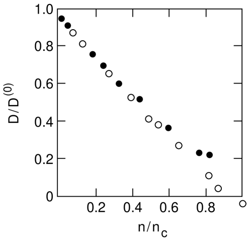
Figure 3.  : Numerical simulation data for the diffusion coefficient $D$ versus the scatterer density $n$ of a $2$-$d$ classical Lorentz model. Full symbols represent data by Bruin [30], and open ones data by Alder and Alley[31], and by Alley[32]. $D$ is normalized by its Boltzmann value $D^{(0)}$, and $n$ by its critical value $n_{\rm c}$. From Ref. [23].

With $t=|n-n_{\rm c}|/n_{\rm c}$ the dimensionless distance from the critical point, one has

$$D(t\rightarrow 0)\propto t^{s}\quad,$$ (41)

with $s$ a critical exponent. The reason for the localization of the diffusing particle is that with increasing scatterer density it is increasingly likely to get trapped in cages of scatterers from which it cannot escape.

3.2 Electrons: The Anderson transition, and the Mott transition

Let us now add quantum mechanics to these considerations, and consider the quantum Lorentz model that was discussed in detail in the preceding lectures. Quantum mechanics has two competing effects on the transport properties: On the one hand, it should increase the diffusivity, since it allows the particle to tunnel out of cages it would be trapped in classically. On the other hand, it leads to the quantum interference or weak-localization effects that enhance the backscattering amplitude. As we saw in the preceding lectures, the latter effect wins. The quantum Lorentz model therefore has a stronger tendency to localize the particle than the classical one, to the point that in $d=2$ the particle is localized even for arbitrarily small scatterer density. In $d>2$, however, there is a metal-insulator transition at a finite value of $n$, which is called an Anderson transition.

The Anderson transition is a strange phase transition from a statistical mechanics point of view, as it has no simple order parameter, and no upper critical dimensionality. However, it has a lower critical dimensionality, $d_{\rm c}^{-}=2$, as for $d\leq 2$ there is no transition. This has been exploited for studies of the Anderson transition in $\epsilon=d-2$ expansions. More generally, the dynamical conductivity $\sigma$ (or, alternatively, the diffusion coefficient $D$) obeys a generalized homogeneity law [26]

$$\sigma(t,\omega)=b^{-(d-2)}\,\sigma(t\,b^{1/\nu},\omega\,b^{z})\quad.$$ (42)

Putting $\omega=0$, and $b=t^{-\nu}$, we obtain from Eq. (42) the behavior of the static conductivity,

$$\sigma(t,0)\propto t^{s}\quad,$$ (43)

with a conductivity exponent

$$s=\nu(d-2)\geq 2(d-2)/d\quad.$$ (44)

The equality in Eq. (44) is known as Wegner’s scaling law, and the inequality results from the Harris criterion, Eq. (18). Due to the poor convergence properties of the $2+\epsilon$ expansions, no reliable theoretical values for $s$ or $\nu$ are available. Numerical calculations in $d=3$ yield values for $\nu$ in the range 1.3 - 1.5 [25].

The quantum Lorentz model does not contain any electron-electron interaction, and the Anderson transition is therefore entirely driven by disorder. The opposite case, namely a metal-insulator transition that is entirely driven by interactions, with no quenched disorder present, was proposed by Mott to explain why certain materials with one electron per unit cell, e.g. NiO, are insulators. Mott’s original idea hinged on the long-range nature of the Coulomb interaction, and in this case the metal-insulator transition comes about by means of a breakdown of screening and is of first order [27]. A similar, albeit continuous, transition is believed to occur in a model with a short-ranged electron-electron interaction known as the Hubbard model. This Mott-Hubbard transition is still not well understood in $d=3$, although much progress has been made recently on high-dimensional models [28].

3.3 The Anderson-Mott transition

An Anderson-Mott transition results if one combines the driving forces for the Anderson and Mott transitions and considers the case of interacting electrons in the presence of disorder. This is a problem of great experimental interest. For instance, the metal-insulator transition that is observed in doped semiconductors as a function of the dopant concentration is believed to be of that type. Fig. 4

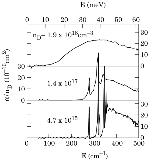
Figure 4.  : Infrared absorption coefficient $\alpha$ for three different donor concentrations $n_{\rm D}$ in Si:P as measured by Thomas at al. [33]. The critical concentration in this system is $n_{\rm c}\approx 3.7\times 10^{18}\,{\rm cm}^{-3}$. From Ref. [23].

shows the infrared absorption spectrum of phosphorus-doped silicon. For very low dopant concentrations one sees a hydrogen-like spectrum that is produced by isolated phosphorus atoms. With increasing dopant concentration these ‘atoms’ start to overlap, which leads to a broadening of the spectral features. At the highest concentration shown in the figure, the spectrum is smooth, but it still represents an insulator (no absorption at zero energy). With further increasing donor concentration, the system undergoes a quantum phase transition to a metal, as can be seen in Fig. 5,

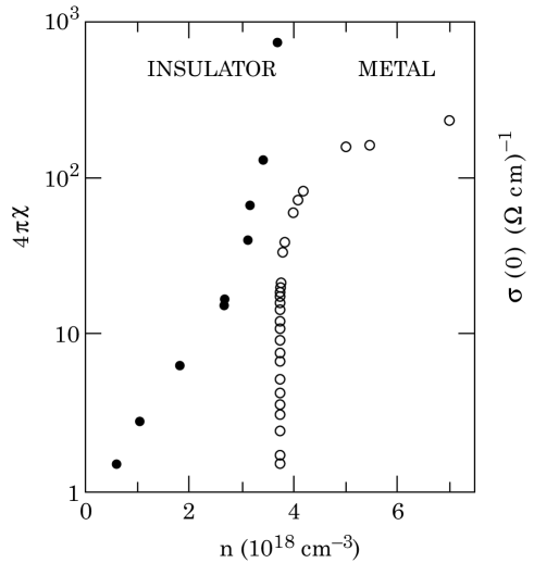
Figure 5.  : Divergence of the dielectric susceptibility $\chi$ (full symbols), and vanishing of the static conductivity $\sigma$ (open symbols), both extrapolated to zero temperature, at the metal-insulator transition in Si:P as measured by Rosenbaum et al. [34]. From Ref. [23].

where both the static conductivity and the dielectric susceptibility are plotted versus the phosphorus concentration. This system, and some other doped semiconductors, are the experimentally best studied examples of metal-insulator transitions. Notice that this is a quantum phase transition that has no classical counterpart, as there can be no true insulator at any non-zero temperature.

Much theoretical effort has been devoted to the Anderson-Mott transition. These approaches fall into two distinct classes. The first one contains $\epsilon$-expansions about the lower critical dimension $d_{\rm c}^{-}=2$ [23]. These theories lead again to Wegner scaling, Eq. (42), as in the case of the Anderson transition, and Wegner’s scaling law, Eq. (44), still holds. This leads to $s=\nu\geq 2/3$ in $d=3$, which contradicts the experimental result that the value of $s$ is close to $1/2$.

The second class is formed by an order parameter theory [3] that uses the fact that the density of states at the Fermi level may be considered an order parameter for the Anderson-Mott transition (in contrast to the case of the Anderson transition, where the density of states is uncritical.) This theory has established $d_{\rm c}^{+}=6$ as the upper critical dimension for the Anderson-Mott transition (again in contrast to the Anderson transition, where $d_{\rm c}^{+}=\infty$), and the critical behavior for $d>6$ is exactly known and mean-field like. Certain technical analogies between this theory and theories for magnets in random magnetic fields have led to the suggestion that in $d<6$, and in particular in $d=3$, the Anderson-Mott transition has aspects that are reminiscient of a glass transition, with exponential rather than power-law critical behavior for many observables. A scaling theory has been developed for this unorthodox critical behavior [3], which is at least consistent with existing experimental results, but so far no microscopic theory exists.

- [1] T.R. Kirkpatrick and D. Belitz, preceding paper, cond-mat/9811056.
- [2] For a description of classical phase transition phenomenology, see, H.E. Stanley, Introduction to Phase Transitions and Critical Phenomena, Oxford University Press (Oxford 1971). For the modern theoretical treatment of the subject, see, e.g., K. G. Wilson and J. Kogut, Phys. Rep. 12, 75 (1974); S. K. Ma, Modern Theory of Critical Phenomena, Benjamin (Reading, MA 1976); M. E. Fisher in Advanced Course on Critical Phenomena, F. W. Hahne (ed.), Springer (Berlin 1983), p.1.; N. Goldenfeld, Lectures on Phase Transitions and the Renormalization Group, Addison-Wesley (New York 1992).; N. Goldenfeld, Lectures on Phase Transitions and the Renormalization Group, Addison-Wesley (New York 1992).
- [3] T.R. Kirkpatrick and D. Belitz, Quantum Phase Transitions in Electronic Systems, in Electron Correlations in the Solid State, Norman H. March (editor), to be published by Imperial College Press/World Scientific (cond-mat/9707001).
- [4] S. L. Sondhi, S. M. Girvin, J. P. Carini, and D. Shahar, Rev. Mod. Phys. 69, 315 (1997); S. Sachdev in Proceedings of the 19th IUPAP International Conference on Statistical Physics, Hao Bailin (ed.), World Scientific (Singapore, 1996), p. 289.
- [5] See, e.g., K. G. Wilson and J. Kogut, Ref. [2]; M. E. Fisher, Ref. [2]; J. Zinn-Justin, Ref. [8].
- [6] K. G. Wilson and J. Kogut, Ref. [2].
- [7] See, e.g., J. W. Negele and H. Orland, Quantum Many–Particle Systems, Addison–Wesley (New York, 1988).
- [8] J. Zinn-Justin, Quantum Field Theory and Critical Phenomena, Clarendon Press (Oxford, 1989), ch. 27; F. A. Berezin, The Method of Second Quantization, Academic Press (New York 1966).
- [9] M. Suzuki, Prog. Theor. Phys. 56, 1454 (1976).
- [10] J. A. Hertz, Phys. Rev. B 14, 1165 (1976).
- [11] M. T. Beal–Monod, Solid State Commun. 14, 677 (1974).
- [12] A. B. Harris, J. Phys. C 7, 1671 (1974).
- [13] J. Chayes, L. Chayes, D. S. Fisher and T. Spencer, Phys. Rev. Lett. 57, 2999 (1986).
- [14] S. Sachdev, Z. Phys. 94, 469 (1994).
- [15] T.R.Kirkpatrick and D.Belitz, Phys. Rev. B 53, 14364 (1996); D. Belitz and T. R. Kirkpatrick, J. Phys. Cond. Matt. 8, 9707 (1996); Thomas Vojta, D. Belitz, R. Narayanan, and T. R. Kirkpatrick, Z. Phys. B 103, 451 (1997).
- [16] D. Belitz, T. R. Kirkpatrick, A. J. Millis, and Thomas Vojta, cond-mat/98xxxxx (Phys. Rev. B, in press).
- [17] L. D. Landau, Zh. Eksp. Teor. Fiz. 7, 19 (1937); Collected Papers of L.D. Landau, D. Ter Haar (ed.), Pergamon (Oxford 1965), p. 193.
- [18] R. L. Stratonovich, Dokl. Akad. Nauk. S.S.S.R. 115, 1907 (1957) [Sov. Phys. Doklady 2, 416 (1957)]; J. Hubbard, Phys. Rev. Lett. 3, 77 (1959).
- [19] G. Grinstein, in Fundamental Problems in Statistical Mechanics VI, edited by E.G.D. Cohen (North Holland, Amsterdam 1985), p. 147.
- [20] D. Belitz, T.R. Kirkpatrick, and T. Vojta, Phys. Rev. B 55, 9452 (1997).
- [21] M. E. Fisher, S.–K. Ma, and B. G. Nickel, Phys. Rev. Lett. 29, 917 (1972).
- [22] P.C. Hohenberg and B.I. Halperin, Rev. Mod. Phys. 49, 435 (1977).
- [23] For a review, see, e.g., D. Belitz and T. R. Kirkpatrick, Rev. Mod. Phys. 66, 261 (1994).
- [24] For a review, see, P. A. Lee and T. V. Ramakrishnan, Rev. Mod. Phys. 57, 287 (1985).
- [25] For a review, see, e.g., B. Kramer and A. MacKinnon, Rep. Progr. Phys. 56, 1469 (1993).
- [26] F. Wegner, Z. Phys. B 25, 327 (1976).
- [27] N.F. Mott, Metal-Insulator Transitions, Taylor & Francis (London 1990).
- [28] See, e.g., A. Georges, G. Kotliar, W. Krauth, and M. J. Rozenberg, Rev. Mod. Phys. 68, 13 (1996).
- [29] H. Stupp, M. Hornung, M. Lakner, O. Madel, and H. v. Löhneysen, Phys. Rev. Lett. 71, 2634 (1993). See also T.F. Rosenbaum, G.A. Thomas, and M.A. Paalanen, Phys. Rev. Lett. 72, 2121 (1994); H. Stupp, M. Hornung, M. Lakner, O. Madel, and H.v. Löhneysen, Phys. Rev. Lett. 72, 2122 (1994).
- [30] C. Bruin, Phys. Rev. Lett. 29, 1670 (1972); Physica (Utrecht) 72, 261 (1974); Ph.D. Thesis (Delft University 1978).
- [31] B. J. Alder and W. E. Alley, J. Stat. Phys. 19, 341 (1978).
- [32] W. E. Alley, Ph.D. Thesis (UC Davis, 1979).
- [33] G. A. Thomas, M. Capizzi, F. DeRosa, R. N. Bhatt, and T. M. Rice, Phys. Rev. B 23, 5472 (1981).
- [34] T. F. Rosenbaum, R. F. Milligan, M. A. Paalanen, G. A. Thomas, R. N. Bhatt, and W. Lin, Phys. Rev. B 27, 7509 (1983).