Reptation of star polymers in a network :
Monte Carlo results of diffusion coefficients

Abstract

We report on Monte Carlo results of diffusion coefficients of lattice star polymers trapped inside a fixed network (de Gennes model). It is found that our data are in agreement with the Helfand-Pearson exponential factor $\alpha=0.29$. For the pre-exponential power law exponent we find $\beta=2$. In contrast to existing theoretical predictions, we find that the number of arms $f$ leads to a pre-exponential factor of the form $\exp(-0.75f)$.

I Introduction

Entangled star polymers have the unique property that the viscosity does not increase with a power law of the molecular weight, as found for linear polymers, but instead increases exponentially. This experimental result was first reported by Kraus and Gruver [1] and subsequently confirmed by many others [2]. Theoretical explanations have been given based on extensions of the reptation model [3, 4, 5, 6, 7]. An essential assumption made by adapting the reptation model to entangled stars is that the dominating mechanism for translational motion is the retraction of ends of the arms along their average contour, with the simultaneous projection of unentangled loops into the surrounding matrix. As the arms retract the free energy increases due to the loss of configurational entropy. De Gennes [3] was the first to explore this problem using a lattice model defined in the next section. He calculated the number of walks for each tube length and concluded that the time required to retract one arm completely would increase exponentially with the arm length $N$. In a subsequent approach Doi and Kuzuu [4] obtained the time dependence of the star relaxation. The Doi-Kuzuu theory predicts that the longest relaxation time $\tau_{m}$ increases exponentially with the molecular weight and has a power law prefactor

$$\tau_{m}\propto N^{\beta}\;{\rm e}^{-\alpha N}.$$ (1)

The power law exponent $\beta$ has been predicted by Doi and Kuzuu [4] to $\beta=3$, by Pearson and Helfand [7] to $\beta=3/2$, and has been estimated by Needs and Edwards [6] using Monte Carlo methods to $\beta\approx 1.9$. The exponential factor $\alpha$ has been calculated by Helfand and Pearson [8]

$$\alpha_{HP}=\frac{1}{2}\ln(\frac{q^{2}}{4(q-1)}),$$ (2)

where $q$ is the lattice coordination number. In the present case of the simple cubic lattice one has $q=6$ and thus $\alpha_{HP}=0.29389$. The numerical estimate of $\alpha=0.195$ by Needs and Edwards [6] is significantly smaller than this. Since during the time $\tau_{m}$ the star polymer diffuses by a tube diameter, which is in the order of unity in our lattice model, one can use the relation $\tau_{m}D\sim 1$ between the terminal relaxation time $\tau_{m}$ and the diffusion coefficient $D$ in order to obtain

$$D=c\;N^{-\beta}\;{\rm e}^{-\alpha N}.$$ (3)

Using Monte Carlo simulations Needs and Edwards [6] found $\beta=0.59$, $\alpha=0.37$ and $c=0.033$ for $f=3$.

With respect to the conflicting estimates of $\beta$ and $\alpha$ we have attempted to clarify this situation by simulating again the lattice model proposed by de Gennes. The advance in computers combined with a highly optimized multispin coding technique allows us to simulate over time scales that are several orders of magnitude longer than previous simulations [6]. Moreover, we have addressed the dependence of the diffusion coefficient on the number of arms $f$.

II model and simulation techniques

We simulate a model for a polymer in a gel that was introduced by de Gennes. In this model [9, 6], a star polymer with $f$ arms and arm length $N$ is represented by $fN+1$ monomers on a 3D cubic lattice, connected by a sequence of $fN$ steps on lattice edges. One elementary move in this model is made by randomly selecting one monomer, and attempting to move it. If all steps connecting the monomer are located on the same edge, it will randomly move to one of the six possible lattice sites (the site it is already in, and five new ones). The rate of any monomer to move to any allowed lattice site is once per time unit. A configuration of a three-legged star polymer in the two-dimensional version of this model is illustrated in Fig. 1. In this configuration, monomers 1, 2, 3, 6, 7, 9, and 14 can move to three other locations, the other monomers are frozen. Note that all our simulations were done in the three-dimensional model.

FIG. 1.: Two-dimensional version of the lattice model for a star polymer with three arms (f=3) and N=7 steps.

A straightforward way to store the configuration of the polymer would be to store the coordinates of all the monomers. However, a more efficient implementation of the algorithm can be obtained by storing the coordinates of the central monomer only, plus for each arm the sequence of steps taken from this center. In one elementary move in a direct implementation of the dynamics, randomly one of the $fN+1$ monomers is chosen and proposed to move.

• (a) The central monomer can only move if the first steps of all arms are in the same direction; in this case, these steps will be replaced by a randomly chosen direction, and the coordinates of the central monomer are updated.

• (b) One of the end monomers can always move, and the last step is replaced by a random direction.

• (c) Any other monomer can only move if the two steps connected to it are opposites. In this case, these steps are replaced by a pair of randomly chosen opposite steps.

To obtain that each of the $6fN+6$ possible moves is tried with unit rate, one elementary move corresponds to a time increment of $\Delta t=1/(6fN+6)$.

It turns out that the diffusion coefficient decays exponentially with arm length, requiring a very efficient implementation of the algorithm to extract reliable numerical results. We achieve that by using multispin coding, enabling us to make about seven million elementary moves per second per processor on a SG 200 workstation. In the past, we simulated the repton model proposed by Rubinstein [10] with the same approach in an electric field [11], and in the absence of an electric field [12, 13], and de Gennes model for linear polymers [14]. The processors are 64-bit, allowing for 64 concurrent simulations. For each of the 64 simulations, we store the coordinates of central monomer as $(x_{c},y_{c},z_{c})^{(0)}\dots(x_{c},y_{c},z_{c})^{(63)}$. Suppose that we denote the $k^{th}$ bit of long integer $w$ as $w^{k}$, then step $i$ in arm $j$ of simulation $k$ is stored in the three bits $\{a[if+j]^{k},b[if+j]^{k},c[if+j]^{k}\}$; if the step is in the positive $x$-, $y$-, or $z$-direction, this triplet is equal to {1,0,0}, {0,1,0} or {0,0,1}, respectively; the negative directions are represented by {0,1,1}, {1,0,1}, and {1,1,0}, respectively. Note that opposite steps are each other’s binary complement. The core of the program, that proposes moves of monomers other than the central and end monomers simultaneously in all 64 simulations, can then be written (in the programming language C) as:

flip=(a[p]$\wedge$a[q])&(b[p]$\wedge$b[q])&(c[p]$\wedge$c[q]);
nf= $\sim$flip;
a[p]=(a[p]&nf) | ( rnda &flip);
b[p]=(b[p]&nf) | ( rndb &flip);
c[p]=(c[p]&nf) | ( rndc &flip);
a[q]=(a[q]&nf) | (($\sim$rnda)&flip);
b[q]=(b[q]&nf) | (($\sim$rndb)&flip);
c[q]=(c[q]&nf) | (($\sim$rndc)&flip);

Here, $p$ and $q=p+f$ are steps connected to the same monomer, the symbols $\wedge$, $\&$, $\sim$ and $|$ denote respectively the exclusive-OR, AND, NOT and OR operations, and the triplet $(rnda,rndb,rndc)$ represents a random direction. Similar statements can be written down for the central and end monomers.

III The diffusion constant

The star polymers were simulated over a long time $t_{tot}$ (around $3\cdot 10^{8}$ for the longest arm lengths), and the coordinates of the central monomers were written to a file at regular times. Afterwards, a quick estimate for the diffusion coefficient from

$$D=\frac{\langle\left(\vec{r}(t_{1})-\vec{r}(t_{0})\right)^{2}\rangle}{6(t_{1}-t_{0})}$$ (4)

with $t_{1}=t_{tot}$ and $t_{0}=0$; with this quick estimate we determined the time interval $\Delta t$ after which the mean square displacement of the center equals the arm length $N$, and performed a better estimate of $D$ using the same equation with $t_{1}=t_{0}+\Delta t$, averaged over all $t_{0}$. The results are presented in table I.

TABLE I.: The diffusion coefficients $D_{f}$ of star polymers with $f$ arms and arm lengths $N$.

$N$	$D_{3}$	$D_{4}$	$D_{5}$	$D_{6}$
2	$1.09(3)\cdot 10^{-2}$	$2.37(2)\cdot 10^{-3}$	$4.70(2)\cdot 10^{-4}$	$9.27(2)\cdot 10^{-5}$
3	$5.09(3)\cdot 10^{-3}$	$1.26(2)\cdot 10^{-3}$	$2.90(3)\cdot 10^{-4}$	$5.69(2)\cdot 10^{-5}$
4	$2.98(4)\cdot 10^{-3}$	$8.14(2)\cdot 10^{-4}$	$2.02(4)\cdot 10^{-4}$	$4.46(4)\cdot 10^{-5}$
5	$1.78(2)\cdot 10^{-3}$	$5.42(8)\cdot 10^{-4}$	$1.50(2)\cdot 10^{-4}$	$3.29(3)\cdot 10^{-5}$
6	$1.11(1)\cdot 10^{-3}$	$3.48(7)\cdot 10^{-4}$	$1.08(1)\cdot 10^{-4}$	$2.88(5)\cdot 10^{-5}$
7	$7.00(7)\cdot 10^{-4}$	$2.35(4)\cdot 10^{-4}$	$7.82(5)\cdot 10^{-5}$	$2.27(5)\cdot 10^{-5}$
8	$4.47(5)\cdot 10^{-4}$	$1.62(3)\cdot 10^{-4}$	$5.47(4)\cdot 10^{-5}$	$1.72(4)\cdot 10^{-5}$
9	$2.87(3)\cdot 10^{-4}$	$1.08(2)\cdot 10^{-4}$	$3.93(6)\cdot 10^{-5}$	$1.31(6)\cdot 10^{-5}$
10	$1.85(3)\cdot 10^{-4}$	$7.39(1)\cdot 10^{-5}$	$2.89(7)\cdot 10^{-5}$	$1.09(7)\cdot 10^{-5}$
12	$8.17(9)\cdot 10^{-5}$	$3.38(6)\cdot 10^{-5}$	$1.43(5)\cdot 10^{-5}$	$5.85(6)\cdot 10^{-6}$
15	$2.43(3)\cdot 10^{-5}$	$1.09(2)\cdot 10^{-5}$	$4.62(6)\cdot 10^{-6}$	$2.19(7)\cdot 10^{-6}$
20	$3.51(5)\cdot 10^{-6}$	$1.62(4)\cdot 10^{-6}$	$7.51(6)\cdot 10^{-7}$	$3.62(7)\cdot 10^{-7}$
25	$5.37(5)\cdot 10^{-7}$	$2.54(1)\cdot 10^{-7}$
30	$8.98(7)\cdot 10^{-8}$

The first step in our analysis of the data is to demonstrate the predicted exponential dependency on $N$ as given by (3). In Fig. 2 a semi-log plot of the diffusion coefficients $D$ as a function of $N$ is presented. We found that the data of the scaled diffusion coefficient $D\exp(0.75f)$ leads to a fairly good collapse of the data for large $N$, independent of the exponent $\beta$ and the exponential factor $\alpha$, which is demonstrated in Fig. 2. At large $N$ the data obey the expected exponential behavior with an effective exponential factor of $\alpha_{eff}\approx 0.37$, very similar as in previous simulations [6]. As a guide to the eye, the broken line in Fig. 2 is $\sim\exp(-0.37N)$.

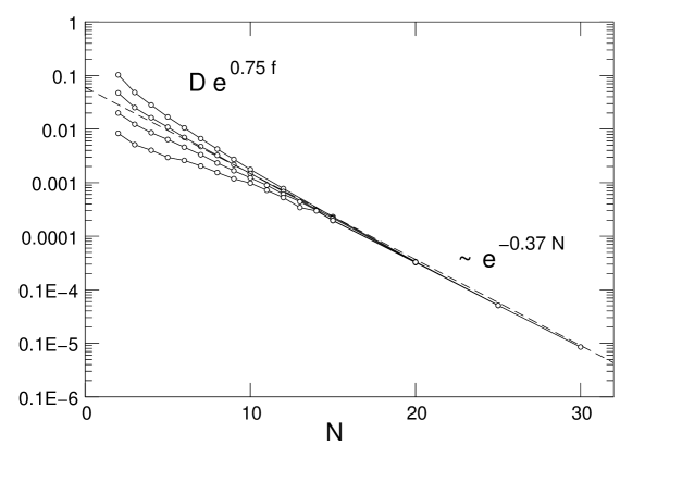
FIG. 2.: Semi-log plot of the Monte Carlo data of the scaled diffusion coefficients $D{\rm e}^{0.75f}$ for $3\leq f\leq 6$ and $2\leq N\leq 30$. The broken line corresponds to $\sim{\rm e}^{-0.37N}$.

Assuming this exponential law we have analyzed the pre-exponential power law of (3). This is presented in Fig. 3. In agreement with previous simulations [6] and theoretical considerations [7] one observes for shorter chains an effective power law of $N^{-0.6}$, given by the broken line in Fig. 3. However, at $N>10$ there is a significant deviation from the initial behavior. The statistical error, as given in Table I, cannot account for this.

FIG. 3.: Log-log plot of the Monte Carlo data of the scaled diffusion coefficients $D{\rm e}^{0.75f+0.37N}$. The broken line corresponds to $\sim N^{-0.6}$. The numbers at each curve denote the number of arms $f$.

Therefore, we have reexamined the data assuming the exponential factor of Helfand and Pearson (2). The corresponding analysis is presented in Fig. 4. In this case the data indicate a pre-exponential power law of $N^{-2}$. Therefore, in the limit of large $N$ the data of the diffusion coefficient seem to obey the formula

$$D_{1}=N^{-2}\;{\rm e}^{-\alpha_{HP}N-0.75f+1.7}$$ (5)

(the subscript $``1^{\prime\prime}$ indicates the single star behavior trapped inside a fixed network, in contrast to the case of concentrated solutions of star polymers). It is interesting to note that the exponential term can be approximated by $\exp[-\alpha_{HP}N-0.75(f-2)]$.

FIG. 4.: Log-log plot of the Monte Carlo data of the scaled diffusion coefficients $D{\rm e}^{0.75f+0.29389N}$. The broken line corresponds to $\sim N^{-2}$. The numbers at each curve denote the number of arms $f$.

The normalized data $D/D_{1}$ are presented in Fig. 5.

FIG. 5.: Log-log plot of the Monte Carlo data of the scaled diffusion coefficients $D/D_{1}$, where $D_{1}$ is given by Eq. (5).

It is important to note that the $f$-dependence of $D_{1}$ appears as a pre-exponential factor. Previous suggestions [5, 15] assumed $D\sim\exp(-\alpha(f-2)N)$, based on the assumption that the diffusion of the branch point requires simultaneous retraction of all but two of the star arms. The latter approach cannot be reconciled with our data. However, there is a much better agreement between our data and recent estimates based on experiments [16] which gave $D\sim\exp(-0.41f)$. These two latter findings, Monte Carlo and experiments, strongly support earlier considerations by Rubinstein [17] who predicted a much weaker dependence on $f$ as compared to the prediction $\exp(-\alpha fN)$. Therefore the experimental work [16] and our analysis strongly support the view that in order to move the center of the star, the $f-2$ arms need not be retracted simultaneously. Our data cannot be used to distinguish clearly between Rubinstein’s [17] and our formula $\exp(-0.75f)$ as given in Eq.(5).

IV Summary and Conclusions

We have reported on Monte Carlo results of diffusion coefficients of lattice star polymers trapped inside a fixed network. We found that our data are in agreement with the Helfand-Pearson exponential factor $\alpha=0.29$. However, the pre-exponential power law exponent $\beta=2$ is different from existing theories and coincides with the exponent for linear chains. In contrast to existing theoretical predictions, we found that the number of arms $f$ leads to a pre-exponential factor of the form $\exp(-0.75f)$.

We have not undertaken to estimate the finite size corrections to the asymptotic formula (3) using our Monte Carlo data. This would be probably quite useful comparing our results with more refined theories proposed recently [19].

Acknowledgements We are grateful to an anonymous referee for pointing out references [16] and [17].

REFERENCES

- [1] Kraus, G.; Gruver, J. T. J. Polym. Sci. 1965, A3, 105.
- [2] Fetters, L. J.; Kiss, A. D.; Pearson, D. S.; Quack, G.; Vitus, F. J. Macromolecules 1993, 26, 647.
- [3] de Gennes, P. G. J. Phys. (France) 1975, 36, 1199.
- [4] Doi, M.; Kuzuu, N. Y. J. Polym. Sci. Lett. 1980, 18, 775.
- [5] Graessley, W. W. Adv. Polym. Sci. 1982, 47, 67.
- [6] Needs, R. J.; Edwards, S. F. Macromolecules 1983, 16, 1492.
- [7] Pearson, D. S.; Helfand, E. Macromolecules 1984, 17, 888.
- [8] Helfand, E.; Pearson, D. S. J. Chem Phys. 1983, 79, 2054.
- [9] Evans, K. E. J. Chem. Soc., Faraday Trans. 2 1981, 77, 2385.
- [10] Rubinstein, M. Phys. Rev. Lett. 1987 59, 1946.
- [11] Barkema, G. T.; Marko, J. F.; Widom, B. Phys. Rev. E 1994, 49, 5303.
- [12] Barkema, G. T.; Newman, M. E. J. Physica A 1997, 244, 25.
- [13] Newman, M. E. J.; Barkema, G. T. Phys. Rev. E 1997, 56, 3468.
- [14] Barkema, G. T.; Krenzlin, H. M. J. Chem. Phys. 1998, 109, 6486.
- [15] Doi, M.; Edwards, S. F. The Theory of Polymer Dynamics, Clarendon Press, Oxford, 1986, p. 215.
- [16] Shull, K. R.; Kramer, E. J.; Fetters, L. J. Nature 1990, 345, 790.
- [17] Rubinstein, M. Phys. Rev. Lett. 1986 57, 3023.
- [18] Klein, J. Macromolecules 1986, 19, 105.
- [19] Milner, S. T.; McLeish, T. C. Macromolecules 1997, 30, 2159.