[

Spin Bose Glass Phase in Bilayer Quantum Hall Systems at $\nu=2$

Abstract

We develop an effective spin theory to describe magnetic properties of the $\nu=2$ Quantum Hall bilayer systems. In the absence of disorder this theory gives quantitative agreement with the results of microscopic Hartree-Fock calculations, and for finite disorder it predicts the existence of a novel spin Bose glass phase. The Bose glass is characterized by the presence of domains of canted antiferromagnetic phase with zero average antiferromagnetic order and short range mean antiferromagnetic correlations. It has infinite antiferromagnetic transverse susceptibility, finite longitudinal spin susceptibility and specific heat linear in temperature. Transition from the canted antiferromagnet phase to the spin Bose glass phase is characterized by a universal value of the longitudinal spin conductance.

]

Recently a canted antiferromagnetic phase has been predicted in bilayer quantum Hall (QH) systems at a total filling factor $\nu=2$ on the basis of microscopic Hartree-Fock calculations and a long wavelength quantum $O(3)$ nonlinear sigma model [1]. In this letter we construct an alternative effective spin theory that can describe the richness of the phase diagram of a bilayer $\nu=2$ quantum Hall system. Our effective spin theory treats the interlayer tunneling nonperturbatively, in contrast to the O(3) nonlinear sigma model which includes tunneling perturbatively through an antiferromagnetic exchange. It gives excellent agreement with the results of microscopic Hartree-Fock calculations in [1] and extends the earlier effective field theory by allowing to study quantitatively the effect of a finite gate-voltage between the layers and calculate intersubband excitation energies. Our theory can easily incorporate the effects of disorder and we predict that for any non-zero disorder there is a new $\nu=2$ spin Bose glass quantum Hall phase which may be visualized as domains of canted antiferromagnetic phase surrounded by domains of fully polarized ferromagnetic or spin singlet phases. In this system the Bose glass phase we predict is quite novel, and we elaborate in this Letter on the origin and the properties of this new QH glass phase. Related disorder induced spin phase has been discussed in a different setting in reference [2].

In the absence of interlayer interaction each layer of the $\nu=2$ bilayer system would be in a fully spin polarized ferromagnetic $\nu=1$ incompressible QH state with spins in both layers pointing in the direction of the applied magnetic field (FPF state). Tunneling between the layers favors the formation of spin singlet states from the pairs of electrons in the opposite layers and energetically stabilizes the spin singlet (SS) state. In [1] it was observed that the competition between the two tendencies may lead to a third intermediate phase: canted antiferromagnetic state, where spins in the two layers have the same component along the applied field but opposite components in the perpendicular 2D plane (CAF state).

We now introduce a simple lattice model which we use to describe the physics of the bilayer $\nu=2$ QH system. We consider a bilayer lattice model shown in figure 1.

FIG. 1.: Effective bilayer lattice model for $\nu=2$ double layer QH system

Sites in each layer may be thought of as labeling different intra-Landau-level states. Electrons may tunnel from one layer to another conserving the in-plane site index (i.e. between the states with the same intra-Landau-level index). There is a ferromagnetic interaction between nearest-neighbor sites within individual layers and a Zeeman interaction with the applied magnetic field. We also account for the charging energy, i.e. the energy cost of creating charge imbalance between the layers through the term ${\cal H}_{c}$ below. The Hamiltonian of the system may be written as

$${\cal H} = {\cal H}_{T}+{\cal H}_{c}+{\cal H}_{Z}+{\cal H}_{F}$$ (1)

$${\cal H}_{T} = -\frac{1}{2}\Delta_{SAS}\sum_{i}(c_{Ti\sigma}^{\dagger}c_{Bi\sigma}+c_{Bi\sigma}^{\dagger}c_{Ti\sigma})$$ (2)

$${\cal H}_{c} = \frac{1}{2}\epsilon_{c}\sum_{i}\left((n_{Ti}-1)^{2}+(n_{Bi}-1)^{2}\right)$$ (3)

$${\cal H}_{Z} = -H_{z}\sum_{i}(S^{z}_{Ti}+S^{z}_{Bi})$$ (4)

$${\cal H}_{F} = -J\sum_{\langle ij\rangle}({\bf S}_{Ti}{\bf S}_{Tj}+{\bf S}_{Bi}{\bf S}_{Bj})$$ (5)

where $T$ or $B$ is the isospin index that labels electrons in the top and bottom layers respectively, $i$ is the in-plane site ( intra-Landau-level ) index, and $\sigma$ is the spin index. ${S}^{a}_{Ti}=c_{Ti\alpha}^{\dagger}{\bf\sigma^{a}_{\alpha\beta}}c_{Ti\beta}$ and $n_{Ti}=\sum_{\sigma}c_{Ti\sigma}^{\dagger}c_{Ti\sigma}$ are spin and charge operators for layer $T$, with analogous definitions for layer $B$. Parameters $J$ and $\epsilon_{c}$ of this model may be easily estimated as $\rho_{S}^{0}=e^{2}/(16\sqrt{2\pi}\epsilon l)$ , where $l=\sqrt{\hbar c/eB}$ is magnetic length and $\epsilon_{c}=\frac{e^{2}}{\epsilon l}\sqrt{\frac{\pi}{2}}(1-e^{-d^{2}/l^{2}}Erf[d/(l\sqrt{2})])$, where $d$ is the distance between the layers and $Erf$ is the error function [3].

Let us consider an individual rung, i.e. two sites with the same in-plane site index on the opposite layers. Each rung must be populated by two electrons, therefore we have six possible states for each rung. The six available states are conveniently classified into three states that are spin triplets

$$\begin{array}[]{ll}|t_{+}\rangle=t_{+}^{\dagger}|0\rangle&=c_{T\uparrow}^{\dagger}c_{B\uparrow}^{\dagger}|0\rangle\\ |t_{0}\rangle=t_{0}^{\dagger}|0\rangle&=\frac{1}{\sqrt{2}}\left(c_{T\uparrow}^{\dagger}c_{B\downarrow}^{\dagger}+c_{T\downarrow}^{\dagger}c_{B\uparrow}^{\dagger}\right)|0\rangle\\ |t_{-}\rangle=t_{-}^{\dagger}|0\rangle&=c_{T\downarrow}^{\dagger}c_{B\downarrow}^{\dagger}|0\rangle\end{array}$$ (9)

and three states that are spin singlets

$$\begin{array}[]{ll}|\tau_{+}\rangle=\tau_{+}^{\dagger}|0\rangle&=c_{T\uparrow}^{\dagger}c_{T\downarrow}^{\dagger}|0\rangle\\ |\tau_{0}\rangle=\tau_{0}^{\dagger}|0\rangle&=\frac{1}{\sqrt{2}}\left(c_{T\uparrow}^{\dagger}c_{B\downarrow}^{\dagger}-c_{T\downarrow}^{\dagger}c_{B\uparrow}^{\dagger}\right)|0\rangle\\ |\tau_{-}\rangle=\tau_{-}^{\dagger}|0\rangle&=c_{B\uparrow}^{\dagger}c_{B\downarrow}^{\dagger}|0\rangle\end{array}$$ (13)

Operators $t$ and $\tau$ satisfy bosonic commutation relations [4] and constraint $\tau_{\alpha}^{\dagger}\tau_{\alpha}+t_{\alpha}^{\dagger}t_{\alpha}=1$ projects into the physical Hilbert space.

In Hamiltonian (5) all the terms except ${\cal H}_{F}$ act within a single rung. It is therefore natural as a first step to diagonalize ${\cal H}^{\prime}={\cal H}_{T}+{\cal H}_{c}+{\cal H}_{Z}$ on one rung. The latter task is simplified by the observation that ${\cal H}_{T}$ and ${\cal H}_{c}$ act in the subspace of $\tau$ states, whereas ${\cal H}_{Z}$ operates in the $t$ subspace. A simple calculation gives for the lowest energy eigenstates of ${\cal H}^{\prime}$:

• state $|t_{+}\rangle$ with energy $E_{t}=-H_{z}$

• state $|v_{+}\rangle=\frac{(\sin\theta-\cos\theta)}{2}(|\tau_{+}\rangle+|\tau_{-}\rangle)-\frac{(\sin\theta+\cos\theta)}{\sqrt{2}}|\tau_{0}\rangle$
  with energy $E_{v}=\frac{\epsilon_{c}}{2}-\sqrt{\Delta_{SAS}^{2}+\epsilon_{c}^{2}/4}$. Here $\tan\theta=\epsilon_{c}/(2\Delta_{SAS}+2\sqrt{\Delta_{SAS}^{2}+\epsilon_{c}^{2}/4})$

State $|v_{+}\rangle$ is a spin-singlet state whose energy is lowered by interlayer tunneling and $|t_{+}\rangle$ is a spin triplet state favored by Zeeman interaction. Competition between the two states is a competition between the SS state and the FPF state. In the absence of the in-plane ferromagnetic interaction we would have level crossing at $E_{v}=E_{t}$ with a first order phase transition between SS and FPF phases. However as we show below ${\cal H}_{F}$ acts as an interaction that connects the two states and gives rise to an intermediate state that is a superposition of the $|v_{+}\rangle$ and $|t_{+}\rangle$ states and corresponds to the CAF phase.

We rewrite Hamiltonian (5) keeping only the lowest energy states $|v_{i+}\rangle$ and $|t_{i+}\rangle$:

$$\tilde{{\cal H}}=E_{t}\sum_{i}t_{i+}^{\dagger}t_{i+}+E_{v}\sum_{i}v_{i+}^{\dagger}v_{i+}$$ (14)

$$- \frac{J}{4}(\cos\theta+\sin\theta)^{2}\sum_{\langle ij\rangle}\left(t_{i+}^{\dagger}v_{i+}v_{j+}^{\dagger}t_{j+}+t_{j+}^{\dagger}v_{j+}v_{i+}^{\dagger}t_{i+}\right)$$ (15)

$$- \frac{J}{2}\sum_{\langle ij\rangle}t_{i+}^{\dagger}t_{i+}t_{j+}^{\dagger}t_{j+}$$ (16)

and the hard core constraint is implied

$$v_{i+}^{\dagger}v_{i+}+t_{i+}^{\dagger}t_{i+}=1$$ (17)

The mean field analysis of Hamiltonian (16) may be done by considering states with simultaneously condensed $v$ and $t$ bosons. They correspond to the variational wavefunctions of the form $|\Psi\rangle=exp\{\alpha\sum_{i}v_{i+}^{\dagger}+\beta\sum_{i}t_{i+}^{\dagger}\}|0\rangle$ [4]. The energy of state $|\Psi\rangle$ is given by

$$E_{0}=E_{v}|\alpha|^{2}+E_{t}|\beta|^{2}-J(\cos\theta+\sin\theta)^{2}|\alpha|^{2}|\beta|^{2}-J|\beta|^{4}$$ (18)

and state $|\Psi\rangle$ obeys constraint (17) on the average provided that

$$|\alpha|^{2}+|\beta|^{2}=1$$ (19)

Values of $\alpha$ and $\beta$ that minimize (18) under the condition (19) are given by

$$\begin{array}[]{lll}|\alpha|=1&|\beta|=0&if~{}t_{min}<0\\ |\alpha|=t_{min}&|\beta|=\sqrt{1-t_{min}^{2}}&if~{}0<t_{min}<1\\ |\alpha|=0&|\beta|=1&if~{}t_{min}>1\end{array}$$ (23)

where

$$t_{min}=\frac{J(\cos\theta+\sin\theta)^{2}-E_{t}+E_{v}}{2[J(\cos\theta+\sin\theta)^{2}-J]}$$ (24)

The first and the last cases obviously correspond to the FPF and SS phases respectively [5]. But there is also a nontrivial new phase that appears in our analysis when both $|\alpha|$ and $|\beta|$ are finite. It is easy to verify that this state corresponds precisely to the canted antiferromagnetic phase discussed in [1] with direction of the Neel ordering given by the phase between the $t_{+}$ and $v_{+}$ condensates $tan^{-1}N_{y}/N_{x}=Arg(\alpha^{*}\beta)$ ( Neel order parameter is defined as ${\bf N}=\sum_{i}{\bf S}_{Ti}-\sum_{i}{\bf S}_{Bi}$ ). On figure 2 we show the phase diagram obtained from equation (23). We can also use our bosonic model to calculate the phase diagram in the presence of an interlayer charge imbalance and these results will be reported elsewhere [3].

The lowest energy interband transition in the SS phase will correspond to destroying a $v_{+}$ and creating a $t_{+}$ boson. The energy for such transition is $\omega_{-}=-J(cos\theta+sin\theta)^{2}+E_{t}-E_{v}$ and vanishes at the SS/CAF transition as may be seen from equations (23) and (24). Analogously in the FPF state the lowest energy interband transition will correspond to destroying $t_{+}$ and creating a $v_{+}$ boson [3].

FIG. 2.: Phase diagram for disorder-free system. All energies are in units of $J$, $\epsilon_{c}=5.0J$.

Let us now give a simple physical picture that will illustrate formal calculations presented above. We consider an SS state which has singlet $v_{+}$-bosons on all rungs and imagine creating $t_{+}$-triplet on one of the rungs. Creating a localized triplet requires energy $E_{t}-E_{v}$ and this energy is unaffected by the ferromagnetic interaction since parallel and anti-parallel contributions cancel for triplet interacting with neighboring singlets. However ${\cal H}_{F}$ also gives rise to a process in which one of the spins of the triplet pair and one spin from the neighboring singlet pair are flipped simultaneously. This process is shown on figure 3 and may be interpreted as hopping of the triplet boson to the nearest-neighbor site. Therefore creating a propagating triplet boson at wavevector $k$ will give it an additional kinetic energy $\tilde{J}(cosk_{x}+cosk_{y})$ due to ${\cal H}_{F}$. This allows us to have a situation when $E_{t}-E_{v}>0$ but $E_{t}-E_{v}-2\tilde{J}<0$, i.e. when it is energetically unfovarable to create localized triplets but it is already favorable to create them at $k=0$, i.e. to have a condensate of $t_{+}$ bosons. This effect is the origin of the CAF state and allows us to understand this phase as a coherent superposition of condensed $t_{+}$ and $v_{+}$ bosons.

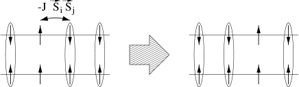
FIG. 3.: Triplet “hopping” process due to ferromagnetic in-pane interaction

In a real system there is always disorder. It may be due to fluctuations in the distance between the wells or the presence of impurities. Such disorder can be easily included in our effective bosonic theory, but would be difficult if not impossible, to include in the Hartree-Fock theory of references [1]. For our effective spin model the major effects of disorder will be randomness in the value of tunneling $\Delta_{SAS}$ and the appearance of a random local gate voltage, in both cases leading to random local fluctuations in the energy of the $v_{+}$ boson. Then if we are close to the CAF-SS transition we may have a situation induced by disorder where $E_{t}-E^{max}_{v}-2\tilde{J}<0$ and $E_{t}-E^{min}_{v}-2\tilde{J}>0$. So for some regions creating non-local $t_{+}$ triplets will lower the energy of the system and for some regions it will lead to an energy increase. In this case the system breaks into domains, with each domain being locally a CAF phase or a SS phase (region III on figure 4). Each CAF domain may be thought of as being in a quantum disordered state with an undefined direction of the Neel order but finite z-magnetization [2]. Close to the CAF-FPF transition line in the disorder-free system we may have a disorder induced situation where we have CAF domains in the background of domains of the FPF phase (region I on figure 4). Finally we can also have the phase where we have domains of all three kinds ( region II on figure 4 ). In figure 4 we show the resulting phase diagram for the same values of parameters as in figure 2 but assuming that $\Delta_{SAS}$ may randomly vary by 10% around its average value. Such a variation in $\Delta_{SAS}$ is physically quite reasonable even in high quality 2D systems since $\Delta_{SAS}$ depends exponentially on layer thickness. There are no phase transitions between regions I, II and III on the phase diagram in figure 4 but only smooth crossovers. The true quantum phase transitions occur between FPF and I, SS and III and between CAF and one of the I, II or III regions.

FIG. 4.: Phase diagram for a disordered system. All energies are in units of $J$, $\epsilon_{c}=5~{}J$. Variation in $\Delta_{SAS}$ was assumed to be 10 %. Region I corresponds to domains of CAF and FPF phases, Region III to domains of SS and CAF and region II to domain of all three kinds. There are no phase transitions among regions I, II, III, they all correspond to the spin Bose glass phase.

The nature of these phase transitions is also easy to understand. The SS phase is an insulating phase of zero density of $t_{+}$ bosons, FPF state is an insulating phase with density $n=1$[5] and CAF is a superfluid phase. Randomness that we consider acts as a randomness in the chemical potential of these $t_{+}$ bosons, so our problem is equivalent to the problem of bosons in a random potential, the so-called dirty boson problem, considered in references [6, 7]. We immediately recognize I, II and III as a single Bose glass (SBG) phase of the singlet and triplet bosons. This observation allows us to draw several important conclusions about the properties of this SBG phase. In the SS state the $\langle S^{z}(-\omega)S^{z}(\omega)\rangle$ correlation function is zero and in the CAF phase it has a $\delta$-function peak at zero frequency due to the Goldstone mode of the spontaneous breaking of the $U(1)$ symmetry of spin rotations around the $z$-axis. In the SBG phase this correlation function will be finite at small frequencies, which implies finite longitudinal spin susceptibility and is the analog of finite compressibility of the usual charge Bose glass. Our new SBG phase does not have antiferromagnetic long range order, i.e. $\langle N_{x(y})\rangle=0$. All the $t_{+}$ and $v_{+}$ bosons are localized in this phase, therefore it will have only short range mean antiferromagnetic correlations. But analogous to the infinite superfluid susceptibility of charge Bose glass our SBG phase will have an infinite transverse antiferromagnetic susceptibility. Another important feature of the Bose glass phase is a finite density of low energy excitations [6, 7]. This implies that our SBG phase will have a specific heat linear in temperature which provides another way to experimentally distinguishing it from the CAF phase whose specific heat goes as $T^{2}$ or FPF and SS phases that have exponentially small specific heat at low temperatures. The existence of the SBG phase separating SS, FPF and CAF phases also has important consequences in that it changes the critical exponents for the corresponding phase transitions from the one obtained in [1] for the disorder-free system. The new critical exponents will be those of the superconductor-insulator transition in dirty boson system studied in [6, 7]. We would also like to point out that the SBG system that we suggested may be a better experimental realization of a 2d superconductor-insulator transition in a boson system than conventionally used 2d superconducting films [8] in that it is free of long range forces and allows one to vary the density of bosons by varying $H_{z}$. In addition our predicted QH Bose glass phase transition does not have the complication arising from parallel fermionic excitations which may play a role in the superconducting films [9]. We therefore expect, based on the arguments given in [6, 7], that transition from the CAF phase to the SBG phase will be characterized by a truly universal longitudinal spin conductance, which in principle can be measured by measuring the spin susceptibility and the spin diffusion coefficient.

Before concluding we remark on the feasible experimental observability of our proposed QH Bose glass phase. First we remark that the basic $\nu=2$ QH phase transition and the associated softening of the relevant spin density excitations has been verified experimentally [10] via inelastic light scattering spectroscopy. Since interlayer tunneling fluctuations are invariably present in real systems, it is in fact quite possible that the experiments in [10] have already observed a transition to the Bose glass phase as in our figure 4. Some evidence supporting this possibility comes from the fact that softening of the spin density excitations observed in [10] did not lead to the appearance of a sharp dispersing Goldstone mode expected in the CAF phase but only to some broad zero energy spectral weight consistent with the Bose glass phase. Future experiments in samples with deliberately controlled disorder should be carried out to conclusively verify our prediction of a QH disordered Bose glass phase.

In conclusion we predict a new 2D Bose glass phase in a $\nu=2$ QH bilayer system by introducing an effective spin theory. This phase has the usual properties of a Bose glass phase [6, 7] including a universal spin conductance at the transition. While we have specifically considered the $\nu=2$ integer QH situation, our arguments should go through for all $\nu=2/$(odd integer) fractional QH states also, following the reasoning of [1], and for the fractional filling there should be an exotic fractional quantum 2D Bose glass in bilayer systems[11].

This work is supported by the NSF at ITP and by the US-ONR (S.D.S.). We acknowledge useful discussions with M.P.A. Fisher, Y. Kim, A. MacDonald, R. Rajaraman, S. Sachdev, and T. Senthil.

REFERENCES

- [1] L. Zheng et. al. , Phys. Rev. Lett., 78:2453 (1997); S. Das Sarma et. al. , Phys. Rev. Lett., 79:917 (1997); S. Das Sarma et. al. , Phys. Rev. B 58:4672 (1998)
- [2] T. Senthil and S. Sachdev, Annals of Physics 251:76 (1996)
- [3] E. Demler and S. Das Sarma, unpublished
- [4] S. Sachdev and R. Bhatt, Phys. Rev. B 41:9323 (1990);
- [5] In our variational wavefunctions the FPF phase is described as a superfluid state of bosons with average density rather than an insulating state with exactly one -boson per site. This is a result of our mean-field treatment of the hard core constraint (19). Analogously the SS state in our mean-field calculations appears as a superfluid of bosons with one boson per site on the average and not as an insulator with exactly one boson per site.
- [6] M.P.A. Fisher et. al. , Phys. Rev. B 40:546 (1989); M.P.A. Fisher et. al. , Phys. Rev. Lett., 64:587 (1990)
- [7] M. Cha et. al. , Phys. Rev. B 44:6883 (1991); M. Wallin et. al. , Phys. Rev. B 49:12 115 (1994)
- [8] A. Hebard and M. Paalanen, Phys. Rev. Lett. 65:587 (1990); Y. Liu et. al. , Phys. Rev. B 47:5931 (1993); A. Yazdani and A. Kapitulnik, Phys. Rev. Lett. 74:3037 (1995)
- [9] K. Hagenblast et. al. , Phys. Rev. Lett. 78:1779 (1997);
- [10] V. Pellegrini et. al. , Phys. Rev. Lett. 79:310 (1997); V. Pellegrini et. al. , Science 281:799 (1998)
- [11] Another plausible effect of disorder, which we do not discuss in this paper, is the appearance of unmatched spins leading to the possibility of a random-singlet phase. This effect is not important at but may become relevant for the (odd integer) fractional QH states.