[

Time scale separation and heterogeneous off-equilibrium dynamics in spin models over random graphs

Abstract

We study analytically and numerically the statics and the off-equilibrium dynamics of spin models over finitely connected random graphs. We identify a threshold value for the connectivity beyond which the loop structure of the graph becomes thermodynamically relevant. Glauber dynamics simulations show that this loop structure is responsible for the onset of dynamical features of a local character (dynamical heterogeneities and spontaneous time scale separation), consistently with previous (experimental and numerical) studies of glasses and spin glasses in their approach to the low temperature phase.

]

Among the characteristic features of the equilibrium and off–equilibrium behavior of complex physical systems such as glasses or granular materials, two basic ones are the heterogeneities occurring in the spatial distribution of particles and the time scale separation in the relaxation processes of the different degrees of freedom [3, 4, 5, 6]. The issue of building a clear connection between such local structures and the global relaxation process is currently an open basic topic. In this context, simple spin models have played a crucial role, both for the analytical studies which have provided a possible mean–field theory of the glass transition [7] and for numerical simulations. In particular, the study of mean field spin–glasses with infinite connectivity has allowed to understand some features of both the statics [8] and dynamics of the glassy phase [9]. However, intrinsic to the above models is the topology of the connections which cannot account for any local structure, each site being connected with all others.

In this Letter, we will discuss the relationship between the topology of interactions, in the spirit of random networks [10, 11], and the onset of heterogeneous glassy dynamics in models which allow some analytical understanding, namely interacting spin models defined over random graphs with finite connectivity. We will provide analytical and numerical results which clarify some basic differences between infinitely connected and finitely connected mean field spin models and, more interestingly, identify a simple link between the loop structure of the random lattice, the nature of the couplings and the glassy heterogeneous dynamics. As we shall discuss, in finitely connected mean field models the non–trivial underlying topological structure of the links is responsible for the appearance of non–equilibrium phenomena of local nature (both in space and time) and the numerical results turn out to be in remarkable agreement with those of finite dimensional systems. Interestingly enough, our results appear also to be related with the so called “small-world” dynamical patterns discussed in ref. [12], of relevance in contexts different from physics, e.g. biological oscillators, neural networks, spatial games and genetic control networks: all these problems are indeed defined over random graphs where the typical separation between two vertices in the graph is much lower than in regular graphs, allowing for a quick spread out of dynamical correlations over the network (see [12] and references therein for a more detailed discussion).

Given a graph ${\cal G}=(V,E)$, where $V$ is the set of $N$ vertices and $E$ is the set of bonds joining $K=2$ (graphs) or $K>2$ (hyper-graphs) vertices, the spin Hamiltonians take the form

$$H=\sum_{i_{1}<...<i_{K}\in V}J_{i_{1},...,i_{K}}\,S_{i_{1}}\cdots S_{i_{K}}\;\;,$$ (1)

where the indices $i_{1},...,i_{K}$ run over the set $V$ of $N$ vertices, each vertex $i$ bearing an Ising spin $S_{i}$, and the couplings $J_{i_{1},...,i_{K}}$ associated to the random bonds assume values of order one (to be compared with $O(1/\sqrt{N})$ as in usual infinitely connected models). We consider graphs with finite connectivity, in which the notion of distance is simply the minimal number of bonds on a path connecting two sites, also referred to as chemical distance.

In the study of random (hyper)graphs the control parameter is the average density of bonds, $\gamma$ (or the average connectivity $C=K!\gamma$). For densities small enough, the graph consists of many small connected clusters of size $O(\ln N)$. If $\gamma$ increases up to the percolation value $\gamma_{c}$, there appears a spanning cluster containing a finite fraction of the $N$ sites in the limit of large $N$. However, such a spanning cluster can a priori have a tree-like structure, for which the randomness of the couplings $J_{i_{1},...,i_{K}}=\pm 1$ can be eliminated by a gauge transformation on the spins (just like in the one-dimensional random bonds Ising model). This leads to the definition of a second threshold value for the density $\gamma$, defined as that critical density $\gamma_{0}$ at and beyond which frustration in the system cannot be removed by such a gauge transformation, and therefore gives a macroscopic contribution to the thermodynamics, raising both internal energy and entropy in the system. Geometrically this threshold corresponds to the appearance of an extensive number of loops in the spanning cluster and it has been named percolation of order (PO) transition in ref. [13]. While, for random $K=2$ graphs, the two transitions are known to coincide [13], here we shall study the $K=3$ hypergraph structure. While the notion of loops in hypergraphs is rather counter intuitive, the idea of frustration retains its simple physical interpretation. The study of the onset of frustration in the ground state phase diagram of the associated random $K=3$ spin glass model, will allow us to show that the percolation transition $\gamma_{c}$ and the PO transition $\gamma_{0}$ are well separated. Interestingly enough, by resorting to extensive Glauber dynamics simulations, we shall also show that such a change in the graph structure is responsible for the onset of heterogeneous glassy dynamics.

As discussed in refs. [14, 15], the most striking geometrical feature characterizing the ground state phase diagram of frustrated spin models over finite connectivity random graphs above the PO transition, is that, in spite of a finite entropy per site, there exists a finite fraction of spins which is totally constrained, a “backbone” that does not change from state to state (strongly reminiscent of rigidity percolation [16]). The remaining fraction of spins is weakly constrained and accounts for the overall exponential degeneracy of the ground state.

Here we are interested in the dynamical, off–equilibrium, consequences of such a structure consisting, as we shall see, in a spontaneous separation of weakly constrained spins (i.e. dynamically fast) and strongly constrained ones, leading to time scale separation and heterogeneous dynamics at sufficiently low temperatures. Such a behavior, by definition typical of glassy systems [4], turns out, for $K\geq 3$, to be independent on the frustration of the couplings in that the underlying loop structure together with the K–body interaction lead to an annealed self–induced “geometrical” frustration.

$K=3$ hypergraphs are constructed as follows: given $N$ sites, we choose at random $\gamma N$ triplets $(i,j,k)$ for which the couplings $J_{ijk}$ will be non zero. For $\gamma$ greater than the percolation value $\gamma_{c}=1/3$ ($\gamma_{c}=\frac{2}{K(K-1)}$ for K–spin couplings), we obtain, as previously explained, a spanning cluster of connected sites, containing a finite fraction of the $N$ spins in the large $N$ limit, and many other smaller (order $\log N$) disconnected clusters [18].

The PO transition is simply identified by comparing the ground state energy of the random $J_{ijk}=\pm 1$ system with that of the ferromagnetic system defined over the same hypergraphs. The value of $\gamma$ beyond which the two energies start to deviate identifies $\gamma_{0}$. Such a calculation allows to identify a wide gauge region, $\gamma_{c}<\gamma<\gamma_{0}$, where the relevant structure of the spanning cluster is tree–like.

Within the so called Replica Symmetric (RS) functional framework of diluted spin glasses [17], we find a first order PO transition at $\gamma_{0}^{RS}\simeq 0.9$, characterized by a finite backbone and finite entropy at the threshold. Such a result was derived by adopting the full RS iterative scheme discussed in ref. [14] in the resolution of the self–consistency equation for the $T=0$ probability distribution of the effective local fields $P(h)=2R(h/2)$ (in the notation of ref. [14]), which is given by $R(y)=\int_{-\infty}^{\infty}\frac{dx}{2\pi}\cos(xy)\exp\left\{-9\gamma(1-\phi[R;x])\right\}$ where $\phi[R;x]=\int_{-\infty}^{\infty}dz_{1}dz_{2}R(z_{1})R(z_{2})\cos[x\,{\rm min}(1,|z_{1}|,|z_{2}|)]$. Looking for solutions of the form $R(y)=\sum_{\ell=-\infty}^{\infty}r_{\ell}\;\delta\left(y-\frac{\ell}{p}\right)$, where $1/p$ is the resolution of the field which eventually goes to zero, one obtains a set of $p+1$ coupled equations in the independent variables $\{r_{\ell}\}$ ($\ell=0,1,...,p$). Once this set has been solved, the ground state energy can be easily derived and compared with that of the corresponding ferromagnetic model, which, as expected, is simply proportional to the average connectivity and corresponds to the trivial $r_{\ell}=0$ ($\ell\neq 0$) and $r_{0}=1$ RS solution. While the exact identification of the threshold value $\gamma_{0}$ would require a full Replica Symmetry Breaking solution, indeed an open problem, the qualitative features of the phase transition are correctly identified already at the RS level [20]. In order to check this fact, we have done exhaustive enumeration of finite systems with sizes $N=18,20,...28$ (averaged over $18000,15000,...3000$ samples respectively). The extrapolated value for the threshold is $\gamma_{0}\simeq 0.8-0.9$ (with a value of the backbone at the transition of $\sim 0.2$), slightly below $\gamma_{0}^{RS}$ ($\sim.9$ for $p=15$) as expected. However, both the nature of the phase transition and the dependence of the ground state energy on $\gamma$ for large connectivity are consistent with the RS solution.

For brevity, here we do not report explicitly the details of the above analysis (a similar calculation is thoroughly described in ref. [14]), but rather focus on the dynamical consequences of the topological structure arising from the ground state analysis. Results from extended Glauber dynamics simulations performed over various graphs and Hamiltonians, indeed, confirm the appearance of the expected time scale separation and heterogeneous structure of the dynamics in the low temperature phase, where the systems are out of equilibrium at all times, and display aging dynamics. The topology of the connections rather than the form of the interactions appear to be the source of the robustness of the phenomenon. Such a feature is well known in models of glassy material[11].

The basic tool used to detect aging dynamics is the spin–spin correlation function, $C(t_{w}+t,t_{w})=\frac{1}{N}\sum_{i=1}^{N}\overline{\langle s_{i}(t_{w}+t)s_{i}(t_{w})\rangle}$, where $t_{w}$ is the so called waiting time and the average is taken over the spins, the thermal noise ($\langle.\rangle$) and the disorder (over-line): while, for equilibrium dynamics, $C(t_{w}+t,t_{w})$ depends only on $t$, aging is defined by the fact that $C(t_{w}+t,t_{w})$ depends also on $t_{w}$ for all times. To look for heterogeneities in a system, we have instead to study more local quantities, like local correlations $C_{i}(t_{w}+t,t_{w})=\langle s_{i}(t_{w}+t)s_{i}(t_{w})\rangle$ (averaged over the initial conditions), and the individual rates of flipping of the spins. For each spin, we can register during one Monte Carlo run the number of times it flips, and deduce the mean time $\tau_{i}$ between two spin-flips. Of course, the total running-time $\tau_{max}$ gives an upper cut-off. We can then look at the distribution of $\tau_{i}$, averaged over the samples, $\overline{P(\tau)}$ [19].

We have simulated graphs with either fixed connectivity ($4$ and $6$) or fluctuating connectivity (values of $C$ ranging from $3$ to $18$), and either ferromagnetic or random ($\pm 1$) couplings. To compute $\overline{P(\tau)}$, we used sizes from 500 to 5000 spins and a number of samples varying from 50 to 100. No relevant finite size effect was observed, consistently with the self–averaging character of $P(\tau)$. The dynamics has been implemented as a Glauber algorithm with random updating of the spins, with the runs mostly performed up to a time of $10^{6}$ Monte Carlo steps per spin. For consistency, we have also looked at times up to $10^{7}$ MC steps per spin for some samples.

At high temperature, we find of course a quite simple $\overline{P(\tau)}$, peaked at small values of $\tau$, i.e. high flipping rates, for all connectivities. However, as the temperature is lowered, we observe very different behaviors for different mean connectivities. Let us first concentrate on the case of fixed connectivity. For a random hyper-graph with connectivity $4$, $\overline{P(\tau)}$ is a smooth function peaked around a mean value (increasing as $\beta$ is lowered): the dynamics is homogeneous, and all the spins have more or less the same relaxation time (with fluctuations). For a fixed connectivity equal to $6$, on the contrary, we see that small values of $\tau$ still keep a finite weight, while a second part of the curve, corresponding to large times, emerges as $T$ decreases. This second part appears at temperatures for which aging dynamics sets in (i.e. at which $C(t_{w}+t,t_{w})$ becomes a function of both $t$ and $t_{w}$ for all times), thus signaling the onset of a glassy regime. The cusp in the curve, around $t^{*}\approx 10^{4}$ MC steps per spin, shows that a separation of time scales occurs. Such a cusp identifies “fast” and “slow” degrees of freedom, and persists for a large range of values of $\beta$: the fraction of fast spins, $\int_{0}^{t^{*}}\overline{P(\tau)}d\tau$, is a slowly decreasing function of $\beta$. For the case of connectivity $4$, $\int_{0}^{t^{*}}\overline{P(\tau)}d\tau$ shows instead a sharp transition when the mean value of the relaxation times crosses $t^{*}$. We show in figure (1) the two shapes of $\overline{P(\tau)}$, for connectivity $4$ and $6$, and the evolution of $\int_{0}^{t^{*}}\overline{P(\tau)}d\tau$ with $\beta$.

If we now consider random hyper-graphs with fluctuating connectivity, we observe a crossover between the two situations, as $\gamma$ (and therefore the mean connectivity $C$) is increased. Since the connectivity can vary from one site to another, the global $\overline{P(\tau)}$ can be decomposed in a sum of $\overline{P_{z}(\tau)}$, distributions of times $\tau_{i}$ restricted to the sites with connectivity $z$. Then, for $\gamma<\gamma_{0}$, the $\overline{P_{z}(\tau)}$ are smooth functions peaked around a mean value (evolving with $\beta$), while, as $\gamma$ grows, the $\overline{P_{z}(\tau)}$ becomes broader and broader, overlap with each other, and exhibits cusps [21]. The crossover occurs around $\gamma_{0}$ (note that mean connectivity $C=4$ corresponds to $\gamma<\gamma_{0}$, and mean connectivity $C=6$ to $\gamma>\gamma_{0}$), thus indicating that the loop structure is responsible for the appearance of complicated, inhomogeneous dynamics.

In order to understand the Glauber dynamics mechanisms on a microscopic level, we analyze in detail single samples of random hyper-graphs (with $\gamma>\gamma_{0}$). Rather than averaging over disorder, we compare single runs and average over initial conditions. Each single run (i.e. initial configuration) leads to a broad distribution of $\tau_{i}$. However, two cases may be distinguished. (I) if the connectivity can fluctuate from site to site, $\tau_{i}$ does not have a strong dependence on the initial conditions: if we call $\tau_{i}^{(1)}$ and $\tau_{i}^{(2)}$ the values of $\tau_{i}$ for two independent runs, we see in the inset of figure (2) that the histogram of the ratio $\tau_{i}^{(1)}/\tau_{i}^{(2)}$ is sharp and close to one. Thus, the broad distributions of $\tau_{i}$ lead to a broad distribution of $\langle\tau_{i}\rangle$, and the relaxations of the single site correlation functions $C_{i}(t,t^{\prime})$ depend strongly on the site $i$,(see Fig. 2). This shows that the position of the slow and fast degrees of freedom are encoded in the topology of the graph. (II) On the contrary, for random hyper-graphs with uniform connectivity, the histogram of figure (2) shows that the distribution of $\tau_{i}^{(1)}/\tau_{i}^{(2)}$ is broad (for a given site $i$, $\tau_{i}$ can vary a lot from one run to the other). It follows that $\langle\tau_{i}\rangle$ tends to a value independent of $i$ in the limit of many runs, and therefore $\langle s_{i}(t)s_{i}(t^{\prime})\rangle=\overline{\langle s_{i}(t)s_{i}(t^{\prime})\rangle}$. The slow or fast character of a spin depends on the initial conditions and is induced dynamically. Such a self induced frustration is probably more similar to what happens in real glasses.

Surprisingly enough, both for random and constant connectivity hyper-graphs, $\langle\tau_{i}\rangle$ does not depend on the nature of the couplings, either ferromagnetic or random. Once the loop structure of the graphs becomes irregular, frustration is totally induced by the dynamics through the initial conditions. For the sake of completeness, we have repeated the simulations on systems with Gaussian continuous couplings. All the discussed dynamical features are retained [22].

As a concluding remark, let us notice that, while the scope of this study was to show how mean field models could provide non–trivial local dynamical information, similar results are found in finite dimensional Edwards-Anderson spin glasses. In the latter case the topology of the lattice is fixed and the way of generating an effective non trivial topology is by randomly adding antiferromagnetic bonds to the ordinary Ising model [13]. For the Edwards-Anderson spin glasses with equally distributed ferro and antiferro bonds, we have also simulated aging dynamics in two and three dimensions [23], with the scope of pushing further the study of [5]. We indeed observe a similar shape for $\overline{P(\tau)}$. For ferromagnetic models on regular lattices instead, the well known coarsening relaxation process occurs: all spins are equivalent and no rich structure of $\overline{P(\tau)}$ or long-lasting spatial heterogeneities can be found. This is also true for spin models on quasi-periodic lattices, and on random graphs (i.e. with $K=2$ instead of $K=3$): the dynamics shows a similar $\overline{P(\tau)}$, with heterogeneities, only for random interactions (Viana-Bray model), and not for ferromagnetic ones.

We are most indebted to R. Monasson for valuable comments, and we thank S. Franz, S. Kirkpatrick, A. Maritan, D. Sherrington and A. Vespignani for discussions.

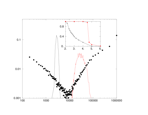
FIG. 1.: Typical examples of the distribution of times $\tau$ between two flips of a spin, $\overline{P(\tau)}$, for a hypergraph of $N=1000$ spins, with fixed connectivity; lines: connectivity $4$, $\beta=4$ and $\beta=5$; symbols: connectivity $6$, $\beta=3$; $t_{w}=10^{4}$ MC steps, $\tau_{max}=10^{6}$ MC steps. Inset: evolution of the fraction of fast spins, $\int_{0}^{t^{*}}\overline{P(\tau)}d\tau$ with $\beta$, for connectivity $4$ and $6$.

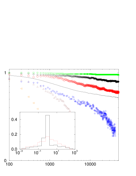
FIG. 2.: For one given random hypergraph, local autocorrelation function $C_{i}(t_{w}+t,t_{w})$ versus $t$ for various sites $i$ and a given $t_{w}$. For some sites $i$ $C_{i}$ decreases very fast, while for others it evolves very slowly. The line is the mean $C(t_{w}+t,t_{w})$. Here $N=1000$, $\gamma=1$, $\beta=3.5$, $t_{w}=10^{4}$ MC steps,and the mean is over $300$ runs. Inset: histograms of the ratios $\tau_{i}^{(1)}/\tau_{i}^{(2)}$ between two runs with different initial conditions for a random hypergraph with fixed connectivity (dotted line) and without (full line).

REFERENCES

- [1] Email: barrat@qcd.th.u-psud.fr; present address: L.P.T.H.E., Bâtiment 210, Université Paris-Sud, 91405 Orsay Cedex, France;
- [2] Email: zecchina@ictp.trieste.it.
- [3] See for example M. D. Ediger, C. A. Angell, and S. R. Nagel, J. Phys. Chem. 100, 13200 (1996); M. T. Cicerone and M. D. Ediger, J. Phys. Chem. 104, 7210 (1996).
- [4] Review on glasses in Science 267, 1924 (1995).
- [5] P. H. Poole, S. C. Glotzer, A. Coniglio, and N. Jan, Phys. Rev. Lett. 78, 3394 (1997).
- [6] W. Kob, C. Donati, S. J. Plimpton, P. H. Poole, and S. C. Glotzer, Phys. Rev. Lett. 79, 2827 (1997); C. Donati, J. F. Douglas, W. Kob, S. J. Plimpton, P. H. Poole, and S. C. Glotzer, Phys. Rev. Lett. 80, 2338 (1998).
- [7] T. R. Kirkpatrick and D. Thirumalai, Phys. Rev. B 36, 5388 (1987); G. Parisi, Il nuovo cimento 16, 939 (1994); M. Mézard and G. Parisi, J. Phys. A 29 6515 (1996); J.-P. Bouchaud, L. Cugliandolo, J. Kurchan and M. Mézard, Physica A 226, 243 (1996).
- [8] M. Mézard, G. Parisi, and M. A. Virasoro, Spin Glass Theory and Beyond, World Scientific, Singapore, 1987.
- [9] See for example J.-P. Bouchaud, L.F. Cugliandolo, J. Kurchan and M. Mézard, in World Scientific Spin Glasses and Random Fields, ed. A. P. Young; L. F. Cugliandolo and J. Kurchan, Phys. Rev. Lett. 71, 173 (1993).
- [10] J. C. Phillips, J. Non-Crystalline Solids 34, 153 (1979); 43, 37 (1981).
- [11] M. F. Thorpe, J. Non-Crystalline Solids 57, 355 (1983); J. C. Phillips, Phys. Today 35, 27 (1981).
- [12] D. Watts and S. Strogatz, Nature bf 393, 440 (1998).
- [13] A.J. Bray, S. Feng, Phys. Rev. B 36, 8456 (1987).
- [14] R. Monasson and R. Zecchina, Phys. Rev. Lett. 76, 3881 (1996) and Phys. Rev. E 56, 1357 (1997).
- [15] A. S. Gliozzi, R. Zecchina, unpublished.
- [16] D. J. Jacobs and M. F. Thorpe, Phys. Rev. Lett. 75, 4051 (1995); C. Moukarzel and P. M. Duxbury, Phys. Rev. Lett. 75, 4055 (1995).
- [17] L. Viana and A.J. Bray, J. Phys. C 18, 3037 (1985); I. Kanter and H. Sompolinsky, Phys. Rev. Lett 58, 164 (1987); H Orland, J. Physique Lett.46, L763 (1985); M. Mézard and G. Parisi, 46, L775 (1985); C. De Dominicis and P. Mottishaw, J. Phys. A 20, L1267 (1987); K. Y. M. Wong and D. Sherrington, J. Phys. A 21, L459 (1988); R. Monasson, J. Phys. A 31, 513 (1998).
- [18] In order to understand the effects of fluctuations in the site connectivity, in the simulations we have also considered random graphs with almost fixed connectivity. Such graphs can be generated by progressively adding bonds at random and saturating the connectivity condition for each site, stopping such a process when the connectivity condition is satisfied for at least of the sites.
- [19] Notice that this distribution is self-averaging: its shape is the same for every realization of the disorder, which means that the obtained features are valid for each.
- [20] In the similar case of the model which can be studied with very efficient recursive algorithms, the RS threshold provides an upper bound within of the numerical estimate [14].
- [21] The influence on the waiting time was also investigated. Of course depends on the two times, but the shape of is much less affected by : the effect of larger waiting times is just to saturate very slowly the fraction of frozen spins.
- [22] The only difference is that the distinction between fixed connectivity and fixed average connectivity disappears due to the additional fluctuations in the values of the couplings.
- [23] The critical temperature of the 2-dimensional Edwards-Anderson spin glass is 0, but, for low enough temperature, the system remains out of equilibrium for very long times, and, for a large enough system and not too long times, the overall behavior is the same as the one of a genuine low temperature phase.