Dynamics of defect formation

Abstract

A dynamic symmetry-breaking transition with noise and inertia is analyzed. Exact solution of the linearized equation that describes the critical region allows precise calculation (exponent and prefactor) of the number of defects produced as a function of the rate of increase of the critical parameter. The procedure is valid in both the overdamped and underdamped limits. In one space dimension, we perform quantitative comparison with numerical simulations of the nonlinear nonautonomous stochastic partial differential equation and report on signatures of underdamped dynamics.

When a system that undergoes a symmetry-breaking transition is swept through its critical point the initial symmetry is broken and domains are formed. Because of critical slowing down it is not possible to sweep adiabatically; the number of domains therefore depends on the rate of increase of the critical parameter. A new scenario for structure formation in the early universe and a proposal for its test in laboratory experiments resulted from the first understanding of the importance of this nonequilibrium effect [3]. Until recently, experimental [4] results tended to support the proposed scenario, but precise comparison was not possible because neither experiment nor theory was confident of more than exponents. The situation is now changing, with new experiments using quenches of liquid helium through the superfluid transition taking care to minimise vortex creation via flow processes [5]. In this Letter we report new theoretical results: precise expressions for the number of defects and quantitative agreement with numerical results.

The phenomenon of a dynamic transition has been studied in the zero-dimensional case (pitchfork bifurcation) in the context of lasers [6]–[12]. The time-dependence of the critical parameter produces a delay of the bifurcation given by $\sqrt{2\mu|\ln\epsilon|}$ where $\mu$ is the rate of increase of the parameter and $\epsilon$ the magnitude of additive fluctuations. Theoretical studies on spatially-extended systems revealed a characteristic distance between kinks. The spatial structure formed during the sweep through critical point from the symmetric to broken-symmetry regime is frozen in by the nonlinearity when, sufficiently far into the symmetry-broken regime, the system attains a metastable state [13, 14, 15, 16, 18]. Analytical progress is possible because the critical region is well-described by an equation which, although stochastic and non-autonomous, is linear. Here we consider the influence of inertia; we derive the scalings and signatures of the overdamped and underdamped limits.

The theory of dynamic transitions identifies three successive regimes in the evolution, as the critical parameter is increased. In the earliest regime, sufficiently far from the critical point, the evolution is quasi-adiabatic: the ensemble of field configurations is a small perturbation of that found for constant parameters [13, 18]. In the second region, close to the critical point, the system can no longer react quickly enough to the time-dependence of the critical parameter [3]. Our treatment based on the equation of motion, however, passes seamlessly between the first and second regions: in both, the field is everywhere small and precise calculation of the correlation function can be made from the linearized stochastic partial differential equation (SPDE) [13, 18]. We show that, for the purposes of calculating the number of kinks formed, the end of the second, nonequilibrium, region is the key. In the final region, the spatial structure consists of narrow kinks separating long regions where the field is close to one of the minima of the potential. The spatial structure is “frozen in” in the sense that the motion, merging and occasional nucleation of kink-antikink pairs happens on a slower timescale than the process that formed them. The separation of timescales is especially marked at high damping and low temperature [15].

We shall consider the specific example of the stochastic process in one space dimension satisfying the following nonautonomous SPDE [14, 16, 17]

$$\partial^{2}_{t}Y_{t}(x)-D\partial^{2}_{x}Y_{t}(x)+\gamma\partial_{t}Y_{t}(x)=$$ (1)

$$=g(t)Y_{t}(x)-Y_{t}(x)^{3}+\epsilon\,\eta(x,t).$$ (2)

The order parameter at time $t$ and position $x$, denoted by $Y_{t}(x)$, is a real-valued random variable. The last term in (2) is space-time noise, delta-function correlated in space and time: ${\big{<}\eta(x,t)\eta(x^{\prime},t^{\prime})\big{>}}=\delta(x-x^{\prime})\delta(t-t^{\prime})$. The fluctuation-dissipation relation is enforced by setting $\epsilon^{2}=2\gamma k_{B}\Theta$, where $\Theta$ is the temperature.

In our numerical simulations, the time-dependence of the critical parameter is: $g(t)=\mu t$, starting at $g=-\tau<0$. The initial conditions are

$$Y_{t_{0}}(x)=\partial_{t}Y_{t_{0}}(x)=0,\qquad t_{0}=-\frac{\tau}{\mu}$$ (3)

The simulations are performed on a domain $[0,L]$ that contains many kinks, using periodic boundary conditions. Second order stochastic time-stepping [19] was used for the spatially discretized version of (2) [13].

Typical time evolution is represented in Fig. 1, where each dot is the spacetime position of a zero crossing in one numerical realization. The system makes a transition from a regime with many zero crossings and typical values of the field close to zero, to a regime with few zeros, corresponding to the positions of kinks, separating large regions where $Y_{t}(x)$ is close either to $+\sqrt{g}$ or to $-\sqrt{g}$. The transition takes place at $\hat{g}>0$. For $g>\hat{g}$, each zero of $Y_{t}(x)$ corresponds to a well-defined kink or antikink.

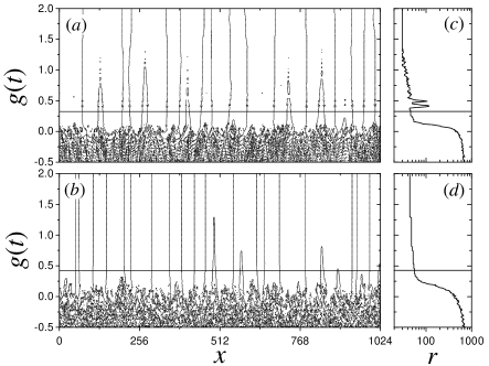
FIG. 1.: Space-time evolution. The positions of crossings of zero are shown as a function of time for underdamped (a) and overdamped (b) dynamics. In (c) and (d) the corresponding numbers of crossings are shown. (Time increases upward.) The horizontal lines correspond to $g=\hat{g}$.

During the evolution preceding $g=\hat{g}$, the cubic term in (2) is small and the linearized equation is a good approximation. It is illuminating to nondimensionalize the linearized equation:

$$\partial^{2}_{T}Y_{T}(x)-\nu\partial^{2}_{x}Y_{T}(x)+2\alpha\partial_{T}Y_{T}(x)$$ (4)

$$=TY_{T}(x)+{\epsilon}{\mu^{-\frac{1}{2}}}\eta(x,t),$$ (5)

$${\rm where} \quad T=\mu^{\frac{1}{3}}t,\quad\alpha=\frac{1}{2}\gamma\mu^{-\frac{1}{3}},\quad\nu=D\mu^{-\frac{2}{3}}.$$ (6)

The dynamics can now be studied in terms of the characteristic time $t=\mu^{-\frac{1}{3}}$ and nondimensional damping $\alpha$. The field $Y_{T}(x)$ satisfying (5) with initial conditions (3) is Gaussian with mean zero at all times. The correlation function, $c(x)={\big{<}Y_{T}(x)Y_{T}(0)\big{>}}$, changes its form and amplitude with time. At any fixed time, there is the following relationship between $c(x)$ and the number of zeros: if $c^{\prime}(0)=0$ then the mean number of zero crossings is a finite number given by [20, 18]

$$\rho(T)=\frac{L}{\pi}\left(-\frac{c^{\prime\prime}(0)}{c(0)}\right)^{\frac{1}{2}}.$$ (7)

Analytical solution of (5) proceeds by separating into independent stochastic differential equations for each of the Fourier coefficients, ${\mbox{\boldmath$y$}}_{T}(k)=L^{-\frac{1}{2}}\int_{0}^{L}Y_{T}(x){\rm e}^{{\rm i}k\frac{2\pi}{L}x}{\textrm{d}}x$, whose time evolution is given by the SDE

$$\partial^{2}_{T}{\mbox{\boldmath$y$}}_{T}(k)+2\alpha\partial_{T}{\mbox{\boldmath$y$}}_{T}(k)=$$ (8)

$$=(T-\kappa^{2}){\mbox{\boldmath$y$}}_{T}(k)+{(2\mu)^{-\frac{1}{2}}}{\epsilon}\,\hat{\mbox{\boldmath$\eta$}}(T,k)$$ (9)

for integer $k$ and where $\kappa^{2}=\nu\,k^{2}(\frac{2\pi}{L})^{2}$ and ${\big{<}\hat{\mbox{\boldmath$\eta$}}(T,k)\hat{\bf\mbox{\boldmath$\eta$}}(T^{\prime},k^{\prime})\big{>}}=\delta_{k,k^{\prime}}\delta(T-T^{\prime})$. Each ${\mbox{\boldmath$y$}}_{T}(k)$ is Gaussian with mean zero [21]. The variance grows exponentially fast for $T-\kappa^{2}+\alpha^{2}>1$:

$${\big{<}{\mbox{\boldmath$y$}}_{T}^{*}(k){\mbox{\boldmath$y$}}_{T}(k)\big{>}}\to\pi\frac{\epsilon^{2}}{\mu}\Phi(T_{0},\alpha,\kappa^{2})\left(T-\kappa^{2}+\alpha^{2}\right)^{-\frac{1}{2}}$$ (10)

$$\times\exp\left(\frac{4}{3}(T-\kappa^{2}+\alpha^{2})^{\frac{3}{2}}-2\alpha(T-\kappa^{2})-\frac{4}{3}\alpha^{3}\right),$$ (11)

where

$$\Phi(T_{0},\alpha,\kappa)={\rm e}^{\frac{4}{3}\alpha^{3}}\displaystyle\int_{T_{0}}^{\infty}{\rm Ai}^{2}({S-\kappa^{2}+\alpha^{2}}){\rm e}^{2\alpha{S}}{\textrm{d}}{S}.$$ (12)

No approximations have been made thus far in the solution of (6). We now consider the implications of the physical picture presented above for the relative values of the parameters. Firstly, for there to be a quasi-adiabatic first regime in the evolution, we require a sufficiently slow sweep: $\mu\ll\tau^{\frac{3}{2}}$ [22]. Secondly, we require a well-defined value of the order parameter, $g=\hat{g}$, marking the end of the second part of the evolution, implying $\epsilon^{2}\ll\mu$ [19].

We adopt the following definition: $\hat{g}=\mu^{\frac{2}{3}}\hat{T}$ where $\hat{T}$ satisfies ${\big{<}Y_{\hat{T}}^{2}(x)\big{>}}=\delta\hat{g}$. (i.e., when $\delta=1$, the first two terms on the RHS of (2) are equally important.) We thus evaluate $\hat{g}$ by solving ${\big{<}Y_{\hat{T}}^{2}(x)\big{>}}=\delta\hat{g}$ where

$${\big{<}Y_{T}^{2}(x)\big{>}}= \frac{1}{L}\sum_{k}{\big{<}{\mbox{\boldmath$y$}}^{*}_{T}(k){\mbox{\boldmath$y$}}_{T}(k)\big{>}}$$ (13)

$$\simeq (\lambda(T))^{-1}(2\pi)^{-\frac{1}{2}}{\big{<}{\mbox{\boldmath$y$}}^{*}_{T}(0){\mbox{\boldmath$y$}}_{T}(0)\big{>}}$$ (14)

and $\lambda(T)=-2\nu\frac{\partial^{2}}{\partial\kappa^{2}}\ln\left({\big{<}{\mbox{\boldmath$y$}}^{*}_{T}(k){\mbox{\boldmath$y$}}_{T}(k)\big{>}}\right)$.

The correlation function is the Fourier transform of ${\big{<}{\mbox{\boldmath$y$}}^{*}_{T}(k){\mbox{\boldmath$y$}}_{T}(k)\big{>}}$. It emerges from the sweep past $g=0$ with the form $c(x)=c(0)\exp(-x^{2}/2\lambda^{2}(\hat{T}))$ [13]. The number of zeros present at $g=\hat{g}$ is thus

$$\rho=\frac{1}{\pi}\frac{L}{\lambda(\hat{T})}.$$ (15)

Our procedure is valid for arbitrary damping. We now examine the underdamped and the overdamped limits, defined by the parameter $\alpha=\frac{1}{2}\gamma\mu^{-\frac{1}{3}}$. The overdamped limit (studied in [13]) is recovered as $\alpha\to\infty$.

The underdamped limit. When $\alpha\to 0$, $\rho$ is only logarithmically dependent on $\alpha$. In this limit $\lambda(T)=2\nu^{\frac{1}{2}}T^{\frac{1}{4}}$, and the integral (12) has the asymptote $\Phi(T_{0},\alpha,\kappa^{2})\to\Phi_{1}|T_{0}-\kappa^{2}|^{\frac{1}{2}}$ [23]. As $T\to\hat{T}$,

$${\big{<}Y_{T}^{2}(x)\big{>}}\to\pi\frac{\epsilon^{2}}{\mu}\Phi_{1}\left(\frac{\tau}{4\pi D}\right)^{\frac{1}{2}}T^{-\frac{3}{4}}\exp({\frac{4}{3}T^{\frac{3}{2}}}),$$ (16)

and $\hat{g}$ satisfies

$$\hat{g}^{\frac{3}{2}}=\frac{3}{4}\mu\ln\left(\frac{\mu}{\pi\epsilon^{2}}(\frac{4\pi D}{\mu\tau})^{\frac{1}{2}}\frac{\delta\hat{g}^{\frac{7}{4}}}{\Phi_{1}}\right).$$ (17)

Immediately before $g=\hat{g}$, the number of zeros (7) is a decreasing function of time, given by

$$\rho(T)=\displaystyle\frac{L}{2\pi}\frac{T^{-\frac{1}{4}}}{\nu^{\frac{1}{2}}}.$$ (18)

The number of zeros present at $\hat{g}$ for $\alpha\to 0$ is

$$\rho(\hat{T})=\frac{L}{2\pi}\frac{\mu^{\frac{1}{3}}}{D^{\frac{1}{2}}}{\left[\frac{3}{4}\ln\left(\frac{\mu}{\pi\epsilon^{2}}(\frac{4\pi D}{\mu\tau})^{\frac{1}{2}}\frac{\delta\hat{g}^{\frac{7}{4}}}{\Phi_{1}}\right)\right]^{-\frac{1}{6}}}.$$ (19)

In the overdamped limit the number of zeros is proportional to $\mu^{\frac{1}{4}}$ [13, 14]. We show that the latter scaling is obtained in the limit $\alpha\to\infty$. Here $\Phi(T_{0},\alpha,\kappa)\to\Phi_{2}\alpha^{-\frac{1}{2}}$ [23] and $\lambda(T)^{2}=2\nu T/\alpha$. Thus

$${\big{<}Y_{T}^{2}(x)\big{>}}=\pi\frac{\epsilon^{2}}{\mu}\frac{\Phi_{2}}{\alpha}(4\pi\nu T)^{-\frac{1}{2}}\exp(\frac{1}{2}\frac{T^{2}}{\alpha})$$ (20)

and $\hat{g}$ satisfies

$$\hat{g}^{2}=\mu\gamma\ln\left(\epsilon^{-2}\gamma\delta(8D\hat{g}^{3})^{\frac{1}{2}}\right).$$ (21)

The number of zeros for overdamped slow passage is

$$\rho(\hat{T})= \displaystyle\frac{L}{2\pi}\frac{(\mu\gamma)^{1/4}}{D^{\frac{1}{2}}}\left[\ln(\epsilon^{-2}\gamma\delta(8D\hat{g}^{3})^{\frac{1}{2}})\right]^{-\frac{1}{4}}.$$ (22)

Equations (19) and (22) are the main results of this Letter: the number of created defects scales with the sweep rate as $\rho\sim\mu^{\frac{1}{4}}$ for the underdamped case and $\rho\sim\mu^{\frac{1}{3}}$ for the overdamped regime. We have performed extensive quantitative comparison with numerical simulations of (2). Two examples are shown in Fig. 2. Our analytical predictions at instant $g=\hat{g}$ are very accurate. Although the exponents can be obtained from dimensional analysis [3, 15], logarithmic corrections produce small deviations in numerically-estimated exponents at finite damping. No evidence has been found for the region of $\rho\sim\mu^{\frac{1}{2}}$ scaling, predicted in [17] from an approximation that replaced (9) by a first-order equation.

Because the number of defects at $\hat{g}$ is typically much larger than the equilibrium density at temperature $\Theta$ [24], their number decreases after $\hat{g}$ as kink-antikink pairs annihilate (see Fig. 1). The smaller the damping, the more rapidly this annihilation proceeds [15]. In Fig. 2 we have also plotted the number of zeros at $g=\tau$. While the number of zeros is reduced, the scaling with $\mu$ seen at $g=\hat{g}$ is preserved.

The crossover between regimes, represented in Fig. 3, takes place when the nondimensional damping $\alpha=\frac{1}{2}\gamma\mu^{-\frac{1}{3}}\simeq 1$. At small damping the dependence of the number of defects on damping is only logarithmic, ($\epsilon^{2}\propto\gamma$). At large damping, $\rho\sim\gamma^{\frac{1}{4}}$.

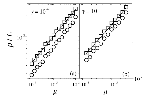
FIG. 2.: Density of zeros for the underdamped (a) and overdamped (b) cases. The lines are the analytical approximations (19) and (22). Averages from numerical simulations of (2) are shown at $g=\hat{g}$ (squares) and $g=\tau$ (circles), with errors of symbol size or smaller. ($D=\tau=1$, $\Theta=5\times 10^{-9}$.)

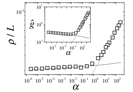
FIG. 3.: From the underdamped to the overdamped regime: density of zeros vs $\alpha$ for fixed $\mu$. Squares are numerical averages. The main plot shows the density of defects at the instant $\hat{g}$ and the analytical predictions for the underdamped (19) and the overdamped (22) regimes. We measured $\hat{g}$ numerically as the instant when ${\big{<}Y^{2}_{\hat{T}}(x)\big{>}}=\frac{1}{2}\hat{g}$. In the inset we plot the value thus obtained vs (17) and (21). ($\mu=10^{-2}$, $D=\tau=1,\Theta=5\times 10^{-9}$.)

Apart from the scaling of the number of defects with $\mu$, a different signature of underdamped dynamics can be seen in in Fig. 1 and Fig. 4: multiple “bounce back” of the number of zeros soon after $g=\hat{g}$. The phenomenon has been reported in simulations of a sudden quench ($\mu=\infty$) [25]. We propose the following interpretation. In a dynamic transition at low damping, domains reach a minimum of a potential well with a finite velocity and therefore oscillate about it for a time. Parts of some domains recross the crest of the instantaneous potential barrier during these oscillations. This yields an estimate of the frequency of the oscillations: $\sqrt{2\hat{g}}$, corresponding to harmonic oscillations about the minimum. In our simulations, two well-defined bumps are typically seen in the number of defects vs time. From this we are able to measure the period, $P$ of the oscillations in the number of zeros; despite the nonlinearity, it is very well approximated by $P=2\pi/\sqrt{2\hat{g}}$ (See Fig. 4).

The procedure carried out in this Letter for the real equation (2) can be applied to other equations exhibiting continuous transitions [13] and in more than one space dimension [13, 16]. The scalings are not sensitive to the particular equations chosen, but they are sensitive to any breaking of the exact $Y\to-Y$ symmetry in the equation of motion.

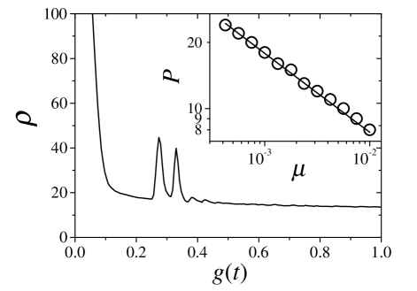
FIG. 4.: “Bounce back”: The number of zeros oscillates after $g=\hat{g}$ for small damping. The graph of $r$ vs time is for $\mu=4\times 10^{-3}$, $\gamma=10^{-4}$, $\epsilon=10^{-6}$ and $D=\tau=1$. The inset plots the period of the oscillations obtained at different values of $\mu$, with $\gamma=10^{-4}$. The straight line is $P=2\pi/\sqrt{2\hat{g}}$ with $\hat{g}$ given by  (17).

In summary, we derive quantitative predictions for the number of defects formed in a symmetry-breaking transition in one space dimension by analyzing the dynamics in the critical region, where the system is out of equilibrium regardless of how slowly the critical parameter is changed. Prefactors are calculated, so no fitting necessary. Underdamped slow passage results in a defect density proportional to $\mu^{\frac{1}{3}}$ and produces characteristic oscillations in the number of zeros. Experiments where liquid Helium is expanded through the Lambda Transition re now reaching the point where quantitative comparisons can be made.

We are grateful for Angel Sanchez’s comments on the manuscript. E. Moro thanks the CNLS for its hospitality.

REFERENCES

- [1] Electronic address: emoro@math.uc3m.es
- [2] Electronic address: grant@lanl.gov
- [3] W.H. Zurek, Nature 317 505-508 (1985); W.H. Zurek, Acta Physica Polonica B 24 1301-1311 (1993).
- [4] P.C. Hendry et al, Nature 315 315-317 (1994); P.C. Hendry et al, Physica B 210 209-214 (1995); C Bäuerle et al, Nature 382 332-334 (1996); V.M.H. Ruutu et al, Nature 382 334-335 (1996); A.J. Gill and T.W.B. Kibble, J. Phys. A 29 4289-4305 (1996); G. Karra and R.J. Rivers, Phys. Lett. B 414 28-33 (1997).
- [5] M.E. Dodd et al, to appear in Phys. Rev. Lett; G. Karra and R.J. Rivers, to appear in Phys. Rev. Lett.
- [6] Paul Mandel and T. Erneux, Phys. Rev. Lett. 53 1818–1820 (1984);
- [7] C. van den Broeck and Paul Mandel, Phys. Lett. A122 36–38 (1987).
- [8] M.C. Torrent and M. San Miguel, Phys. Rev. A 38 245–251 (1988).
- [9] N.G. Stocks, R. Mannella and P.V.E. McClintock, Phys. Rev. A 40 5361–5369 (1989).
- [10] J.W. Swift, P.C. Hohenberg and Guenter Ahlers, Phys. Rev. A 43 6572–6580 (1991).
- [11] G.D. Lythe and M.R.E. Proctor, Phys. Rev. E. 47 3122–3127 (1993).
- [12] J.C. Celet, D. Dangoisse, P. Glorieux, G. Lythe and T. Erneux, Phys. Rev. Lett. 81 975-978 (1998).
- [13] G. D. Lythe, Phys Rev. E 53, R4271 (1996).
- [14] P. Laguna and W.H. Zurek, Phys. Rev. Lett. 78 2519-2522 (1997).
- [15] P. Laguna and W.H. Zurek, xxx.lanl.gov/list/hep-ph/9711411
- [16] Andrew Yates and W.H. Zurek, Phys. Rev. Lett. 80 5477-5480 (1998).
- [17] Jacek Dziarmaga , Phys. Rev. Lett. 81 1551-1553 (1998).
- [18] G. D. Lythe, Anales de Física, 4 55-62 (1998) (xxx.lanl.gov/list/cond-mat/9808242).
- [19] K. Jansons and G.D. Lythe J. Stat. Phys. 90 227-251 (1998).
- [20] K. Ito J. Math. Kyoto Univ. 3-2 207 (1964); R. J. Adler, The Geometry of Random Fields (Wiley, 1981).
-
[21]
The solution of (9) is
is a Wiener process, and are Airy functions.(23) (24) - [22] Richard Haberman, SIAM J. Appl. Math. 37 69-106 (1979); G.J.M. Marée, ibid 56 889-918 (1996).
- [23] The constants used in the calculations are and .
- [24] F.J. Alexander and S. Habib Phys. Rev. Lett. 71 955-958(1993); G. Lythe and S. Habib, in preparation (1998).
- [25] Nuño D. Antunes and Luís M.A. Bettencourt, Phys. Rev. D 55 925-937 (1997).