Self-organized criticality and directed percolation

Abstract

A sandpile model with stochastic toppling rule is studied. The control parameters and the phase diagram are determined through a MF approach, the subcritical and critical regions are analyzed. The model is found to have some similarities with directed percolation, but the existence of different boundary conditions and conservation law leads to a different universality class, where the critical state is extended to a line segment due to self-organization. These results are supported with numerical simulations in one dimension. The present model constitute a simple model which capture the essential difference between ordinary nonequilibrium critical phenomena, like DP, and self-organized criticality.

I introduction

The idea of self-organized criticality (SOC) was introduced to describe the behavior of a class of extended dissipative dynamical systems which naturally evolve to a critical state, consisting of avalanches propagating through the system [1]. From the very beginning it was observed that this new idea has some connections with ordinary critical phenomena [2]. More recently a novel mean field (MF) analysis of SOC was presented, which pointed out similarities between SOC models and models with absorbing states [3]. Directed percolation (DP) [4] is one of the simplest and most recurrent models with absorbing states. Under very general guidelines (locality, scalar variable, etc.) it has been proposed that a wide range of models would fall into DP universality class [4, 5, 6]. Alhouh SOC models do not belong to the DP universality class they have some connection with DP [7, 8, 9].

Recently, Tádic and Dhar have shown that a class of stochastic sandpile model has some analogy with DP [9]. They studied a directed sandpile model in which unstable sites topples with probability $p$. They observed that above a critical threshold $p_{c}$ the system shows SOC, while below the system is not critical. The critical probability was identified with the threshold for DP in a squared lattice and the scaling exponents were obtained in terms of DP exponents. However, they could not give a detailed description of the phase diagram of the model, since their analysis was limited to the SOC regime above $p_{c}$, while the state below $p_{c}$ could not be characterized.

Following the work of Tádic and Dhar we study a class of stochastic sandpile models with undirected toppling rule. As in their model, sites topples with a probability $p$ but now grains are distributed to each nearest neighbor. In order to provide a theoretical description of the model we have generalized the MF theory by Vespignani and Zapperi [3] including the control parameter $p$. In this way we obtain the complete phase diagram of the model. The existence of a critical probability $p_{c}$ and a quasi-stationary state below $p_{c}$ are obtained. Based on the MF analysis and on the evolution rules we argue that the state below $p_{c}$ is similar to DP, but with different boundary conditions. Using this hypothesis we apply the scaling theory developed for DP to the present stochastic sandpile model. Numerical simulations in one dimension support our hypothesis.

The paper is organized as follows. In section II we introduce the dynamical evolution rules for the stochastic version of the Bak-Tang-Wiesenfeld (BTW) model. We perform a single site MF approximation and determine the average densities in the stationary state. It is found that the driving rate $h$ and $p$ are the only control parameters and that the system is critical in the line segment ($h=0^{+}$, $p_{c}\leq p\leq 1$). Then in section III we argument the connection with DP and derive some scaling relations. In order to test our predictions we have performed numerical simulations in one dimension, the main results are presented in section IV. Finally, the summary and conclusions are given in section V.

II MF theory

We study a stochastic sandpile model defined as follows. An integer variable $z_{i}$ (height or energy) is assigned to each site of a $d$-dimensional lattice and energy is added to the system at rate $h$. When a site receives a grain and its energy exceeds a threshold $z_{c}$ then, with probability $p$, it relaxes according to the following rules $z_{i}\rightarrow z_{i}-g$ and $z_{j}\rightarrow z_{j}+1$ at each of $g$ nearest neighbors. Open boundary conditions are assumed. One may call this model non-abelian sandpile model with stochastic rules. The non-abelian behavior makes it different from other stochastic models such as the Manna model [10]. However, we will simply call it stochastic sandpile model.

The first step towards a comprehensive understanding of critical phenomena is provided by mean-field (MF) theory, which gives insight into the fundamental physical mechanism of the problem. Thus, we start analyzing the stochastic sandpile model through a MF approach. With this simple picture we introduce the connection with directed percolation.

The first MF theory for sandpile models was introduced by Tang and Bak [2], and only deterministic toppling rules were considered. Latter Caldarelli et al [11] generalize this MF theory to sandpile models with certain degree of stochasticity in the toppling rules. In particular Caldarelli et al studied sandpile models where $p$ is a function of $z_{i}$, such that $0<p(z)<1$ below the critical threshold $z_{c}$ and $p(z)=1$ above. Their MF theory and further numerical simulations reveals that the stochastic rules, introduced in this way, changes the average of $z$ but does not destroy the critical state [11]. In the sandpile models analyzed by Caldarelli et al $p$ is not a control parameter, its average value is determined by the system dynamics. In these models the system self-organizes itself to a stationary sate, where $\langle p(z)\rangle$ is such that the system remains in a critical state. On the contrary in the stochastic sandpile model considered here $p$ is a control parameter. It is expected that for sufficiently small values of $p$ the critical state will be destroyed. We have therefore to develop a MF theory where $p$ appears explicitly as a control parameter.

Recently Vespignani and Zapperi [3] have introduced a more general framework. As a difference with previous theories, their MF approach is not based in some particular sandpile model but in general considerations which are common to all of them, even extendible to other SOC models [3]. Within this formalism, SOC appears as a special case of nonequilibrium critical phenomena. They have divided the states each site can assume in stable ($s$), critical ($c$), and active ($a$). Stable sites are those that cannot become active by addition of energy, critical sites are those that become active by addition of energy and active sites are relaxing and transfer energy to their neighbors. These definitions becomes very clear in a deterministic sandpile model. For instance (assuming negligible the probability that a site receives two energy grains) sites with $z<z_{c}-1$ are stable, those with $z=z_{c}-1$ are critical and those with $z>z_{c}$ are active. However, in the stochastic model sites with $z\geq z_{c}$ topple with probability $p$. Again sites with $z<z_{c}-1$ are stable since they can never become active after receiving one energy grain. Nevertheless, those with $z\geq z_{c}-1$ have not a well defined state. For instance, sites with $z=z_{c}-1$ may topple after receiving one energy grain and, therefore, they cannot be stable. However, they are not strictly critical because only a fraction $p$ of them will topples after receiving a grain of energy. Hence, in the case of stochastic sandpile models the subdivision in stable, critical and active does not covert all the possible states each site can assume, i.e. $\rho_{s}+\rho_{c}+\rho_{a}<1$.

We divide the states each site can assume in stable ($s$), unstable ($u$), and active ($a$) and denote their average densities by $\rho_{s}$, $\rho_{u}$ and $\rho_{a}$, respectively. The definition of stable and actives sites is the same considered by Vespignani y Zapperi, while unstable sites are now those sites that may become active by addition of energy. Under these definitions, sites with $z<z_{c}-1$ are stable, those with $z=z_{c}-1$ are unstable and those with $z\geq z_{c}$ may be either unstable or active. Only a fraction $p$ of the unstable sites will become active after receiving energy and, therefore, are critical sites, i.e.

$$\rho_{c}=p\rho_{u}.$$ (1)

This equality makes the connection between our MF approach and that of Vespignani and Zapperi [3]. In the deterministic limit $p=1$ there is no distintion between critical and unstable sites.

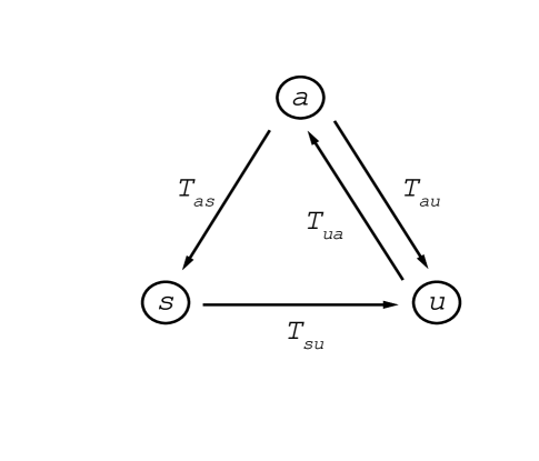
FIG. 1.: Schematic representation of the single site approximation for the stochastic sandpile model. Sites are divided in stable ($s$) unstable ($u$) and active ($s$). $T_{mn}$ are the transition rates for the state $m$ to $n$. Transitions which do not take place are not represented.

To study the dynamics of the stochastic sandpile model we consider the following Markov process for the average densities

$$\frac{\partial}{\partial t}\rho_{n}=\sum_{m\neq n}T_{mn}\rho_{m}-\sum_{m\neq n}T_{nm}\rho_{n},$$ (2)

where $T_{nm}$ are the transition rates from the state $n$ to the state $m$ (see fig. 1). By definition of the model, in one step stable sites never becomes active and unstable sites never become stable, i.e. $T_{sa}=T_{us}=0$. $T_{as}=q$ and $T_{au}=1-q$, where $q$ is the fraction of active sites that becomes stable after relaxing. In deterministic models $q$ may be assumed equal to one [3]. However in stochastic models $z$ may take values large enough compared with $z_{c}$ in such a way that an active site main become unstable after relaxing, i.e. $q<1$. Although an active site with $z\gg z_{c}$ may remain active due to addition of energy this type of transitions are of second order, they can be neglected for $\rho_{a}$ and $h$ small. The transition rates $T_{su}$ and $T_{ua}$ depends on the probability per unit time that a site receives energy. If $\rho_{a}$ and $h$ are small then the probability per unit time that a site receives more than one grain of energy is negligible, and the probability per unit time that a site receive a grain of energy may be approximated by

$$h_{1}=h+(g-\epsilon)\rho_{a},$$ (3)

where $g-\epsilon$ is the effective number of nearest neighbors and $\epsilon$ is the dissipation rate per toppling event, an effective parameter which account for boundary dissipation. If $u$ ($p$) is the fraction of stable (unstable) sites that become unstable (active) after receiving a grain of energy then $T_{su}=uh_{1}$ ($T_{ua}=ph_{1}$). Taking into account these considerations the system of differential eqs. (2) is reduced to

$$\frac{\partial}{\partial t}\rho_{a}=-[1-(g-\epsilon)\rho_{c}]\rho_{a}+\rho_{c}h+O(h^{2},h\rho_{a}),$$ (4)

$$\frac{\partial}{\partial t}\rho_{s}=q\rho_{a}-u(h+g\rho_{a})\rho_{s}+O(h^{2},h\rho_{a}),$$ (5)

together with the normalization condition

$$\rho_{s}+\rho_{u}+\rho_{a}=1.$$ (6)

Notice that, among unstable sites, only the fraction of critical sites $\rho_{c}=p\rho_{u}$ contributes to the system dynamics, the other fraction is only relevant through the normalization condition in eq. (6). The system of equations is completed by the equation of energy balance

$$\frac{\partial}{\partial t}E=(h-\epsilon\rho_{a})L^{d},$$ (7)

where $E$ is the total energy of the system, $hL^{d}$ is the average influx of energy and $\epsilon\rho_{a}L^{d}$ the average outflux of energy.

A Critical state

In the stationary state ($\frac{\partial\rho_{n}}{\partial t}=0$, $\frac{\partial E}{\partial t}=0$) from eqs. (4-7) and (1) we obtain

$$\rho_{a}=\frac{h}{\epsilon},\ \ \ \ \rho_{c}=\frac{1}{g}+O(h),$$ (8)

$$\rho_{u}=\frac{1}{pg}+O(h),\ \ \ \ \rho_{s}=\frac{pg-1}{pg}+O(h),$$ (9)

$$\frac{q}{u}=\frac{pg-1}{p}+O(h).$$ (10)

Comparing this expressions with the ones obtained by Vespignani and Zapperi we observe that the average densities of active and critical sites have the same stationary solutions. The differences appear in the density of stable and unstable sites, which now depends on the new control parameter $p$.

For $1/g\leq p\leq 1$ we have $1/g\leq\rho_{u}\leq 1$, $0\leq\rho_{s}\leq(g-1)/g$ and, therefore, there is not any inconsistency in the stationary solutions obtained above. In this range of $p$, within the MF approach, there is no distinction between the critical state of stochastic and deterministic sandpile models. The model is critical in the double limit $h,\epsilon\rightarrow 0$ and $h/\epsilon\rightarrow 0$ [3] and the susceptibility,

$$\chi=\frac{\partial\rho_{a}}{\partial h}=\frac{1}{\epsilon},$$ (11)

diverges in the critical state. For a small perturbation around the subcritical state $\rho_{a}=h/\epsilon+\Delta\rho_{a}$, $\rho_{c}\approx 1/g$ and from eq. (4) one obtains

$$\Delta\rho_{a}(t)\propto\exp(-\epsilon t/g),$$ (12)

in agreement with the result obtained for deterministic models [3].

From eqs. (11) and (12 one may think that $\epsilon$ is a control parameter of the model. However, if the dissipation takes place only at the boundary then $\epsilon$ will decrease with decreasing system size, because the number of actives sites in the bulk grows faster than the number of active sites at the boundary. Hence, we are just dealing with a finite size effect. The statement the system is not in a critical state is equivalent to the statement there is no critical state in a finite system. If dissipation takes place only at the boundary $\epsilon$ is not a control parameter, it just reflects a finite size effect which at the same time is a necessary condition to obtain a stationary state. In this sense the criticality here is different from the criticality at phase transitions where boundary effects always disappear in the thermodynamic limit [1].

On the contrary, the driving field $h$ is actually a control parameter. Since $h$ must satisfy $h<\epsilon$ and $\epsilon\rightarrow 0$ when $L\rightarrow\infty$ then we must fine tune $h$ to zero in order to obtain criticality in the thermodynamic limit. The time scale separation becomes a necessary condition for criticality. Now if we assumes separation of time scales then $p$ will be the only control parameter of the model. This hypothesis is in general fulfilled in computer simulations, where a new grain of energy is added only once there is no active site.

B Break-down of SOC by stochastic rules

When $0<p<1/g$ the stationary solutions in eqs. (8-10) are no longer valid, because they imply $\rho_{u}>1$ and $\rho_{s}<0$. To understand the origin of this inconsistency let us analyze the variation of $\rho_{u}$ and $\rho_{c}$ with $p$. In the deterministic case $p=1$ there is no distinction between unstable and critical sites, i.e. $\rho_{c}=\rho_{u}=1/g$. However, when $p<1$ critical sites are a fraction $\rho_{c}=p\rho_{u}$ of unstable sites. Hence, since $\rho_{c}=1/g$ in the stationary state, the system has to self-organize itself increasing the average density of unstable sites to $\rho_{u}=1/pg>1/g$ and decreasing the average density of stable sites. But when $p=1/g$ we have $\rho_{u}=1$ and $\rho_{s}=0$ and, therefore, if we continue decreasing $p$ the system cannot provide more unstable sites. Then $\rho_{c}<1/g$ and the stationary solutions in eqs. (8-10) break-downs.

Let us assume that for $0<p<1/g$ the average densities reache an stationary state, which off course cannot be given by eqs. (8-10). From eq. (4) it results that

$$\rho_{a}=\frac{\rho_{c}h}{1-(g-\epsilon)\rho_{c}},$$ (13)

Substituting this expression in eq. (7) one obtains

$$\frac{\partial}{\partial t}E=\frac{1-g\rho_{c}}{1-(g-\epsilon)\rho_{c}}hL^{d}.$$ (14)

According to eq. (1) $\rho_{c}=p\rho_{u}\leq p<1/g$, independent of $\rho_{u}$. Hence, $\frac{\partial E}{\partial t}>0$ and the total energy will increase linearly with time. Moreover, stable sites are those with $z<z_{c}-1$ and, therefore, it is expected that after a time long enough there will be no stable sites. In this quasi-stationary state the energy increases with time and the average densities will take the stationary values

$$\rho_{a}=\frac{hp}{1-(g-\epsilon)p},\ \ \ \ \rho_{c}=p+O(h),$$ (15)

$$\rho_{u}=1+O(h),\ \ \ \ \rho_{s}=0$$ (16)

$$q=0.$$ (17)

Now it is clear that $p$ is a control parameter of the class of stochastic sandpile models analyzed here.

The susceptibility in this region is given by, assuming $\epsilon\ll g$,

$$\chi=\frac{p}{1-pg}.$$ (18)

For a small perturbation around the subcritical state we have $\rho_{a}=\chi h+\Delta\rho_{a}$ and $\rho_{c}\approx p$, then from eq. (4) one obtains, again considering $\epsilon\ll g$,

$$\Delta\rho_{a}(t)\propto\exp[-(1-pg)t].$$ (19)

The critical state breaks-down by the stochastic rules, once $p<p_{c}$. To reach the critical state we have to fine tune $p$. Near the critical threshold $1/g$ the susceptibility $\chi\sim(p_{c}-p)^{-1}$ and the characteristic time $\sim(p_{c}-p)^{-1}$ diverges.

In summary, we found a critical probability $p_{c}$ above which the system is in a SOC state, while it is in a subcritical state below.

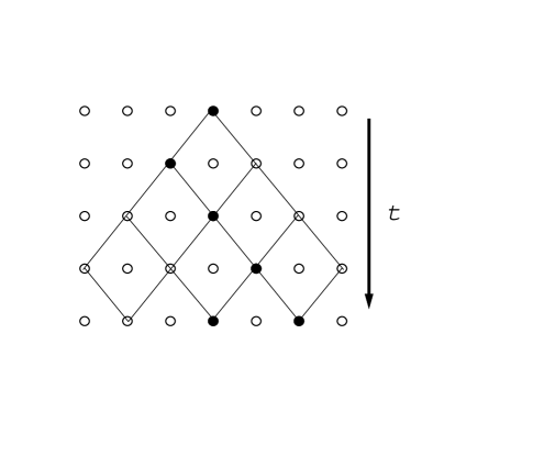
FIG. 2.: Evolution of an avalanche in the stochastic sandpile model. Empty sites are inactive (stable+unstable) and filled sites are active. This figure clearly shows that the avalanche evolves in a directed square lattice, where the probability that a site is present is $\rho_{c}$.

III Scaling theory

$\rho_{c}$ is the probability that a site becomes active after receiving a grain of energy. In the absence of an external field it is the probability that a site becomes active if one of its neighbors was active in the previous step. This problem is equivalent to site directed percolation in $d+1$ dimensions ($d$ spatial dimensios$+$time), $\rho_{c}$ being the probability that a site is present. The only different is found in the boundary conditions, while in DP the system is assumed infinite here we deal with a finite system with open boundaries. This picture is better represented in fig. 2.

A $0<p<p_{c}$

According to the MF theory below the $p_{c}$ there are no stable sites and the fraction of critical sites is given by $\rho_{c}=p$. The evolution rules are thus that of DP. The existence of different boundary conditions may carry as a consequence that some scaling exponents result different, however the nature of the phenomena is the same. For instance, DP near a wall reveals that the correlation length exponents are identical to those obtained in DP in an infinite lattice [12], but other exponents take different values. This is a consequence of the fact that in DP near a wall the avalanches are a subset of the avalanches in DP in an infinite lattice. We thus expect a similar behavior in the stochastic sandpile model below $p_{c}$. In this case, avalanches starting far from the boundary behaves as in DP in an infinite lattice, while avalanches starting near the boundary behaves like the avalanches in DP near a wall. Hence, the correlation lengths and the correlation length exponents are identical to those of DP in an infinite lattice, i.e.

$$\xi_{\bot}\sim(p_{c}-p)^{-\nu_{\bot}},\ \ \ \ \xi_{||}\sim(p_{c}-p)^{-\nu_{||}}.$$ (20)

where $\xi_{\bot}$ and $\xi_{||}$ are the spatial and temporal correlation lengths, respectively, and $\nu_{\bot}$ and $\nu_{||}$ the correlation length exponents.

On the other hand, based on this analogy with DP we write the following scaling relation for the average density of active sites at site $x$ and time $t$, given a site was active in the origin $x=0$ at $t=0$,

$$\rho_{a}(x,t)=t^{\eta-\frac{2}{z}}f\biggl{(}\frac{x^{2}}{t^{2/z}},\frac{t}{\xi_{||}}\biggr{)},$$ (21)

first introduced by Grassberger and de la Torre in the contest of DP [13]. Here $\eta$ is a scaling exponent and $z$ the dynamic scaling exponent, as it is usually defined in the contest of critical phenomena. Moreover, the probability that the avalanche survive up to time $t$ is given by

$$P(t)=t^{-\delta}g\biggl{(}\frac{t}{\xi_{||}}\biggr{)},$$ (22)

where $\delta$ is another scaling exponent. From eq. (21) one can derive other scaling laws for the average number of active sites $n(t)$, the cluster mass $m(t)$ and the mean squared displacement $R^{2}(t)$ at time $t$, resulting

$$\begin{array}[]{l}n(t)=\int d^{d}x\rho_{a}(x,t)=t^{\eta}f_{1}\bigl{(}\frac{t}{\xi_{||}}\bigr{)},\\ m(t)=\int_{0}^{t}dt^{\prime}n(t^{\prime})=t^{1+\eta}f_{2}\bigl{(}\frac{t}{\xi_{||}}\bigr{)},\\ R^{2}(t)=\frac{1}{n(t)}\int d^{d}x\rho_{a}(x,t)x^{2}=t^{2/z}f_{3}\bigl{(}\frac{t}{\xi_{||}}\bigr{)}.\end{array}$$ (23)

The exponent $z$ is not independent, since $t\sim r^{z}$ from eq. (20) one obtains

$$z=\frac{\nu_{||}}{\nu_{\bot}},$$ (24)

and it is therefore identical to that of DP in an infinite lattice. Nevertheless, the exponents $\eta$ and $\delta$ depend on the boundary conditions, as it is observed in DP near a wall [12].

B $p_{c}\leq p<1$

We assume that the scaling laws in eqs. (21-23) are also valid above $p_{c}$, but with $\xi_{||}=\xi_{||}(L)$. In this region the dynamical evolution is independent of $p$ and the characteristic length and time depends only on the lattice size $L$, according to

$$\xi_{\bot}\sim L,\ \ \ \ \xi_{||}\sim L^{z}.$$ (25)

However, as it is shown below, for $p>p_{c}$ the global conservation introduces a constraint between the exponents $\eta$ and $z$.

Let us calculate the average flux of energy $J(r)$ outside an sphere of radius $r$, given a grain of energy was added at the origin $r=0$ at $t=0$. The energy flux is proportional to the gradient of the average density of active sites and, therefore,

$$J(r)\propto r^{2}\int dt\frac{\partial}{\partial r}\rho_{a}(r,t).$$ (26)

Substituting the scaling relation for $\rho_{a}(r,t)$ (21) in this expression it results that

$$J(r)=r^{(1+\eta)z-2}f_{4}\biggl{(}\frac{r}{\xi_{\bot}}\biggr{)}.$$ (27)

Now, conservation implies that $J(r)=1$ for $r<\xi_{\bot}\sim L$ and, therefore,

$$(1+\eta)z=2.$$ (28)

This scaling relation may seem unusual, a more familiar expression is obtained if one calculate the mean avalanche size

$$\langle s\rangle=\int dtn(t)\sim L^{(1+\eta)z}\sim L^{2}.$$ (29)

This scaling relation was previously obtained by Dhar [15] but for a particular sandpile model. We have here demonstrated, using scaling arguments, that it holds for any sandpile model with global conservation.

C Directed models

In the directed stochastic models there is a preferent direction $l$ for the avalanche evolution. This preferent spatial direction may be identified with the time direction in undirected models and then apply the scaling theory developed above. This means that the scaling relations in eqs. (21-23) are also valid for directed models, but now $x$ is a ($d-1$)-dimensional vector in the space of the non-preferent directions and $t$ gives the evolution in the preferent direction $l$.

Another important difference between undirected and directed models is the place where topling take places during the evolution of the avalanche. In the undirected model not only the sites in the avalanche front but also sites inside this front may be active, transfering energy to their neighbors. On the contrary in directed models all active sites are in the avalanche front, i.e. at step $t$ all active sites are in the layer $l=t$. Moreover, actives sites in layer $l$ transfer energy only to those neighbors in layer $l+1$. Hence, in directed models the energy flux take places following the preferent direction, while it take places in all directions in the undirected case.

An inmediate consequence of this difference is that in directed models the average outflux of energy from the $l=t$ to the $l+1$ layer, which is proportional to the average number of active sites in the $l=t$ layer, equals one and, therefore,

$$n(t)\sim 1.$$ (30)

Then, form eq. (23) one obtains that

$$\eta=0.$$ (31)

The energy balance thus leads to a different constraint for the set of scaling exponents $(\eta,z,\delta)$, i.e. the directed model is in a diferent universality class.

IV Numerical simulations and discussion

In order to test our predictions we have performed numerical simulations of the stochastic sandpile model in one dimension. We have investigated both regimes of the phase diagram, the region similar to DP below $p_{c}$ and the SOC region above. In both regions we start with a flat pile, i.e. zero height in all sites, and let the system evolve to the stationary state. Above $p_{c}$ the stationary state is characterized by a constant average energy per site, which was taken as the stationary condition. Below $p_{c}$ the energy increases linearly with time and, therefore, we look for another criterion of stationarity. According to the MF theory in the quasi-stationary state below $p_{c}$ we have $\rho_{u}=1$, which was taken as the stationary condition. In all cases we start measuring after the system reached the stationary state. Average where taken over 10 000 000 avalanches below $p_{c}$ and over 1000 000 avalanches above. Below $p_{c}$ we use the lattice size $L=10240$, which was large enough to avoid finite size effects for the values of $p$ considered. Above $p_{c}$ we use $p=0.708$ and different lattice sizes.

To obtain an estimate of $p_{c}$ we have calculated the correlation lengths in the subcritical state for different values of $p$ and fitted the numerical data to the scaling laws in eq. (20). These magnitudes where computed in the simulations using the following expressions

$$\begin{array}[]{l}\xi_{\bot}^{2}\sim\frac{\sum_{t=0}^{\infty}\sum_{i=0}^{L}(i-i_{0})^{2}\rho_{ai}}{\sum_{t=0}^{\infty}\sum_{i=0}^{L}\rho_{ai}},\\ \\ \xi_{||}\sim\frac{\sum_{t=0}^{\infty}\sum_{i=0}^{L}t\rho_{ai}}{\sum_{t=0}^{\infty}\sum_{i=0}^{L}\rho_{ai}}\end{array}$$ (32)

where $i_{0}$ is the position of the initial active site, $t$ is the number of steps measured in the time scale of the avalanche and $\rho_{ai}=1$ ($\rho_{ai}=0$) in active (unstable) sites.

The log-log plot of the correlation lengths versus $p_{c}-p$ is shown in fig. 4. The best fit to the numerical data was obtained for

$$\begin{array}[]{ll}p_{c}=0.707\pm 0.002,&(0.705485);\\ \nu_{\bot}=1.07\pm 0.03,&(1.0968);\\ \nu_{||}=1.71\pm 0,03,&(1.7338).\end{array}$$ (33)

Enclosed in parenthesis are the series expansion estimates for DP in an infinite lattice reported in [14]. Within the numerical error there is a complete agreement between the values reported here and those of DP.

Then we proceed to determine the exponents $\delta$, $\eta$ and $z$ from the data collapse plots of $P(t)$, $m(t)$ and $R^{2}(t)$, using the scaling laws in eq. (23). The corresponding plots are sown in figs. 4-6. The best data collapse was obtained for

$$\begin{array}[]{ll}\delta=0.18\pm 0.01,&(0.15947);\\ \eta=0.27\pm 0.01,&(0.31368);\\ z=1.59\pm 0.01,&(1.58074);\\ \nu_{||}=1.73\pm 0.01,&(1.7338);\\ (1+\eta)z=2.02\pm 0.02.\end{array}$$ (34)

From the data collapse we have obtained a better estimate for $\nu_{||}$ and, using the scaling relation (24) and the value of $z$ in (34), we obtain the better estimate for $\nu_{\bot}$

$$\begin{array}[]{ll}\nu_{\bot}=1.09\pm 0.02,&(1.0968).\end{array}$$ (35)

As it was expected the critical probability, the correlation length exponents, and $z$ are identical, within the numerical error, to those reported for DP in an infinite lattice, while $\eta$ and $\delta$ results different.

Now let us analyze the numerical simulations in the SOC region $p_{c}\leq p<1$. In this case we can obtain an estimate of the critical probability from the divergence of the average energy per site $\langle E\rangle$ near $p_{c}$. In the SOC region $\langle E\rangle$ reaches a stationary value but it increases with time below $p_{c}$. One thus expect that $\langle E\rangle$ diverges when the system approaches the critical probability from above. We observe that the divergence of $\langle E\rangle$ can be fitted to the power law dependency $\langle E\rangle\sim(p-p_{c})^{-\lambda}$, where $\lambda$ is a scaling exponent. In fig. 7 we have plot the best fit to the numerical data for a lattice size $L=1280$, which was obtained for

$$\begin{array}[]{ll}p_{c}=0.704\pm 0.01,&(0.705485),\end{array}$$ (36)

which is close to the DP value.

Then we proceed to determine the exponents $\delta$, $\eta$ and $z$ from the data collapse above $p_{c}$, using the scaling laws in eqs. (23) and (25). The best data collapse is shown in figs. 8-10 with

$$\begin{array}[]{ll}\delta=0.18\pm 0.01,&(0.15947);\\ \eta=0.28\pm 0.01,&(0.31368);\\ z=1.57\pm 0.01,&(1.58074);\\ (1+\eta)z=2.01\pm 0.02\end{array}$$ (37)

From the comparison of these values with those in eq. (34) we conclude that the scaling exponents $\delta$, $\eta$ and $z$ are the same above and below $p_{c}$. Moreover, the scaling relation in eq. (28) is in both cases satisfied, although it was demonstrating only for $p>p_{c}$. Hence, there are only three independent scaling exponents, $\nu_{\bot}$, $\nu_{||}$ and $\delta$, while $z$ and $\eta$ can be determined using the scaling relations in eqs. (24) and (28). The correlation length exponents are identical to those of DP in an infinite lattice while $\delta$ depends on the boundary conditions and, therefore, changes the universality class.

V Summary and conclusions

We have obtained, through a MF analysis, the phase diagram of the stochastic sandpile model. There is a critical probability $p_{c}$ above which the system is in a SOC state, where the correlation lengths diverge in the thermodynamic limit. Below $p_{c}$ the system is subcritical, it is characterized by a finite susceptibility which diverges when the critical state is approached. While the stationary state in the SOC state is characterized by a well defined average energy per lattice site the subcritical state is not completely stationary, since the average energy per lattice size increases linearly with time. It was then corroborated that the global conservation is a necessary condition to obtain SOC in sandpile models.

Using scaling arguments it was demonstrated that in the subcritical region the stochastic sandpile model is similar to DP, but with different boundary conditions. On the other hand, the scaling theory in the SOC state reveals that global conservation introduces a constraint among the scaling exponents, generalizing previous results obtained for particular sandpile models. We have provided a general demonstration of the scaling law $\langle s\rangle\sim L^{2}$.

Numerical simulations have corroborated the predictions of the MF and scaling theory. The correlation length exponents and the critical probability were found, within the numerical error, identical to the estimates for DP. However, the existence of different boundary conditions and conservation law carries as a consequence that other exponents result different, changing the universality class.

We must emphasize that the stochastic sandpile model is not just another cellular automaton showing SOC, but a very nice example to understand the differences and similarities between SOC and ordinary nonequilibrium critical phenomena. The comparison of the phase diagram of this model with that of DP reveals the essential property of SOC, the insensitive to changes in certain ”control” parameter, which is off course no more a control parameter. While the critical state in DP is restricted to a point in the phase diagram, in the stochastic sandpile model it is extended through a line segment.

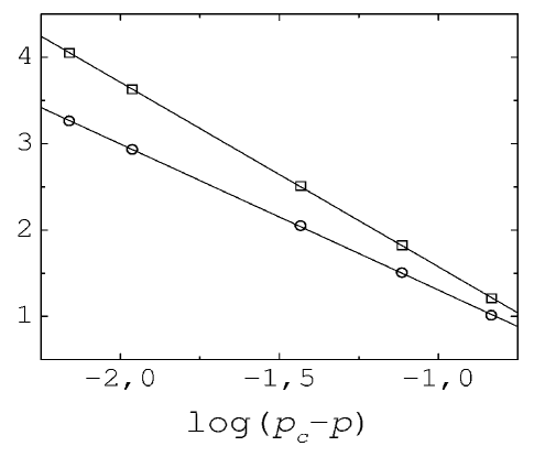
FIG. 3.: The correlation lengths $\log\xi_{\bot}$ (squares) and $\log\xi_{||}$ (circles) as a function of $p$ in the subcritical state. The lines are linear fits to the log-log plot.

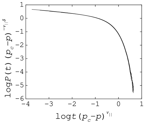
FIG. 4.: Data collapse plot for $P(t)$ in the subcritical state for $p=0.670$, 0.688, 0.696 and 0.700.

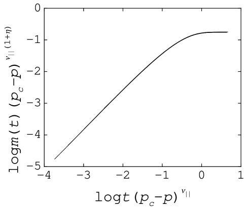
FIG. 5.: Data collapse plot for $m(t)$ in the subcritical state for $p=0.670$, 0.688, 0.696 and 0.700.

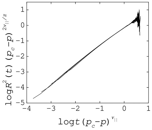
FIG. 6.: Data collapse plot for $R^{2}(t)$ in the subcritical state for $p=0.670$, 0.688, 0.696 and 0.700.

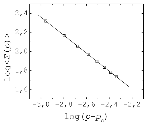
FIG. 7.: Average energy per lattice site as a function of $p$ in the SOC state. The continuous line is a linear fit in the log-log scale.

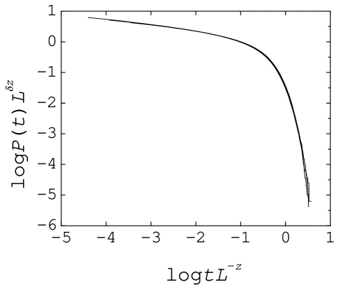
FIG. 8.: Data collapse plot for $P(t)$ in the SOC state for $L=160$, 320 and 640.

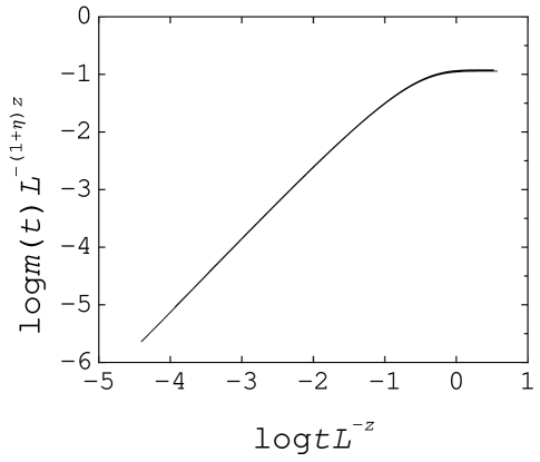
FIG. 9.: Data collapse plot for $m(t)$ in the SOC state for $L=160$, 320 and 640.

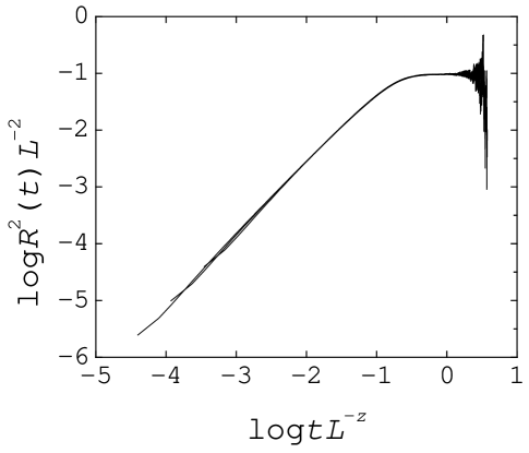
FIG. 10.: Data collapse plot for $R^{2}(t)$ in the SOC state for $L=160$, 320 and 640.

REFERENCES

- [1] P. Bak. C. Tang, and K. Wiesenfeld, Phys. Rev. Lett. 59, 381 (1987).
- [2] C. Tang and P. Bak, Phys. Rev. Lett. 60, 2347 (1988); C. Tang and P. Bak, J. Stat. Phys. 51, 797 (1988).
- [3] A. Vespignani and S. Zapperi, Phys. Rev. Lett. 78, 4793 (1997); Phys. Rev. E 57, 6345 (1998).
- [4] P. Grassberguer, J. Stat. Phys. 79, 12 (1995); and references therein.
- [5] H. K. Janssen, Z. Phys. B 42, 151 (1981).
- [6] P. Grassberger, Z. Phys. B 47, 365 (1982).
- [7] Z. Olami, I. Procaccia, and R. Zeittav, Phys. Rev. E 49, 1232 (1994).
- [8] P. Grassberger, Phys. Lett. A 200, 277 (1995).
- [9] B. Tádic and D. Dhar, Phys. Rev. Lett. 79, 1519 (1997).
- [10] S. S. Manna, Physica A 179, 249 (1991).
- [11] G. Caldarelli, Physica A 252, 295 (1997).
- [12] J. W. Essam, A. J. Guttmann, I. Jensen, and D. Tanlakishani, J. Phys. A 29, 1619 (1996).
- [13] P. Grassberger and A. de la Torre, Ann. Phys. 122, 373 (1979).
- [14] I. Jenssen, J. Phys. A 29, 7013 (1996).
- [15] D. Dhar, Phys. Rev. Lett. 64, 1613 (1990).