[

Quantized Röntgen Effect in Bose–Einstein Condensates

Abstract

A classical dielectric moving in a charged capacitor can create a magnetic field (Röntgen effect). A quantum dielectric, however, will not produce a magnetization, except at vortices. The magnetic field outside the quantum dielectric appears as the field of quantized monopoles.

today

]

Bose–Einstein condensation is believed to be at the heart of superfluidity and superconductivity [1]. Formulated in the most elementary model, a large number of either neutral atoms or electrically charged Cooper pairs condense and constitute a macroscopic wave function. Flowing Cooper pairs form electric currents that in turn act on magnetic fields, and the magnetic properties of superconductors cause the phenomenon of electric superconductivity itself [2]. On the other hand, superfluids, i.e. Bose–condensed atoms, are electrically neutral, yet they are polarizable and form a dielectric medium.

Can quantum dielectrics generate magnetic fields? Imagine the setup depicted in Fig. 1.

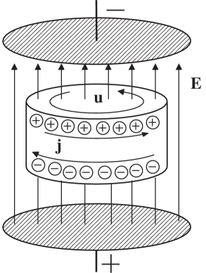
FIG. 1.: Sketch of Röntgen’s experiment. A dielectric moves with the velocity profile ${\bf u}$ in a charged capacitor. The co–moving surface charges of the polarized medium form a current ${\bf j}$ and thus generate a magnetic field.

A capacitor polarizes the dielectric layer between the plates. When the medium is moving, co–moving surface charges appear as electric currents and produce a magnetic field. In 1888 W.C. Röntgen [3] observed the effect for the first time (before he discovered X-rays). Röntgen employed a rotating glass disc (and also a rubber disc) as a moving dielectric medium in a charged capacitor, and he noticed a feeble deflection of a magnetic needle. More recently the interest in Röntgen’s effect [4] has revived [5, 6, 7, 8], because the effect gives rise to a novel topological phase of neutral atoms.

What happens when Röntgen’s glass disc is replaced by a quantum dielectric (a Bose–Einstein condensate)? We show in this paper that only vortices of the quantum liquid can generate a magnetization. Moreover, the magnetic field outside a thin quantum–dielectric layer appears as the field of a set of magnetic monopoles with magnetic charges that sit in the vortex cores. The monopoles turn out to be quantized [9] with a magnetic flux of

$$\Phi_{n}=\frac{hn}{mc^{2}}\,\chi\,U\,.$$ (1)

Here $U$ denotes the applied voltage, $\chi$ is the susceptibility, $m$ is the atomic mass, $c$ denotes as usual the speed of light, and $hn$ is an integer multiple of Planck’s constant $h=2\pi\hbar$. The quantized Röntgen effect of a single vortex is very small, yet modern “magnetic needles” (SQUIDs) might be able to detect it. Let us present our case beginning with a general theory of condensed atoms that move in electromagnetic fields. Then we turn to the quantum version of Röntgen’s experiment.

Moving atoms in electromagnetic fields.— Any magnetic effect has its root in relativity. Let us first consider a classical atom that moves with velocity $\mathbf{v}$ in a given electromagnetic field. The neutral yet polarizable atom responds to the electric field in its restframe. According to relativity, this field contains an electric and a magnetic component of the electromagnetic field in the laboratory frame. In lowest order of $v/c$ we use the mechanical Lagrangian [6] (in SI units)

$$L_{A}=\frac{m}{2}v^{2}+\frac{\alpha}{2}E^{2}-\alpha{\bf v}({\bf E}\times{\bf B})\,.$$ (2)

The constant $\alpha$ denotes the electrical polarizability of the atom. Due to relativity the Poynting vector ${\bf E}\times{\bf B}$ of the electromagnetic field couples to the atom’s motion in precisely the same way as the vector potential couples to a charged particle.

To study the motion of an atomic de–Broglie wave $\psi$ in an electromagnetic field, we follow the canonical procedure. First, we find the momentum ${\bf p}$ and the Hamiltonian $H$ of the classical atom,

$${\bf p} = \frac{\partial L}{\partial{\bf v}}=m{\bf v}-\alpha({\bf E}\times{\bf B})\,,$$ (3)

$$H = {\bf pv}-L=\frac{1}{2m}({\bf p}+\alpha{\bf E}\times{\bf B})^{2}-\frac{\alpha}{2}E^{2}\,,$$ (4)

and then we write down the Schrödinger equation

$$i\hbar\frac{\partial\psi}{\partial t}=\frac{1}{2m}(-i\hbar\nabla+\alpha{\bf E}\times{\bf B})^{2}\psi-\frac{\alpha}{2}E^{2}\psi\,.$$ (5)

In the case of a Bose–Einstein condensate, $|\psi|^{2}$ describes the density of the condensed atoms (in mean–field theory [10]). The condensate moves with the velocity profile

$${\bf u}=\frac{1}{m}(\hbar\nabla S+\alpha{\bf E}\times{\bf B})\,,\qquad\psi=|\psi|e^{iS}\,,$$ (6)

because ${\bf u}$ satisfies the continuity relation

$$\frac{\partial|\psi|^{2}}{\partial t}+\nabla(|\psi|^{2}{\bf u})=0\,.$$ (7)

Condensed atoms interact by collisions. In order to form a stable condensate for large numbers of particles, the atoms must repell each other [10]. We model atomic collisions by adding a Gross–Pitaevskii term $g|\psi|^{2}\psi$ [10] with positive $g$ to the right–hand side of the Schrödinger equation (5). The atomic repulsion tends to smooth out density variations over the healing length $\hbar/\sqrt{2gm|\psi|^{2}}$ [10]. To prevent the condensate from spreading out to infinity, an external potential $V$ must balance out the inter–atomic repulsion. The potential $V$ models a trap or simply the interactions with the walls of a container. Finally, we condense our description of moving atoms in electromagnetic fields into the Lagrangian density

$${\mathscr{L}}_{A} = \frac{i\hbar}{2}(\psi^{\ast}\dot{\psi}-\dot{\psi^{\ast}}\psi)+\left(\frac{\alpha}{2}E^{2}-\frac{g}{2}\,|\psi|^{2}-V\right)|\psi|^{2}$$ (8)

$$- \frac{1}{2m}(i\hbar\nabla+\alpha{\bf E}\times{\bf B})\psi^{\ast}\cdot(-i\hbar\nabla+\alpha{\bf E}\times{\bf B})\psi\,.$$ (9)

One verifies easily that the Euler–Lagrange equations of ${\mathscr{L}}_{A}$ lead to the Gross–Pitaevskii equation (including electromagnetic and external interactions).

So far we have described atoms that move in given electromagnetic fields. For understanding the condensate as a dielectric medium we must study the effect of the atoms on the fields. For this we add to ${\mathscr{L}}_{A}$ the Lagrangian density ${\mathscr{L}}_{F}$ of the free electromagnetic field (in SI units), and we arrive at the total Lagrangian

$${\mathscr{L}} = {\mathscr{L}}_{F}+{\mathscr{L}}_{A}\,,$$ (10)

$${\mathscr{L}}_{F} = \frac{\varepsilon_{0}}{2}(E^{2}-c^{2}B^{2})\,,$$ (11)

$${\bf E} = -(\dot{\bf A}+\nabla U),\quad{\bf B}=\nabla\times{\bf A}\,,$$ (12)

where ${\bf A}$ denotes the vector potential. Then we minimize the total action $\int{\mathscr{L}}\,d^{4}x$ with respect to $\bf A$ and $U$, and obtain

$$\nabla\times{\bf E} = -\frac{\partial{\bf B}}{\partial t}\,,\qquad\nabla{\bf B}=0\,,$$ (13)

$$\nabla\times{\bf H} = +\frac{\partial{\bf D}}{\partial t}\,,\qquad\nabla{\bf D}=0\,,$$ (14)

with

$${\bf D} = \varepsilon_{0}(1+\chi){\bf E}+\varepsilon_{0}\chi{\bf u}\times{\bf B}\,,$$ (15)

$${\bf H} = \varepsilon_{0}c^{2}{\bf B}+\varepsilon_{0}\chi{\bf u}\times{\bf E}\,,$$ (16)

and

$$\varepsilon_{0}\chi=\alpha\,|\psi|^{2}\,.$$ (17)

These are Maxwell’s equations for the electromagnetic field in the presence of a moving dielectric medium [11, 12], written in lowest order of $u/c$. The medium has a susceptibility $\chi$ given by Eq. (17) and moves with the velocity profile ${\bf u}$ of Eq. (6). Consequently, moving atoms form indeed a classical dielectric medium (like Röntgen’s glass disc). On the other hand, where are the quantum effects?

Quantized Röntgen effect.— Consider a charged capacitor that contains a movable quantum dielectric, see Fig. 1. We will use cylindrical coordinates $(\varrho,\varphi,z)$ to describe the physical situation. We require that no motion occurs in $z$ direction and that the susceptibility $\chi$ (the density $|\psi|^{2}$) be uniform in planes of constant $z$. A $z$–dependance of $\chi$ accounts for the finite thickness of the quantum dielectric layer. Furthermore, matter and fields are assumed to be stationary, i.e. all time derivatives vanish. We derive from Maxwell’s equations (14) combined with the constitutive equations (16)

$$\nabla{\bf H} = \varepsilon_{0}[{\bf E}(\nabla\times\chi{\bf u})-\chi{\bf u}(\nabla\times{\bf E})]$$ (18)

$$= \varepsilon_{0}{\bf E}(\nabla\times\chi{\bf u})\,.$$ (19)

From the very beginning (2) we have restricted our attention to effects that occur in the lowest order of $v/c$. Hence we can replace the electric field ${\bf E}$ in Eq. (19) by the ${\bf E}$–field in zeroth order (without Röntgen effect), i.e. by

$${\bf E}=E(z){\bf e}_{z},\qquad E(z)=\frac{E_{0}}{1+\chi(z)}\,.$$ (20)

The curl component of $\chi{\bf u}$ that stems from $\chi^{\prime}(z)$ is orthogonal on ${\bf e}_{z}$ and therefore on ${\bf E}$. Consequently,

$$\nabla{\bf H}=\varepsilon_{0}\chi{\bf E}(\nabla\times{\bf u})\,.$$ (21)

The source of the magnetic field is the curl of the velocity profile projected onto the applied electric field. Two components contribute to the velocity, as is shown in Eq. (6). One stems from the canonical momentum $\hbar\nabla S$ and the other from the Poynting vector ${\bf E}\times{\bf B}$. Let us estimate the influence of the Poynting–vector contribution on the generation of ${\bf H}$. We find that

$$\left|\frac{\alpha}{m}{\bf E}\times({\bf E}\times{\bf B})\right| \leq \frac{\alpha}{m}E^{2}|{\bf B}|=\frac{\chi\varepsilon_{0}E^{2}}{mc^{2}|\psi|^{2}}|{\bf H}|$$ (22)

$$\ll |{\bf H}|\,,$$ (23)

because in realistic capacitors the electrostatic energy density $\varepsilon_{0}E^{2}/2$ is much smaller than $mc^{2}|\psi|^{2}$ (and otherwise pair production would occur). Consequently, only the curl of $(\hbar/m)\nabla S$ generates the ${\bf H}$–field. However, the curl of a gradient uses to vanish, with the remarkable exception of vortices.

A moving dielectric will not produce a magnetic field, except at localized vortices with the velocity profile (in cylindrical coordinates)

$${\bf u}=\frac{\hbar}{m}\nabla S\,,\qquad S=-n\varphi\,,\qquad n\in\mathbb{Z}\,,$$ (24)

because for a vortex (24) the curl of ${\bf u}$ is proportional to a delta function. Vortices are quantized, since the wave functions $|\psi|\,\exp(iS)$ are supposed to be single–valued. Let us calculate the ${\bf B}$ field of an isolated vortex. We derive from Maxwell’s equations (14) and from the constitutive equations (16)

$$\nabla\times{\bf B}=\frac{1}{c^{2}}\nabla\times({\bf E}\times\chi{\bf u})\equiv\frac{1}{\varepsilon_{0}c^{2}}{\bf j}_{R}\,.$$ (25)

We utilize the continuity equation (7) of the medium and the zeroth–order ${\bf E}$–field of Eq. (20) to arrive at

$$\nabla\times{\bf B}=\frac{E_{0}}{c^{2}}\frac{\hbar n}{m\varrho}{\bf e}_{\varphi}\frac{\partial}{\partial z}\left[\frac{\chi(z)}{1+\chi(z)}\right]\,.$$ (26)

We see that the Röntgen current ${\bf j}_{R}$ is induced by the electric field ${\bf E}$ and is concentrated near the surfaces of the quantum dielectric where $\chi(z)$ varies significantly. We obtain the solution

$${\bf B} = \int\limits_{-\infty}^{+\infty}f_{n}(z_{0}){\bf B}_{0}\,dz_{0}\,,$$ (27)

$${\bf B}_{0} = -\nabla\frac{1}{\sqrt{\varrho^{2}+(z-z_{0})^{2}}}-\frac{2}{\varrho}\delta(z-z_{0}){\bf e}_{\varrho}\,,$$ (28)

$$f_{n}(z) = -\frac{\hbar n}{2mc^{2}}\chi(z)E(z)\,,$$ (29)

because ${\bf B}_{0}$ satisfies

$$\nabla\times{\bf B}_{0} = 0-\frac{2}{\varrho}{\bf e}_{\varphi}\delta^{\prime}(z-z_{0})\,,$$ (30)

$$\nabla{\bf B}_{0} = 4\pi\delta^{3}({\bf x}-z_{0}{\bf e}_{z})-2\cdot 2\pi\delta^{3}({\bf x}-z_{0}{\bf e}_{z})=0\,.$$ (31)

Figure 2 shows the magnetic field lines that are bent by a vortex in a charged capacitor. Inside the dielectric layer the vortex’ core attracts the field lines that leave the medium at a well localized spot of roughly the thickness of the layer. In fact, we obtain in the limit of a thin layer

FIG. 2.: Quantum Röntgen effect. Consider a uniform layer of a quantum dielectric (Bose–Einstein condensate) with a single vortex. The medium is polarized and generates a magnetic field. The field is rotationally symmetric, and the figure shows a two–dimensional cut of the magnetic field lines. Inside the layer (between $z=-1$ and $z=+1$ in arbitrary units) field lines are attracted and directed to the vortex’ core (at the origin) where the lines leave the medium. In our simplified model the magnetic field lines close at infinity.

$${\bf B}\sim\frac{\Phi_{n}}{4\pi r^{2}}{\bf e}_{r}-\frac{2f_{n}(z)}{\varrho}{\bf e}_{\varrho}\,,$$ (32)

written using spherical coordinates with $r^{2}=\varrho^{2}+z^{2}$. Outside the medium the vortex appears as a three–dimensional magnetic monopole with a magnetic flux of

$$\Phi_{n}=4\pi\int\limits^{+\infty}_{-\infty}f_{n}(z)dz=-\frac{hn}{mc^{2}}\int\chi{\bf E}\,d{\bf r}\,.$$ (33)

For a uniform layer with a constant susceptibility $\chi$ inside and a vanishing $\chi$ outside we arrive at the simple result (1) that was mentioned in the introductory part of this paper. Inside the medium the ${\bf B}$ field appears as a two–dimensional monopole field that supplies the 3D monopole with field lines.

Can one measure the effect?— Despite the breathtaking progress in the Bose-Einstein condensation of alkali atoms since the pioneering breakthrough [13], superfluid helium is probably still the best candidate for a quantum dielectric medium. Helium is light with a rest mass of roughly four proton masses and the liquid is relatively dense with a susceptibility $\chi=0.052$. Using these numbers we obtain a quantized flux $\Phi_{n}$ per voltage $U$ of $n\cdot 5.7\cdot 10^{-26}\,[{\rm Tm^{2}/V}]$. The flux is quite small yet the magnetic field is most probably measurable using nano–fabricated SQUIDs, taking advantage of the fact that the field stems from an extremely well localized spot. In fact, for a nanometer–size helium film we obtain a magnetic field (25) of a few femtotesla per applied volt at a single vortex with $n=1$, and this field seems to be measurable. One could also think of using much thinner helium layers that will lead to stronger magnetic fields. A helium film can be 0.1 monolayers thick and still be superfluid (where a monolayer has a thickness of $3.6\cdot 10^{-10}\,{\rm m}$). The quantized Röntgen effect could be applied to detect vortices in flowing helium films and to study their interactions. The generated magnetic field may serve as a sensor for vorticity. As we have seen, vortices of quantum dielectrics give rise to interesting magnetic fields — 3D monopole fields outside and 2D monopole fields inside the layer, and we find it worthwhile to study these fields experimentally. Superfluid helium is probably the best material to observe the quantized Röntgen effect with existing techniques, but it is also conceivable to employ optically trapped alkali or other Bose–Einstein condensates.

Summary.— A moving quantum dielectric sandwiched between two charged capacitor plates will not produce a magnetic field, except at vortices. Here the generated field outside the medium appears as the field of a magnetic monopole with the quantized flux (1) and a magnetic charge that is localized in the vortex’ core.

Our paper complements the recent effort [5, 6, 7, 8] in employing the Röntgen interaction of traveling dipoles for novel topological effects. In this case the electromagnetic field forms a vortex of the Poynting vector and acts on moving atoms. In our case, the atomic condensate acts on the fields in the same way as a moving dielectric medium. Quantum mechanics, however, restricts the properties of the medium. We believe that our approach of regarding a Bose–Einstein condensate as a dielectric medium will open a new research road in the fascinating field of quantum gases. Subtle quantum effects may lead to new surprises.

We are grateful to E. Anderson, P. J. Bardroff, M. V. Berry, M. Fontanelle, D. B. Haviland, M. Krusius, P. Öhberg, M. Revzen, W. Schleich, S. Stenholm, M. Wilkens, and A. F. G. Wyatt for helpful discussions. U. L. thanks the Alexander von Humboldt Foundation and the Göran Gustafsson Stiftelse for support. P. P. was supported by the research consortium Quantum Gases of the Deutsche Forschungsgemeinschaft.

REFERENCES

- [1] D. R. Tilley and J. Tilley, Superfluidity and Superconductivity, (Adam Hilger, Bristol, 1990).
- [2] L. D. Landau and E. M. Lifshitz, Electrodynamics of Continuous Media, (Pergamon, Oxford, 1984).
- [3] W. C. Röntgen, Ann. Phys. Chem. 35, 264 (1888).
- [4] M. Babiker, E. A. Power, and T. Thirunamachandran, Proc. Roy. Soc. A 332, 187 (1973); M. Babiker, J. Phys. B 17, 4877 (1984); C. Baxter, M. Babiker, and R. Loudon, Phys. Rev. A 47, 1278 (1993); V. Lembessis, M. Babiker, C. Baxter, and R. Loudon, ibid. 48, 1594 (1993); M. Wilkens, ibid. 47, 671 (1993); 48, 570 (1994).
- [5] M. Wilkens, Phys. Rev. Lett. 72, 5 (1994).
- [6] H. Wei, R. Han, and X. Wei, Phys. Rev. Lett. 75, 2071 (1995).
- [7] Theoretical problems of Ref. [6] were discussed in C. R. Hagen, Phys. Rev. Lett. 77, 1656 (1996); H. Wei, R. Han, and X. Wei, ibid. 1657 (1996); U. Leonhardt and M. Wilkens, Europhys. Lett. 42, 365 (1998); J. Audretsch and V. D. Skarzhinsky, Phys. Lett. A 241, 7 (1998); U. Leonhardt, ibid. (submitted).
- [8] An experiment to measure the topological phase of neutral atoms [6] is under construction, T. Pfau (private communication).
- [9] The quantization of our quasi–monopoles should not be confused with the quantization of Dirac’s magnetic monopoles, P. A. M. Dirac, Proc. Roy. Soc. A133, 60 (1931).
- [10] See e.g. the review article F. Dalfovo, S. Giorgini, L. P. Pitaevskii, and S. Stringari, cond–mat/9806038.
- [11] See §76 of Ref. [2]. Note that we employ SI units instead of the Gaussian ones used in Ref. [2].
- [12] See also Chapter 4 of J. Van Bladel, Relativity and Engineering, (Springer, Berlin, 1984).
- [13] M. H. Anderson et al., Science 269, 198 (1995); C. C. Bradley et al., Phys. Rev. Lett. 75, 1687 (1995); K. B. Davis et al., ibid. 75, 3969 (1995).