A microscopic model for mixed surfactant vesicles

Abstract

A microscopic model which has proven useful in describing amphiphilic aggregates as inhomogeneities of a fluid is extended here to study the case of a two component surfactant mixture. We have chosen an effective interaction between the amphiphiles that mimics the mixture of cationic–anionic surfactants. In agreement with experiments, and other theoretical approaches, we find regions where spherical vesicles are stable, with a well defined radius. The experimental dependence of the radius on the chemical environment is also qualitatively reflected in our model.

¹Departamento de Física Teórica de la Materia Condensada, Universidad Autónoma de Madrid, E-28049 Madrid, Spain

²Instituto Nicolás Cabrera, Universidad Autónoma de Madrid, E-28049 Madrid, Spain

³Instituto de Ciencia de Materiales, Consejo Superior de Investigaciones Científicas, E-28049 Madrid, Spain

I Introduction

The structure and thermodynamical properties of fluid membranes composed of amphiphilic molecules are of prime scientific and technological importance. In particular the formation of vesicles has received very close attention due to their pharmacological applications (microencapsulation) and their use as models for biological membranes. Usually, large vesicles are formed by intense mechanical shear (sonication), but they are a metastable phase which disappears after a time of hours or days. Only recently has been found spontaneous formation of long-lived vesicles, suggesting that the vesicles could be an equilibrium state of the system [1, 2, 3, 4, 5, 6]. We considerer here binary surfactant mixtures, which are the main body of the experimental systems with this behavior [1, 2, 3, 4], although there are also a few observations for systems with only one surfactant component [5, 6]. Note that the thermodynamic status of these systems is still an open question. The spontaneous vesicles may be truly at equilibrium or they may be a long-lived transient state to a lamellar phase [7]. It has also been argued that the existence of vesicles, and their size distribution, may result from the edge energy and the dynamics of growth [8]. Else, as an equilibrium property, that they arise from the entropy associated with the position and shape of the vesicles [9], rather than to the existence of a preferential curvature for an isolated vesicle.

We may distinguish two main kinds of two-component systems in which spontaneous formation of vesicles appear. In the first, the two amphiphiles have different self-assembly behavior. One of them (a phospholipid molecule) is quasi insoluble in water and tends to form lamellar phases, while the other (a surfactant molecule) is soluble in water up to a critical surfactant concentration and then tends to form micelles. One example of these systems is the mixture of octylglucoside and phosphatidylcholine [1]. The second possibility is that both surfactants have similar self-assembly properties and its vesicular behavior is due to the nature of the interaction between the two species. The main examples of these systems are mixtures of two ionic surfactants, with oppositely charged head groups. The mixture of the two types, in the solution, may form spontaneous vesicles, which would not appear in pure solutions of either of the surfactants. Many experimental observations have been reported on these catanionic systems [2, 3, 4]. In this work, we will only study this later kind of vesicular system, and search for the possible existence of spontaneous curvature, and typical vesicle sizes, based on the thermodynamic stability of single vesicles. We will neglect the effects of polydispersity and shape entropy. We will use the words vesicle and membrane indistinctly to refer to bilayer aggregates; in each case, we will make clear whether we are referring to a closed vesicle or a planar membrane.

Recently Safran et al [10, 11] have treated this problem under the hypothesis that the existence of spontaneous curvature for the vesicles is associated with the breaking of the composition symmetry between the two molecular layers in the membrane. In a semiempirical Landau theory, the free energy of a spherical membrane of radius $R$ is written in terms of its curvature, ${\sc c}=1/R$, and the relative concentrations of each species, $A$ and $B$, in each molecular layer, $x_{i}^{A}=1-x_{i}^{B}$, with $i=1,2$, for the two layers of the bilayer membrane. These relative concentrations are described by an overall relative concentration

$$\psi=\frac{1}{4}(x_{1}^{A}+x_{2}^{A}-x_{1}^{B}-x_{2}^{B})=\frac{1}{2}(x_{1}^{A}+x_{2}^{A}-1),$$

which takes values $\pm 1$ for pure membranes (of $A$ or $B$ molecules) and is zero for a membrane with symmetric concentrations of $A$ and $B$. The second order parameter is a transverse relative concentration,

$$\phi=\frac{1}{2}(x_{2}^{A}-x_{1}^{A})=\frac{1}{2}(x_{1}^{B}-x_{2}^{B}),$$

which measures the asymmetry between the two layers in the membrane, being zero for symmetric membranes. Since all the $x_{i}^{\xi}$ have to be between $0$ and $1$, $\phi$ is constrained to be between $1/2-|\psi|$ and $-1/2+|\psi|$. For planar membranes, the free energy should be symmetric in $\phi$, but there may be spontaneous symmetry breaking when the membrane goes through a phase transition which preferentially segregates the two species on different sides of the bilayer membrane. For vesicles with ${\sc c}\neq 0$ there is a difference between the inner and the outer layer, which breaks the symmetry of the free energy with respect to $\phi$. The presence of a coupling term proportional to ${\sc c}\phi$ favors the formation of curved vesicles with asymmetric composition ${\sc c}\propto\phi$. The resulting phase diagram exhibits a line of second-order transitions between the lamellar and vesicle phases, with the highest critical temperature corresponding to the system with a symmetric global composition $\psi=0$. At lower temperature, there is a tricritical point where the transition becomes first order. Although these semiempirical theories give a very interesting and clarifying picture of these systems, they are parameter dependent and have a simplified functional dependence of the free energy. To check the validity of the later and to relate the parameters to molecular interactions requires microscopic theories. Safran et al [10, 11] discussed the use of their model to explain the energetic stabilization of two-component vesicles, for mixtures of amphiphiles which differ only in their polar head groups. The curvature is associated with the different concentrations of the two components in the inner and outer monolayer of the membrane. Also, they assume that this different concentration between layers is promoted by a interaction which gives phase separation in the same layer. As a consequence, they choose a repulsive interaction between the two different components.

We have recently developed a simple microscopic model [12, 13] for the study of aggregates of monocomponent amphiphilic molecules in water, which makes possible a consistent thermodynamic treatment of the system by taking account of the coexistence with the dilute solution of amphiphiles. The model considers only the positional and orientational distribution of the amphiphiles, ignoring internal degrees of freedom. The effective interactions between the amphiphiles is described by a potential which includes the interaction with the water (so that water molecules need not be explicitly taken into account). This minimal model gives a qualitatively correct global phase diagram for aggregates with planar, spherical, and cylindrical symmetry. The elastic constants obtained are in good agreement with experimental results. Depending of the interaction potential, the model exhibits coexistence between a solution of free molecules, micelles, and planar membranes. This monocomponent model does not give spontaneous curvature for any interaction potential and therefore the spherical vesicles are always unstable when compared with the micelles or with the planar membranes.

The goal of the present work is to extend the above model to the study of stability and phase behavior of two–component vesicles. As in the study of the elastic constants [13], the self consistent thermodynamic treatment, i.e. the thermodynamic equilibrium between the solution of amphiphiles and the vesicles, shows interesting restrictions on the possible values of the parameters used in semiempirical Landau theories. In order to exclude other possible sources of spontaneous curvature, we use a model in which the interactions are fully symmetric. Thus, the pure component membrane made with $A$ molecules is exactly equivalent to the pure $B$ membrane. In experimental systems with catanionic surfactants this symmetry is not perfect, i.e. the properties of the two types of pure component systems are not equal, but still they are much more similar than the properties of the surfactant mixture.

II Density functional model

In this section we extend our previous approach [12] to the case of two different components, which we label $\xi=A$, $B$. The model is based on the description of the microscopic or mesoscopic molecular aggregates in water, as inhomogeneous density distributions, treated within the density functional formalism. We use an approximation to the exact Helmholtz free energy density functional, $F[\rho^{\xi}]$, applied to a very simple molecular interaction model. As the amphiphilic molecules are much larger that the water molecules, our previous approach described the interaction between them by a potential which represents an effective, water-mediated interaction ( and so, water molecules need not be explicitly taken into account in the model). The head part of an amphiphilic molecule attracts water much more strongly that the lipid tail. This fact produces an effective repulsion between the head of a molecule and any other molecule (regardless of the orientation of the latter because it displaces the water). We consider the amphiphiles as uniaxial molecules without internal degrees of freedom, other than the orientation of the head-tail direction, which is described by a unit vector ${\bf\hat{u}}$ along the molecular axis. Let us consider a $\xi$–molecule at ${\bf r}_{1}$, with orientation ${\bf\hat{u}_{1}}$, and a $\xi^{\prime}$–molecule at ${\bf r}_{2}$ with orientation ${\bf\hat{u}_{2}}$. The effective pairwise potentials between them, with the proper features, may be written as $\Phi^{\xi,\xi^{{{}^{\prime}}}}({\bf r}_{2}-{\bf r}_{1},\hat{\bf u}_{1},\hat{\bf u}_{2})=\Phi_{0}^{\xi,\xi^{{{}^{\prime}}}}(r_{21})+\Phi_{a}^{\xi,\xi^{{{}^{\prime}}}}({\bf r}_{21},\hat{\bf u}_{1},\hat{\bf u}_{2})$. The isotropic part $\Phi_{0}$ only depends on the distance between the molecular centers, $r_{21}=|{\bf r}_{21}|=|{\bf r}_{2}-{\bf r}_{1}|$, and the anisotropic part, $\Phi_{a}$, may be written as a general expansion in spherical harmonics. As we have argued in our previous papers on monocomponent systems [12, 13], we need only include the terms which do not couple the orientation of the two molecules. The general form is

$$\Phi_{a}^{\xi,\xi^{{{}^{\prime}}}}({\bf r}_{21},\hat{\bf u}_{1},\hat{\bf u}_{2}) = \sum_{i=1}^{\infty}\Phi_{i}^{\xi,\xi^{{{}^{\prime}}}}(r_{21})\times$$ (2)

$$\left[P_{i}(\hat{\bf u}_{1}\cdot\hat{\bf r}_{21})+P_{i}(-\hat{\bf u}_{2}\cdot\hat{\bf r}_{21})\right],$$

where ${\bf\hat{r}}_{21}={\bf r}_{21}/r_{21}$ and $P_{i}(x)$ are the Legendre polynomials. This restriction of the model interactions has the advantage that minimization with respect to orientational degrees of freedom can be done analytically.

The Helmholtz free energy density functional may be approximated by

$$F[\rho^{A}({\bf r},\hat{\bf u}),\rho^{B}({\bf r},\hat{\bf u})]=F_{0}[\rho^{A}({\bf r}),\rho^{B}({\bf r})]$$ (3)

$$+k_{B}T\sum_{\xi=A,B}\int d{\bf r}_{1}d\hat{\bf u}_{1}\rho^{\xi}({\bf r}_{1})\alpha^{\xi}({\bf r}_{1},\hat{\bf u}_{1})\log(4\pi\alpha^{\xi}({\bf r}_{1},\hat{\bf u}_{1}))$$ (4)

$$+{1\over 2}\sum_{\xi=A,B}\sum_{\xi^{{{}^{\prime}}}=A,B}\int d{\bf r}_{1}d\hat{\bf u}_{1}d{\bf r}_{2}d\hat{\bf u}_{2}\rho^{\xi}({\bf r}_{1},\hat{\bf u}_{1})\rho^{\xi^{{{}^{\prime}}}}({\bf r}_{2},\hat{\bf u}_{2})\Phi_{a}^{{\xi}\xi^{{{}^{\prime}}}}({\bf r}_{21},\hat{\bf u}_{1},\hat{\bf u}_{2}).$$ (5)

The first term is the density functional for the isotropic reference fluid; it depends on the density distributions, $\rho^{\xi}({\bf r})$. The second term is the rotational entropy and the third one is the mean field contribution of the anisotropic interactions; both depend on the position and molecular orientation distributions, $\rho^{\xi}({\bf r},\hat{\bf u})$, with $\alpha^{\xi}({\bf r},\hat{\bf u})\equiv\rho^{\xi}({\bf r},\hat{\bf u})/\rho^{\xi}({\bf r})$.

As stated in the introduction we are interested in the study of a mixture of surfactants with similar self-assembly properties, so that the formation of vesicles is due to the interaction between the two species. Within this scheme, it is logical to assume that the $A$–$A$ interaction is equal to the $B$–$B$ one, but different from the $A$–$B$ interaction: $\Phi_{a}^{AA}=\Phi_{a}^{BB}\neq\Phi_{a}^{AB}$. We have fixed the shape of the potentials following the experience gained in the monocomponent case. We consider that the isotropic potential energy $\Phi_{0}^{\xi\xi^{{{}^{\prime}}}}(r)$ is essentially repulsive, since an attractive contribution would produce the unrealistic segregation of water-rich and amphiphilic-rich bulk fluid phases. As the simplest choice, we use a repulsive isotropic interaction consisting of a hard sphere (HS) potential, $\Phi_{\mathrm{hs}}^{\xi\xi^{{{}^{\prime}}}}(r)$. By symmetry, the sphere diameter, $d_{\mathrm{hs}}$, is taken to be identical for the two species. We choose this hard sphere diameter as the unit length and $k_{B}T=\beta^{-1}$ as the unit of energy. For the anisotropic potential we have considered a single form, irrespective of the species involved, changing only their prefactors. The first coefficient function of the anisotropic potential given by eq 1 was taken to be an empty-core Yukawa potential,

$$\Phi_{1}^{\xi\xi^{{{}^{\prime}}}}(r)={K^{\xi\xi^{{{}^{\prime}}}}\over r}exp(-\lambda\ (r-d_{\mathrm{hs}})),$$

for $r\geq d_{\mathrm{hs}}$, and null inside the hard core, $r<d_{\mathrm{hs}}$. The next coefficient function in eq 1 is taken to be proportional to the first, $\Phi_{2}^{\xi\xi^{{{}^{\prime}}}}(r)=q\Phi_{1}^{\xi\xi^{{{}^{\prime}}}}(r)$, and all the rest coefficient functions are neglected. Based in our previous work, we will consistently use $\lambda d_{\mathrm{hs}}=2$ and $q=0.5$. The latter choice is made so that the monocomponent planar membrane will be stable with respect to the micelles, in the range of couplings we consider. In contrast, when $q\leq 0.3$ the micellar structures are more stable. Thus, the model only has two unprefixed adimensional parameters: $\tilde{K}=\beta K^{AA}/d_{\mathrm{hs}}=\beta K^{BB}/d_{\mathrm{hs}}$, the measure of the amphiphilic character of the pure surfactants, and the ratio of like/dislike energies, given by $\epsilon=K_{AB}/K_{AA}$. Note that within this model we could study the first kind of vesicle systems, in which the two surfactant have different self-assembly behavior, considering, e.g., $q=0$ for the surfactant component and $q=0.5$ for the phospholipid molecules. This study is left for a later work.

For a given temperature, $T$, and chemical potentials, $\mu^{A},\mu^{B}$, we have to search for local minima of the grand potential energy, with respect to the distribution functions $\rho^{\xi}({\bf r},\hat{\bf u})$. Due to our simplified choice of anisotropic interactions, the minimization with respect to $\alpha^{\xi}({\bf r},\hat{\bf u})$ may be carried out analytically. Thus,

$$\alpha^{\xi}({\bf r},{\bf\hat{u}})=\frac{1}{z^{\xi}}\exp\left({\sum_{\xi^{{{}^{\prime}}}=A,B}{\bf a}^{\xi\xi^{{{}^{\prime}}}}{\bf\hat{u}}+\sum_{\xi^{{{}^{\prime}}}=A,B}{\bf\hat{u}}^{T}\cal{B}^{\xi\xi^{{{}^{\prime}}}}{\bf\hat{u}}}\right),$$

where the constants $z^{\xi}$ ensure the normalization condition of $\alpha^{\xi}$, i.e. $\int\alpha^{\xi}({\bf r},{\bf\hat{u}})d{\bf\hat{u}}=1$. For each possible value of $\xi$ and $\xi^{{{}^{\prime}}}$, ${\bf a}^{\xi\xi^{{{}^{\prime}}}}$ is a vector arising from the first coefficient function of the anisotropic potential and $\cal{B}^{\xi\xi^{\prime}}$ is a tensor associated to the second coefficient. Their values are given by:

$${\bf a}^{\xi\xi^{{{}^{\prime}}}}({\bf r}_{1})=-\beta\int d{\bf r}_{2}\rho^{\xi^{{{}^{\prime}}}}({\bf r}_{2})\Phi^{\xi\xi^{{{}^{\prime}}}}_{1}(|{\bf r}_{12}|){\bf\hat{r}}_{12}$$

and

$${\cal B}^{\xi\xi^{{{}^{\prime}}}}({\bf r}_{1})=-\beta\int d{\bf r}_{2}\rho^{\xi^{{{}^{\prime}}}}({\bf r}_{2})\Phi^{\xi\xi^{{{}^{\prime}}}}_{2}(|{\bf r}_{12}|)\frac{3{\bf\hat{r}}_{12}\otimes{\bf\hat{r}}_{12}-{\bf\bar{I}}}{2},$$

where ${\bf\bar{I}}$ is the identity matrix and $\otimes$ is a direct product. For planar and spherical symmetries the expressions simplify and we only have to consider the modulus of ${\bf a}^{\xi\xi^{{{}^{\prime}}}}({\bf r})$ and the largest eigenvalue of ${\cal B}^{\xi\xi^{{{}^{\prime}}}}({\bf r})$; these we will call $a^{\xi\xi^{{{}^{\prime}}}}({\bf r})$ and $b^{\xi\xi^{{{}^{\prime}}}}({\bf r})$, respectively.

By substitution of the above into eq 2 we get a free energy density functional, which is already minimized with respect to the molecular orientations:

$$F[\rho^{A}({\bf r}),\rho^{B}({\bf r})] = \min\{F[\rho^{A}({\bf r},\hat{\bf u}),\rho^{A}({\bf r},\hat{\bf u})]\ \}_{\alpha}=$$ (6)

$$= \Delta F_{\mathrm{hs}}[\rho({\bf r})]+k_{B}T\sum_{\xi=A,B}\int d{\bf r}_{1}\rho^{\xi}({\bf r}_{1})\log(\rho^{\xi}({\bf r}_{1})-1)$$ (7)

$$- \sum_{\xi=A,B}\int d{\bf r}\rho^{\xi}({\bf r})\log\left(Q^{\xi}({\bf r})\right),$$ (8)

where

$$Q^{\xi}({\bf r})=\frac{1}{2}\int_{-1}^{1}dx\exp\left(\sum_{\xi^{{{}^{\prime}}}=A,B}\left\{a^{\xi\xi^{{{}^{\prime}}}}({\bf r})P_{1}(x)+b^{\xi\xi^{{{}^{\prime}}}}({\bf r})P_{2}(x)\right\}\right),$$

and $\rho({\bf r})=\rho^{A}({\bf r})+\rho^{B}({\bf r})$ is the total density. In our calculations the interaction part $\Delta F_{\mathrm{hs}}[\rho({\bf r})]$ of the hard sphere free energy is approximated by a well tested non-local density functional [14].

In absence of external potentials, this density functional always has a stationary grand-potential energy for a homogeneous density distribution $\rho^{\xi}({\bf r})=\rho_{0}^{\xi}$, for which ${\bf a}^{\xi\xi^{{{}^{\prime}}}}({\bf r})$ and ${\cal B}^{\xi\xi^{{{}^{\prime}}}}({\bf r})$ vanish. This state represents a mixture of surfactant molecules with random orientations, which in our mean field description is equivalent to a hard spheres mixture. The densities of this homogeneous solution are used to control the chemical potentials, $\mu^{\xi}$, in our search for inhomogeneous density distributions. In this case the expression for the chemical potentials is

$$\beta\mu^{\xi}=\log(\rho_{0}^{\xi})+\beta\mu_{\mathrm{hs}}(\rho_{0}),$$

where $\mu_{\mathrm{hs}}(\rho_{0})$ is the excess (over the ideal) chemical potential of a hard sphere fluid at a total density $\rho_{0}$.

For low values of $\mu^{\xi}$ (and $\rho_{0}^{\xi}$), the homogeneous phase represents a dilute solution of amphiphilic molecules in water and we may find other local minima of the grand potential energy,

$$\Omega[\rho^{A}({\bf r}),\rho^{B}({\bf r})]=F[\rho^{A}({\bf r}),\rho^{B}({\bf r})]\ -\mu^{A}\ \int d{\bf r}\ \rho^{A}({\bf r})-\mu^{B}\ \int d{\bf r}\ \rho^{B}({\bf r}),$$ (9)

for non-uniform density distributions, which represent the different types of molecular aggregates.

III Results

We are interested in the vesicle-planar membrane phase diagram. In this phase diagram we must require that the aggregates are in chemical equilibrium with the dilute surrounding solution of free molecules (which we call “the bulk”), i.e. that they be local minima of eq 4. Beyond of this condition of local stability, we have to seek a global stability, which means that the excess grand-potential energy of the aggregate, with respect to the bulk solution, has to be exactly zero. This is a strong requirement, which comes from the consistent thermodynamic treatment of the model, and it sets important restrictions on the possible structures of the aggregates.

Although the minimization of eq 4 can be carried out exactly, we have calculated the coexistence line within a parameterized family of variational density profiles, which improves the computational efficiency without important changes in the results [12]. With this approach, it is easy to impose a well–defined mean radius to the structure, whose inverse is the curvature, ${\sc c}$. In order to search for vesicles, we impose spherical symmetry and minimize the free energy of our system with respect to the density profiles. As vesicles are characterized by two peaks corresponding to the two monolayers, a useful parameterization of each of the two density profiles is achieved by two Gaussians superimposed on an uniform background; hence we will need four of them. The minimization is made with respect to the twelve parameters that characterize the Gaussians: widths $\alpha_{i}^{\xi}$ (four parameters), surface densities of the monolayers $\eta_{i}$ (two parameters), relative compositions $x_{i}^{\xi}$ (two parameters), radius $R_{v}^{\xi}$ (two parameters), and distances between layers $d^{\xi}$ (two parameters). In practice, the radius and the distance between layers are almost always equal for both species. Thus, our density distributions are given by:

$$\rho^{\xi}(R) = \rho_{0}^{\xi}+\eta_{1}x_{1}^{\xi}\left(\frac{\alpha_{1}^{\xi}}{\pi}\right)^{1/2}\exp[-\alpha_{1}^{\xi}(R-(R_{v}^{\xi}-d^{\xi}))^{2}]$$ (10)

$$+ \eta_{2}x_{2}^{\xi}\left(\frac{\alpha_{2}^{\xi}}{\pi}\right)^{1/2}\exp[-\alpha_{2}^{\xi}(R-(R_{v}^{\xi}+d^{\xi}))^{2}]$$ (11)

Here, the $x_{i}^{\xi}$ have the same meaning as in ref 10 and 11, and from them we get directly the variables $\phi$ and $\psi$ defined above.

In Figure 1 we show a typical profile obtained with our model for a spherical vesicle. As can be seen, the profile exhibits two layers of amphiphiles with different composition. In this case the concentration of the minority component $B$ is higher in the outer layer than the inner one and the majority component has an opposite behavior. The orientational profiles are very similar to those obtained in the monocomponent case, being saturated and of opposite sign at the monolayers, thus indicating the different orientations of the molecules.

FIG. 1.: Density profiles for a spherical vesicle at equilibrium, with bulk densities $\rho_{0}^{A}=9\ 10^{-7}$, and $\rho_{0}^{B}=3.4\ 10^{-14}$. Dashed line: density of the majority component $\rho^{A}(R)$. Dot–dashed line: density of the minority component $\rho^{B}(R)$. Solid line: full density profile $\rho(R)$. The interaction potential parameters are $\tilde{K}=10$ and $\epsilon=1.4$. The hard sphere diameter is used to provide the units of distance and density.

As first step we study the phase diagram for planar membranes, taking the vesicle radius, $R_{v}$, to infinity. In Figure 2 we present the line of stability for $\epsilon=1.4$, with $\tilde{K}$ being a function of the total density of surfactant in the bulk solution, $\rho_{0}=\rho^{A}_{0}+\rho^{B}_{0}$, for different values of the difference in the chemical potential of the two species, $\beta\Delta\mu=\log(\rho^{A}_{0}/\rho^{B}_{0})$. In the region below each line, the membranes have $\Delta\Omega>0$, i.e. they are unstable and would dissolve in the water. In the upper region $\Delta\Omega<0$, so that the planar membranes grow taking particles from the bath; then the bulk density is depleted to the coexistence value. The main qualitative change, with respect to the pure surfactant membranes comes from the possibility that membranes have a spontaneous symmetry breaking, which gives them asymmetric composition $\phi\neq 0$. This effect happens as a second-order phase transition, at positions on the coexistence curves (the places marked by the arrows in Figure 2) which help in stabilizing the membranes and lower down the lines in the figure. It is important to remark that this segregation is only possible when there is a reasonable amount of the two species, $A$ and $B$, in the membrane. But the effect is obtained even if the bulk solution has strong majority of one of the species. The bilayer membrane is able to concentrate the minority species by many orders of magnitude of its bulk concentration, and then it may segregate preferentially in one of the the two molecular layers. Obviously, once the planar membrane undergoes the phase transition, there is no symmetry reason to avoid spontaneous curvature of the membrane into a closed vesicle. This is the coupling, between the composition asymmetry and spontaneous curvature, which acts to stabilize the vesicles proposed by Safran et al [10, 11], and we may now analyze it within our microscopic model. The main difference here is that in our model this coupling is fixed by the molecular interactions and by the requirements of global thermodynamic stability, instead of being a free parameter (assumed constant) in the effective Landau free energy.

FIG. 2.: Equilibrium lines in a $\log(\rho_{0})$ – $\tilde{K}$ phase diagram for planar membranes, with $\epsilon=1.4$. The dashed line gives the monocomponent limit $\Delta\mu\rightarrow\infty$. The full lines show the coexistence line for several values of $\Delta\mu=4,6,8$, from bottom to top. The arrows mark the points where $\phi$ becomes different from zero.

The first result of the consistency within our microscopic model, in which we have assumed perfect symmetry between the two types of surfactant, is that the spontaneous curvature should vanish not only for symmetric membranes, with $\phi=0$, but also for membranes with preferential segregation of each surfactant in one of the layers, $\phi\neq 0$, but with equal global concentration of the two species, $\psi=0$. Thus, in the Landau free energy the coupling term has to go like ${\sc c}\phi f(\psi)$ (where f is an odd function of $\psi$ that vanishes at $\psi=0$), instead of being a constant times ${\sc c}\phi$, as taken in ref 11. In real catanionic mixtures, this symmetry between the two components is not perfect, but still they are probably closer to our ideally symmetric model than to the the model with constant $f(\psi)$.

The simplest Landau free energy we may write, with this requirement, is

$$f=T_{1}\phi^{2}+T_{2}\psi^{2}+a_{1}\phi^{4}+a_{2}\psi^{4}+a_{12}\phi^{2}\psi^{2}+\kappa[{\sc c}^{2}-2\gamma{\sc c}\phi\psi]-2\psi\Delta\mu,$$

where we have approximated the function $f$ by a linear function of $\psi$. The coefficients $a_{1}$, $a_{2}$, $a_{12}$, $\kappa$ and $\gamma$ are assumed to be positive constants. $T_{1}$ and $T_{2}$ correspond to the reduced critical temperatures, which are negative below critical points for the order parameters $\phi$ and $\psi$ in the planar membranes (${\sc c}=0$). In the effective free energy used by MacKintosh and Safran [11], the two temperatures $T_{1}$ and $T_{2}$ are taken to be identical, which would correspond to independent phase transitions in each monolayer, with the preferential segregation of each type of surfactants on uncorrelated patches in the two sides of the bilayer. In our case (with the term $\gamma{\sc c}\phi\psi$ instead of $\gamma{\sc c}\phi$) we require $T_{1}<T_{2}$, so that the parameter $\phi$ goes through a phase transition when $T_{1}$ changes sign while $T_{2}$ is always positive. In the case of catanionic surfactants our assumption is apparently easier to justify, given long ranged attraction between molecules of different types, than the hypothesis of MacKintosh and Safran, which requires an effective attraction between molecules of the same species in order to have segregation at each monolayer.

The minimization with respect to the curvature leads to an effective free energy

$$f=T_{1}\phi^{2}+T_{2}\psi^{2}+a_{1}\phi^{4}+a_{2}\psi^{4}+(a_{12}+3\kappa\gamma^{2})\phi^{2}\psi^{2}-2(\Delta\mu)\psi.$$ (12)

There is a line of critical temperatures $T_{c}(\Delta\mu)$, starting at $T_{c}(0)=T_{1}$, below which both ${\sc c}$ and $\phi$ become nonzero. In Figure 3, we present a sketch of equilibrium curvature of vesicles, at fixed $T$, as a function of the $\Delta\mu$ in the free energy given by eq 6 —dot–dashed line— and by the free energy analyzed by MacKintosh and Safran [11] —dashed line—. The qualitative difference is the behavior at $\Delta\mu=0$ associated to the symmetry of our model. In both cases, the general prediction of the Landau theory is that there may exist a tricritical point at which the transition becomes first order, through the coupling with $\psi$. However, in our microscopic model, we have not found any situation in which the effective parameters in eq 6 lead to a first-order transition. The requirement of thermodynamic equilibrium with the bulk imply strong limitations in the possible values of these parameters.

FIG. 3.: Curvature of the vesicle ${\sc c}$ as a function the difference between chemical potentials $\Delta\mu$. Solid line: our microscopic theory along of the equilibrium curve, with $\tilde{K}=10$ and $\epsilon=1.4$. Dashed line: schematic curve obtained with a Landau theory assuming a coupling ${\sc c}\phi$ between the curvature and the membrane composition. Dot–dashed line: As for the previous curve, but now assuming a coupling ${\sc c}\phi\psi$.

If we compare the empirical form of the free energy given by the eq 6 with the numerical result for our microscopic model, we find that the fit of the free energy, as a function of curvature, to a second-order polynomial is always very accurate. Thus confirming a Helfrich–like picture in which an expansion of the free energy to two second-order in the curvature is carried out. The fit also allows us to safely extrapolate to the infinite radius (zero curvature) limit. However, the dependence of the free energy on the composition of the membranes, i.e. with the variables $\psi$ and $\phi$, is quite beyond the truncated Taylor expansion used in eq 6. The actual results for the curvature, also shown in Figure 3 —solid line—, show a richer dependence of the spontaneous curvature with $\Delta\mu$.

To obtain the global phase diagram for curved structures in our model, we have taken as a starting point the results for the planar membrane ${\sc c}=0$, presented in Figure 2. In this way, for $\epsilon=1.4$, we choose a value of the temperature, for instance $\tilde{K}=10$, so that for any value of $\Delta\mu$ there is a unique value of the total bulk density of the surfactants, $\rho_{o}$, such that the planar membrane has zero surface tension, $\Delta\Omega(\rho_{0},{\sc c}=0)=0$. When the dependence of $\Omega$ with respect to the vesicle curvature, ${\sc c}$, is included we obtain results like those in Figure 4 for $\Delta\mu=18.718$ (curve (a)) and $17.692$ (curve (b)). In the first case, the global minimum is precisely at ${\sc c}=0$ and the membrane does not have spontaneous curvature. In case (b) the spontaneous curvature lowers the value of $\Delta\Omega$ below zero. The global thermodynamic equilibrium in this latter case requires a change of the bulk density $\rho_{0}$, from $1.1761\ 10^{-6}$ to $1.1756\ 10^{-6}$ to recover the condition $\min[\Delta\Omega(\rho,{\sc c})]=0$, as shown in curve (c). Now, repeating the procedure for any values of $\tilde{K}$, we could draw the phase diagram for curved structures (vesicles), but it is not necessary because is equal to the obtained for planar membranes since the shift of the bulk coexistence density is too small to be distinguishable in the scale of Figure 2.

FIG. 4.: Excess free energy per particle, $\Delta\omega=\Delta\Omega/\Delta N$, versus curvature for $\tilde{K}=10$ and $\epsilon=1.4$. a) Planar membrane ${\sc c}=0$ at coexistence, with $\log(\rho_{0})=-13.5837$ and $\Delta\mu=18.718$; b) Vesicle ${\sc c}\neq 0$ beyond coexistence, with $\log(\rho_{0})=-13.6533$ and $\Delta\mu=17.692$; c) Vesicle ${\sc c}\neq 0$ at coexistence, with $\log(\rho_{0})=-13.6537$ and $\Delta\mu=17.692$. Notice how slight the correction is between the parameters in b) and c).

In the Figure 5 we present another view of the coexistence line for bilayer vesicles, in terms of the concentration ratio and of the total bulk density (always for $\tilde{K}=10$ and $\epsilon=1.4$). The full line gives the concentration ratio measured in the bulk $log(\rho^{A}_{0}/\rho^{B}_{0})$ (which is precisely $\beta\Delta\mu$), moving along a horizontal line would correspond to change the total concentration of surfactant but keeping the bulk ratio between the two species. Bulk dilutions on the left of the full line would be stable, while on the right of the line they would form bilayer membranes. This coexistence line also can be represented in term of the composition of the membrane instead of the bulk composition. So, in the same figure, the dashed lines give the ratio between the two surfactant species in the membranes, within our parametrization $\rho^{\xi}_{m}=\eta_{1}x^{\xi}_{1}+\eta_{2}x^{\xi}_{2}$. The ratio between the two species is directly given by the parameter $\psi$, $\rho^{A}_{m}/\rho^{B}_{m}=(1-2\psi)/(1+2\psi)$. As already noted for the planar case, the condensation of the surfactant on the membrane produces a very important change in the relative concentrations of the two surfactant species, given by the vertical separation between the full and the dashed lines in the Figure 5. A bulk dilution in which the species $B$ is in clear minority (e.g. $\Delta\mu=\log(\rho_{0}^{A}/\rho_{0}^{B})\sim 10$) coexists with vesicles in which the two components have comparable concentrations ($\log(\rho_{m}^{A}/\rho_{m}^{B})\sim 1$).

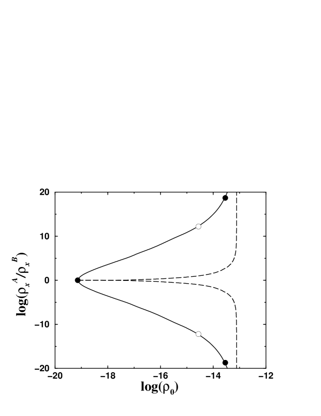
FIG. 5.: Equilibrium curve for the vesicles as a function of the relative concentration and the total bulk density $\log(\rho_{0})$. For the solid line, the relative concentration is measured in the bulk $\log(\rho_{0}^{A}/\rho_{0}^{B})=\Delta\mu$. Alternately for the dashed line, the relative concentration is measured in the membrane $\rho^{A}_{m}/\rho^{B}_{m}=(1/2-\psi)/(1/2+\psi)$. The energy parameters are $\tilde{K}=10$ and $\epsilon=1.4$. Notice how slowly the membrane ratio grows as compared with the bulk one, reflecting the ability of vesicles to concentrate the minority component. As explained in the text, the circles mark the places where ${\sc c}$ reaches zero.

The results for the spontaneous curvature of the vesicles along the coexistence line are given by the full line in Figure 3, to be compared with the results of the simple Landau theories. For $|\Delta\mu|>18.7$ the membrane is symmetric (and planar), since the minority component is too scarce to allow the segregation phase transition. This situation corresponds to the behavior on the right hand side of Figure 5, in which both the bulk and the membrane tend asymptotically to the one-component case. As we lower the values of $|\Delta\mu|$ the transition takes place, there appears spontaneous curvature of the vesicles, and the composition asymmetry of the two layers develops rapidly. But this transition requires the incorporation into the membrane of a significant amount of the minority component, which pushes the membranes towards more symmetric composition, $\rho^{A}_{m}\approx\rho^{B}_{m}$, and it is represented by the dashed lines going to zero, on the left of Figure 5. In accordance with the symmetry arguments presented above, the membranes become flat again at the symmetric mixture ($\Delta\mu=0$ and hence $\psi=0$). The three points marked by black circles along the coexistence line, in Figure 5, correspond to these transitions from planar to spherical vesicles. The existence of these transitions and the general shape of the phase diagram in Figure 5 is generic for symmetric surfactant mixtures and can be obtained from the simple Landau free energy (eq 6). What is more amazing in our microscopic calculation is the existence of intermediate points, at $\Delta\mu\approx\pm 12$, where the curvature also vanishes, although both $\phi$ and $\psi$ are nonzero. These points, marked by open circles in Figure 5, have unbalanced total composition both at the bulk and the membranes ($\rho^{A}_{0}/\rho^{B}_{0}\approx 10^{5}$, $\rho^{A}_{m}/\rho^{B}_{m}\approx 1.5$) and the two layers of the membrane have broken the symmetry between the two species, but there still is no spontaneous curvature. This behavior is not predicted by simple Landau theories and implies that the coupling between $\phi$ and ${\sc c}$ has a complex dependence on $\psi$.

In order to allow better visualization of the composition of the bilayer vesicle, we show in Figure 6 the relative compositions of the A and B species for each of the layers. For high values of $\Delta\mu>18.7$, in the flat membrane regime, we see the symmetry between the two layers, $x_{1}^{\xi}=x_{2}^{\xi}$. As we decrease $\Delta\mu$ below the transition to spherical vesicles, the curvature grows and the minority component B goes preferentially to the outer layer of the membrane (labeled as 1), but even in that layer the species B is still in minority. The curvature reaches a maximum for $\Delta\mu\approx 16$, with vesicles of radius about one hundred molecular diameters. For still lower values of $\Delta\mu$ the vesicles become larger until for $\Delta\mu\approx 12$ the spontaneous curvature disappears again. At this point the composition of the outer layer in the vesicles has become nearly symmetric, $x_{1}^{A}\approx x_{1}^{B}$, while the inner layer keeps a clear majority of the species A. When we go to further lower values of $\Delta\mu$ the membrane bends over in the opposite way, leaving now the layer with majority of component B as the inner layer (indicated by negative curvatures in Figure 3 ). At $\Delta\mu\approx 6.3$ the size of the spontaneous vesicles reaches the minimum, with a radius of about twenty molecular diameters. The curvature goes again to zero if we approach the symmetric mixture $\Delta\mu=0$, while the composition of the two layers is nearly frozen, with nearly complete segregation of each species to different layers.

FIG. 6.: The relative compositions $x_{i}^{\xi}$ of each species in each layer versus $\Delta\mu$, along the coexistence line, for $\tilde{K}=10$ and $\epsilon=1.4$.

We have not found a direct explanation of this behavior, which may depend on the microscopic interactions of the model, but the general feature seems to be quite robust. The results for $\epsilon=1.2$ (i.e. decreasing the difference between the $A$–$A$, $B$–$B$ and the $A$–$B$ interactions) show that the range of $\Delta\mu$ with spontaneous curvature decreases but there is still a change of sign in ${\sc c}$, with the same qualitative trend as for the case with $\epsilon=1.4$.

Making use of the information presented in Figure 5 it is possible to construct a phase diagram in terms of the usual experimental variables, the total densities of each amphiphile in the dissolution: $\rho_{t}^{\xi}=\rho_{o}^{\xi}+\rho_{m}^{\xi}\ a_{m}$, where $a_{m}$ is the total amount of membrane area by unit volume of the dissolution. The two densities $\rho_{t}^{A}$ and $\rho_{t}^{B}$ determine a point in the diagram; if this point is located on the left of the coexistence (solid) line, the bulk densities are equal to the total ones; that is, no structures are formed and $a_{m}=0$. If, on the other hand, the point lies on the right, the molecules can either stay on the bulk or form aggregates; the solution shifts towards a point on the coexistence line. The final equilibrium point can be easily determined from the knowledge of the composition of the aggregates, i.e. the dashed line. With this information we redraw the phase diagram, Figure 7, in the plane $\log(\rho_{t})$ – $\log(\rho_{t}^{A}/\rho_{t}^{B})$. We can distinguish three zones: one in which no aggregates are formed (I), another one in which they form planar membranes(II), and a third one where they form vesicles. The latter is divided in two subregions, corresponding to positive (IIIa) and negative (IIIb) curvature. We believe these features of our model to be in qualitative agreement with experiments with catanionic systems in the dilute region [15, 2, 16, 17, 18], specially the existence of two regions where vesicles are stable (zones III) when the mixture is not equivalent, separated by a region in which the two components are present in similar amounts with flat membranes forming and precipitating.

FIG. 7.: Phase diagram in the $\log(\rho_{t})$ – $\log(\rho_{t}^{A}/\rho_{t}^{B})$ (which is not $\Delta\mu$, since now we refer to total densities) plane, at fixed $\tilde{K}=10$ and $\epsilon=1.4$. The solid line is the coexistence line between free molecules and aggregates; the dashed ones, between different types of aggregates. The meaning of the regions and the dot–dashed paths is explained in the text. The diagram is completely up–down symmetric, but for the sake of clarity we only draw the regions in the upper side and the different paths in the lower one.

In order to compare our results with experiments which measure the evolution of the average radius of the vesicle when water is added to the solution [2], we have consider the behavior of our system when the ratio of the two components, $\rho_{t}^{A}/\rho_{t}^{B}$, is kept fixed while the total density $\rho_{t}=\rho_{t}^{A}+\rho_{t}^{B}$ is varied. This process would follow horizontal lines in Figure 7. Depending of the value of $\log(\rho_{t}^{A}/\rho_{t}^{B})$ we can have different behavior; we show three interesting examples, labeled from 1 to 3. The sequence of structures, from low to high values of $\rho_{t}$, would be: for the first case, no structures–planar membranes; for the second, no structures–vesicles–planar membranes; and for the third, no structures–vesicles.

FIG. 8.: Average vesicle radius as a function of the total density, keeping the composition ratio of the two components fixed. In panel (a) we present the results obtained with our model, following two horizontal paths of type 3 in Figure 7, as a function of $\log(\rho_{t})$. The full line corresponds to $\log(\rho_{t}^{A}/\rho_{t}^{B})=-1$, and the dashed line to $-0.1$. Panel (b) show the experimental results of Kaler et al in ref 2, for composition ratios $1/9$ (solid line) and $1/4$ (dashed line). The radii are given in nanometers and the total density is measured by $\log(1-w/100)$, where $w$ is the water-weight percentage.

The evolution of the radius with $\rho_{t}$ depends strongly on the ratio $\rho_{t}^{A}/\rho_{t}^{B}$ and it may be nonmonotonic. In Figure 8(a) we present our results for two different cases, both corresponding to a sequence of structure type 3. The nonmonotonic dependence comes directly from the nonmonotonic behavior of ${\sc c}$ in Figure 3; it would not appear in a Landau free energy analysis with a constant coupling between ${\sc c}$ and $\phi$. The experimental observation of the spontaneous curvature presents strong technical difficulties, with uncertainties in the equilibration and the polydispersity. However, the results, for mixtures of cetyl trimethilammonium tosylate and sodium dodecylbenzene sulfonate [2], shown in the panel (b) of the Figure 8, present clear examples of non-monotonic dependence of the radius with the total concentration of surfactant, $\rho_{t}$. The fragmentary experimental information does not allow us to confirm or to refute the presence of the intermediate point with ${\sc c}=0$ found in our model. A direct comparison with our predictions would require the chemical analysis of the inner and the outer layers of the vesicles, which has not been carried out so far. As for the typical size of the spontaneous vesicles, we can only expect a qualitative agreement with our simplified model. In our results, the vesicles have always radius larger than $20$ and typically in the range of $100$ in units of the molecular size (the hard core parameter); the experimental values ranging between $20$ and $80\ nm$ are in the same order of magnitude, for molecular sizes in the nanometer range.

IV Conclusions

We have developed a self-consistent microscopic model for the study of aggregates formed in a mixture of two different amphiphilic species ($A$ and $B$) in water. The simplicity of the interactions considered here makes possible a self-consistent thermodynamic treatment, assuring thermodynamic equilibrium between the solution of amphiphiles and the aggregates. We have assumed that the interactions between the amphiphiles are symmetric, the $A$–$A$ interaction is equal to the $B$–$B$ one but different from the $A$–$B$ interaction. Using a semiempirical Landau theory, we — as Safran et al did previously [10, 11]— have found that the mixture of interacting amphiphiles stabilizes the spherical vesicle with respect to planar membranes. However, there are important differences between the two models: Safran et al use a Landau free energy based on the hypothesis that the driving force for the spontaneous curvature is the existence of independent phase transitions in each monolayer, due to an effective intralayer repulsion between the molecules of different types. In our case, we assume that the driving force is an interlayer attraction between different molecules in opposite layers of the membrane. Our hypothesis seems to be easier to justify for real catanionic mixtures and leads to a different coupling between the asymmetry of the molecular composition and the curvature of the vesicles. In our case, the coupling term go like ${\sc c}\phi f(\psi)$, where f is an odd function, thus it vanishes not only for membranes with equal composition in the two layers ($\phi=0$) but also for membranes with different layers $\phi\neq 0$ but with equal global compositions of the two surfactants ($\psi=0$).

Moreover, in our density functional approach, we obtain the free energy directly from molecular interactions, instead of having empirical parameters as in any Landau free energy. Our results show that the presence of first-order phase transitions, predicted by the different Landau theories, may be easily frustrated by the requirements of global thermodynamic stability. The membranes may be regarded as two dimensional phases, but they have to be at coexistence with a diluted bulk and, in our microscopic model, this imposes severe restrictions in the possible behavior of the free energy. In fact, the truncated expansion of the free energy in terms of the order parameters $\phi$ and $\psi$ turns out not no be so useful, since the coefficients vary in a quite complicated manner as the thermodynamic conditions are varied — despite the truncation being, of course, correct in a limited range of application, i.e. small values of the order parameters.

The phase diagram obtained with our model is in qualitative agreement with the experimental diagram for a system comprised of an anionic and a cationic surfactant in the dilute region. We have also studied the evolution of the vesicles size when water is added to the dissolution. We have found that the radius of the vesicles increase or decrease depending of the ratio $\rho^{A}/\rho^{B}$. This fact could explain the complicated experimental evolution of the vesicle radius, although experimental technical difficulties can also have an influence.

In conclusion, the minimal model for the mixed anionic-cationic surfactant vesicles, presented in this work, is a fundamental description of the thermodynamic of these systems. Although the micellar phase has not been taken into account in the present work, this fact does not change the main conclusions since the vesicles and plane membranes are always more stable than the micelles. This assumption is based on the fact that we have used $q=0.5$ for all the intermolecular potentials, and this value stabilizes the plane membranes compared to the micelles for the monocomponent case. Also, we have neglected the entropy of shape fluctuations and the center of mass translations for the aggregates. The inclusion of such terms for vesicles would give a finite width to the ’coexistence line’ calculated here. However, given the large size of the spontaneous vesicles (always with more than $10^{4}$ molecules) and the large value of the bending rigidity, the effects would be negligible. Extension of the present model to the study of mixtures of amphiphiles with different self-assembly behavior, including micellar aggregates, is being in progress.

REFERENCES

- [1] Andelman, D.; Kozlov, M.M.; Helfrich, W. Europhysics Letters 1994, 25, 231.
- [2] Kaler, E.W.; Murthy, A.K.; Rodriguez, B.E.; Zasadzinski, J.A. Science 1989, 245, 1371.
- [3] Oberdisse, J. Langmuir 1996, 12, 1212
- [4] Hoffman, H.; Thunig, C.; Schmiedel, P.; Munkert, U. Langmuir 1994, 10, 3972.
- [5] Sonnino, S.; Cantú, L.; Corti, M.; Acquotti, D.; Venerando, B. Chem. Phys. Lipids 1994, 71, 21
- [6] Cantú, L.; Corti, M.; Del Favero, E.; Raudino, A. J. Phys.: Condes. Matter 1997, 9, 5033.
- [7] Laughin, R.G. Colloids and Surfaces 1997, 128, 27.
- [8] Somoza, A.M.; Marini Bettolo Marconi, U.; Tarazona, P. Phys. Rev. E 1996, 53, 5123.
- [9] Bergstrom, M. Langmuir 1996, 12, 2454.
- [10] Safran, S.A.; Pincus, P.A.; Andelman, D.; MacKintosh, F.C. Phys. Rev. A 1991, 43, 1071.
- [11] MacKintosh, F.C.; Safran, S.A. Phys. Rev. E 1993, 47, 1180. Note that the definition of here differs from the previous reference; ours agrees with this article.
- [12] Somoza, A.M.; Chacón, E.; Mederos, L.; Tarazona, P. J. Phys.: Condes. Matter 1995, 7, 5753.
- [13] Chacón, E.; Somoza, A.M.; Tarazona, P. J. Phys. Chem., 1998, in press.
- [14] Tarazona, P. Phys. Rev. A 1985, 31, 2672.
- [15] Kronberg, B. Curr. Opin. Colloid Interface Sci. 1997, 2, 456, and references therein.
- [16] Bujan, M.; Vdovic, N.; Filipovic-Vincekovic, N. Colloid Surf. A 1996, 118, 121.
- [17] Huang, J.B.; Zhao, G.X. Colloid Polym. Sci. 1995, 273, 1371.
- [18] Marques, E.; Khan, A.; Miguel, M.; Lindman, B. J. Phys. Chem. 1993, 97, 4729.