Abstract
After a brief review of option pricing theory, we introduce various methods proposed for extracting the statistical information implicit in options prices. We discuss the advantages and drawbacks of each method, the interpretation of their results in economic terms, their theoretical consequences and their relevance for applications.
1 Introduction
Option pricing has become an important field of theoretical and applied research both in probability theory and finance, focusing the attention of many mathematicians, financial economists and physicists. Meanwhile, the rapid expansion of the options market has made option pricing and hedging an important issue for market practitioners. The interest for option pricing theory culminated in the attribution of the 1997 Nobel prize in Economics to Myron Scholes and Robert Merton for their pioneering work on this subject.
While option pricing theory has traditionally focused on obtaining methods for pricing and hedging of derivative securities based on parameters of the underlying assets, recent approaches tend to consider the market prices of options as given and view them as a source of information on the market. While there are many excellent textbooks and monographs on the former approach [Duffie (1992), Musiela & Rutkowski (1997)], the latter has only been developed in the recent literature and is less well known. It is this approach on which we will focus here: we will try to show why market prices of options can be considered as a source of information, describe different theoretical tools and procedures for extracting their information content and show how this information can be interpreted in economic terms and used in applications.
The following text is divided into four sections. Section 2 is a general review of option pricing theory and introduces notations used throughout the text. Section 3 discusses the informational content of option prices and defines the notions of implied volatility and state price density. Section 4 presents various methods which have been proposed to extract the information content of option prices. Section 5 discusses how these results may be interpreted in economic terms and used in applications. Section 6 highlights the salient features of the results obtained in various empirical studies and the important points to keep in mind when interpreting and using them.
2 Option pricing: a review
2.1 Options and derivative securities
A derivative security or contingent claim is a financial asset whose (future) payoff is defined to be a function of the future price(s) of another (or several other) assets, called the underlying assets. Option pricing theory focuses on the problem of pricing and hedging derivative securities in a consistent way given a market in which the underlying assets are represented as stochastic processes.
Consider an investor participating in a stock market, where stock prices fluctuate according to a random process. One of the simplest types of derivative securities is a contract which entitles its bearer to buy, if she wishes, one share of stock at a specified date in the future for a price specified in advance. Such a contract is called a European call option on the stock, with exercise price or strike and maturity . The stock is said to be the underlying asset. Let be the price of the underlying asset at time . If at the expiration date of the option the stock price is below the exercise price i.e. the holder will not exercise his option to buy : the option will then be worthless. If the stock price at expiration is above the exercise price i.e. then bearer can exercise the option i.e. use it to buy one share of stock at the strike price and sell it at the current price , making a profit of . A European call option is thus equivalent to a ticket entitling the bearer to a payment of at the expiration date of the option. The function is called the payoff of the option.
A European call option has therefore a non-negative payoff in all cases: the stock price may rise or fall but in either case the bearer of the option will not lose money. An option may be viewed as an insurance against the rise of the stock price above a specified level which is precisely the exercise price. Like any insurance contract, an option must therefore have a certain value. Options are financial assets themselves and may be bought or sold in a market, like stocks. Since 1975, when the first options exchange floor was opened in Chicago, options have been traded in organized markets. The question for the buyer or the seller of an option is then: what is the value of such a contract? How much should an investor be willing to a pay for an option? A related question is: once an option has been sold, what strategy should the seller (underwriter) of the option follow in order to minimize his/her risk of having to pay off a large sum in the case the option is exercised? The first two questions are concerned with pricing while the last one is concerned with hedging. The response to these questions has stimulated a vast literature, initiated by the seminal work of Black and Scholes [Black & Scholes (1973)], and has led to the development of a sophisticated theoretical framework known as option valuation theory111For a general introduction to option markets, see [Cox & Rubinstein (1985)]. A mathematical treatment is given in [Duffie (1992)] or [Musiela & Rutkowski (1997)]..
There are a great variety of derivative securities with more complicated payoff structures. The payoff may depend in a complicated fashion not only on the final price of the underlying asset but also on its trajectory (path-dependent options). The option may also have early exercise features (American options) or depend on the prices of more than one underlying asset (spread options). We will consider here only the simplest type of option, namely the European call option defined above. In fact, contrarily to what is suggested by many popular textbooks, even the pricing and hedging of such a simple option is non-trivial under realistic assumptions for the price process of the underlying asset.
2.2 Expectation pricing and arbitrage pricing
A naive approach to the pricing of an option would be to state that the present value of an uncertain future cash flow is simple equal to the discounted expected value of the cash flow:
| (1) |
where is the probability density function of the random variable representing the stock price at a future date . The exponential is a discounting factor taking into account the effect of a constant interest rate . Under some stationarity hypothesis on the increments of the price process, the density may be obtained by an appropriate statistical analysis of the historical evolution of prices. For this reason we will allude to it as the historical density. We will refer to such a pricing rule as “expectation pricing”.
However, nothing guarantees that such a pricing rule is consistent in the sense that one cannot find a riskless strategy for making a profit by trading at these prices. Such a strategy is called an arbitrage opportunity. The consistency of prices requires that if two dynamics trading strategies have the same final payoff (with probability one) then they must have the same initial cost otherwise this will create an arbitrage opportunity for any investor aware of this inconsistency. This is precisely the cornerstone of the mathematical approach to option pricing, which postulates that in a liquid market there should be no arbitrage opportunities: the market is efficient enough to make price inconsistencies disappear almost as soon as they appear.
The first example of this approach was given by Black & Scholes [Black & Scholes (1973)] who remarked that when the price of the underlying asset is described by a geometric Brownian motion process:
| (2) |
where is a Brownian motion (Wiener) process, then the expectation pricing rule gives inconsistent prices: pricing European call options according to Eq. (1) can create arbitrage opportunities. Furthermore they showed that requiring the absence of arbitrage opportunities is sufficient to define a unique price for a European call option, independently of the preferences of market agents. This price is given by the Black-Scholes formula:
| (3) | |||||
| (4) | |||||
| (5) |
where is the cumulative distribution function of a standard Gaussian random variable:
| (6) |
However the method initially used by Black & Scholes [Black & Scholes (1973)] and Merton [Merton (1992)] relies in an essential way on the hypothesis that the underlying asset follows geometric Brownian motion (Eq.2), which does not adequately describe the real dynamics of asset prices.
The methodology of Black & Scholes was subsequently generalized [Merton (1992), Harrison & Kreps (1979), Harrison & Pliska (1981)] to diffusion processes defined as solutions of stochastic differential equations
| (7) |
where is Gaussian white noise (increment of a Wiener process) and deterministic functions of the price . A good introduction to arbitrage pricing techniques is given in [Baxter & Rennie (1996)].
2.3 One asset, two distributions
Even though naive, the representation Eq.1 of the price of an option as its expected future payoff is appealing to economic intuition: the present value of an uncertain cash flow should be somehow related to its expected value. Harrison & Kreps [Harrison & Kreps (1979)] have shown that that even in the arbitrage pricing framework it is still possible express prices of contingent claims as expectations of their payoff, but at a certain price (!): these expectations are no longer calculated with the density of the underlying asset but with another density , different from .
More precisely, Harrison & Pliska [Harrison & Pliska (1981)] show that in a market where asset prices are described by stochastic processes verifying certain regularity conditions, the absence of arbitrage opportunities is equivalent to the existence of a probability measure equivalent 222Two probability measures and are said to be equivalent if for any event , iff i.e. if they define the same set of impossible events. In the case of a single asset considered here this is a rather mild restriction. to , called an equivalent martingale measure , such that all (discounted) asset prices are -martingales: that is, if one denotes by the conditional density of the stock price at maturity under the measure given the past history up to time , then the price of any derivative asset with payoff verifies333The mathematical definition of a martingale also requires the finiteness of the first absolute moment which does not give any additional information here.
| (8) |
In particular the (discounted) stock price itself is a -martingale:
| (9) |
This does not imply that real asset prices are martingales or even driftless processes: in fact there is a positive drift in most asset prices and also some degree of predictability. Eq.(8) should be considered as a property defining and not as a property of the price process whose probabilistic properties are related to the historical density . The density is merely a mathematical intermediary expressing the relation between the prices of different options with the same maturity . It should not be confused with the historical density .
The martingale property (Eq. 8) then implies that the price of any European option can be calculated as the expectation of its payoff under the probability measure . In particular then the price of any call option is therefore given by:
| (10) |
Under the assumption of stationarity, will only depend on but this assumption does not necessarily hold in real markets.
The density has been given several names in the literature: “risk-neutral probability”, “state price deflator” [Duffie (1992)], state price density, equivalent martingale measure. While these different notions coincide in the case of the Black-Scholes model, they correspond to different objects in the general case of an incomplete market (see below). The term “risk-neutral density” refers precisely to the case where, as in the Black-Scholes model, all contingent payoffs cannot be replicated by a self-financing portfolio strategy. This is not true in general, neither theoretically nor empirically [Bouchaud et al. (1995), Föllmer & Sondermann (1986)] so we will refrain from using the term “risk-neutral” density. The term “martingale measure” refers to the property that asset prices are expected to be -martingales: again, this property does not define uniquely in the case of an incomplete market. We will use the term state price density to refer to a density such that the market prices of options can be expressed by Eq.(10): the state price density should not be viewed as a mathematical property of the underlying assets stochastic process but as a way of characterizing the prices of options on this asset.
From the point of view of economic theory, one can consider the formalism introduced by Harrison & Pliska as an extension of Arrow-Debreu theory [Debreu (1959)] to a continuous time / continuous state space framework. The state price density is thus the continuum equivalent of the Arrow-Debreu state prices. However, while the emphasis of Arrow-Debreu theory is on the notion of value, the emphasis of [Harrison & Kreps (1979), Harrison & Pliska (1981)] is on the notions of dynamic hedging and arbitrage, which are important concerns for market operators.
The situation can thus be summarized as follows. In the framework of an arbitrage-free market, each asset is characterized by two different probability densities: the historical density which describes the random variations of the asset price between and and the state price density which is used for pricing options on the underlying asset . These two densities are different a priori and, except in very special cases such as the Black-Scholes model [Black & Scholes (1973)] arbitrage arguments do not enable us to calculate one of them given the other.
2.4 Incomplete markets and the market measure
The main results of the arbitrage approach are existence theorems which state that the absence of arbitrage opportunities leads to the existence of a density such that all option prices are expectation of their payoffs with respect to but do not say anything about the uniqueness of such a measure . Indeed, except in very special cases like the Black-Scholes or the binomial tree model [Cox & Rubinstein (1985)] where is determined uniquely by arbitrage conditions there are in general infinitely many densities which satisfy no-arbitrage requirements. In this case the market is said to be incomplete.
One could argue however that market prices are not unique either: there are always two prices- a bid price and an ask price- quoted for each option. This has led to theoretical efforts to express the bid and ask prices as the supremum/ infimum of arbitrage-free prices, the supremum/infimum being taken either over all martingale measures [Eberlein & Jacod (1997)] or over a set of dominating strategies. Elegant as they may seem, these approaches give disappointing results. For example Eberlein & Jacod [Eberlein & Jacod (1997)] have shown that in the case of a purely discontinuous price process taking the supremum/infimum over all martingale measures leads to trivial bounds on the option prices which give no information whatsoever: for a derivative asset with payoff , arbitrage constraints impose that the price should lie in the interval . For a call option and the arbitrage bounds become . The lower bound is the price of a futures contract of exercise price : arbitrage arguments simply tell us that the price of an option lies between the price of the underlying asset and the price of a futures contract, a result which can be retrieved by elementary arguments [Cox & Rubinstein (1985)]. More importantly, the price interval predicted by such an approach is way too large compared to real bid-ask spreads.
These results show that arbitrage constraints alone are not sufficient for determining the price of a simple option such as a European call as soon as the underlying stochastic process has a more complex behavior than (geometric) Brownian motion, which is the case for real asset prices [Cont (1998)]. One therefore needs to use constraints other than those imposed by arbitrage in order to determine the market price of the option.
One can represent the situation as if the market had chosen among all the possible arbitrage-free pricing systems a particular one which could be represented by a particular martingale measure , the market measure. The situation may be compared to that encountered in the ergodic theory of dynamical systems. For a given dynamical system there may be several invariant measures. However, a given trajectory of the dynamical system will reach a stationary state described by a probability measure called the “physical measure” of the system [Ruelle (1987)]. The procedure by which the physical measure is selected among all possible invariant measures involves other physical mechanisms is not described by the probabilistic formulation.
The first approach is to choose, among all state price densities , one which verifies a certain optimization criterion. The price of the option is then determined by Eq. 10 using the SPD thus chosen. The optimization criterion can either correspond to the minimization of hedging risk [Föllmer & Sondermann (1986)] or to a certain trade-off between the cost and accuracy of hedging [Schäl (1994)]. Föllmer & Schweizer [Föllmer & Schweizer (1990)] propose to choose among all martingales measures the one which is the closest to the historical probability in terms of relative entropy (see below). In any case the minimization of the criterion over all martingale densities leads to the selection of a unique density which is then assumed to be the state price density.
Another approach to option pricing in incomplete markets, proposed by El Karoui et al., is based on dynamic optimization techniques: it leads to lower and upper bounds on the price of options [El Karoui & Quenez (1991)].
A different approach proposed by Bouchaud et al. is to abandon arbitrage arguments and define the price of the option as the cost of the best hedging strategy i.e. the hedging strategy which minimizes hedging risk in a quadratic sense [Bouchaud et al. (1995)]. This approach, which is further developed in [Bouchaud & Potters (1997)] is not based on arbitrage pricing and although the prices obtained coincide with the arbitrage-free ones in the case where arbitrage arguments define a unique price, they may not be arbitrage-free a priori in the mathematical sense of the term. In particular they are not necessarily the same as the ones obtained by the quadratic risk minimization approaches of Föllmer & Schweizer [Föllmer & Schweizer (1990)] and Schäl [Schäl (1994)].
3 Option prices as a source of information
The options market has drastically changed since Black & Scholes published their famous article in 1973; today, many options are liquid assets and their price is determined by the interplay between market supply and demand. “Pricing” such options may therefore not be the priority of market operators since their market price is an observation and not a quantity to be fixed by a mathematical approach444Note however that hedging remains an important issue even for liquid options.. This has led in the recent years to the emergence of a new direction in research: what can the observed market prices of options tell us about the statistical properties of the underlying asset? Or, in the terms defined above: what can one infer for the densities and from the observation of market prices of options?
3.1 Implied volatility and the smile effect
In the Black-Scholes lognormal model, all option prices are described by a single parameter: the volatility of the underlying asset. Therefore the knowledge of either the price or the volatility enables to calculate the other parameter. In practice, the volatility is not an observable variable whereas the market price of the option is; one can therefore invert the Black-Scholes formula to determine the value of the volatility parameter which would give a Black-Scholes price corresponding to the observed market price:
| (11) |
This value is called the (Black-Scholes) implied volatility [Schmalensee & Trippi (1978)]. can be obtained through a numerical resolution of the above equation. Actually this is how the Black-Scholes formula is used by options traders: not so much as a pricing tool but as a means for switching back and forth between market prices of options and their associated implied volatilities.
The implied volatility is the simplest example of a statistical parameter implicit in option prices. Note that the implied volatility is not necessarily equal to the variance of the underlying asset’s return: it is extracted from option prices and not from historical data from the underlying asset. In general the two values are different. It has been conjectured that the implied volatility is a good predictor of the future volatility of the underlying asset but the results highly depend on the type of data and averaging period used to calculate the volatility [Chiras & Manaster (1978), Schmalensee & Trippi (1978)].
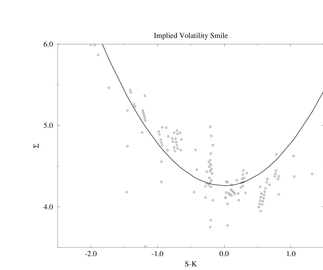
In a Black-Scholes universe, the implied volatility would in fact be a constant equal to the true volatility of the underlying asset. The non-dependence of implied volatility on the strike price can be viewed as a specification test for the Black-Scholes model. However, empirical studies of implied volatilities show a systematic dependence of implied volatilities on the exercise price and on maturity [Dumas (1996), Jackwerth (1996)]. In many cases the implied volatility presents a minimum at-the-money (when ) and has a convex, parabolic shape called the “smile” [Jackwerth (1996), Potters, Cont & Bouchaud (1998)] an example of which is given in figure 1. This is not always the case however: the implied volatility plotted as a function of the strike price may take various forms. Some of these alternative patterns, well known to options traders, are documented in [Dumas (1996)]. On many markets, the convex parabolic “smile” pattern observed frequently after the 1987 crash has been replaced in the recent years by a still convex but monotonically decreasing profile.
3.2 Implied distributions
The empirical evidence alluded to above points out to the misspecification of the Black-Scholes model and call for a satisfying explanation. If the SPD is not a lognormal then there is no reason that a single parameter, the implied volatility, should adequately summarize the information content of option prices. On the other hand, the availability of large data sets of option prices from organized markets such as the CBOE (Chicago Board of Options Exchange) add a complementary dimension to the data sets available for empirical research in finance: whereas time series data give one observation per date, options prices contain a whole cross section of prices for each maturity date and thus enable comparison between cross sectional and time series information, giving a richer view of market variables.
In theory, the information content of option prices is fully reflected by the knowledge of the entire density : this has led to developments of methods which, starting from a set of option prices search for a density such that Eq.(10) holds. Such a distribution is called an implied distribution, by analogy with implied volatility555Note that except when is a lognormal, the variance of the implied distribution does not coincide with the Black-Scholes implied volatility . If one adheres to the assumption of absence of arbitrage opportunities, the notion of implied distribution coincides with the concept of state price density defined above. But even if one does not adopt this point of view, the implied distribution still contains important information on the market. In the following we will use indifferently the terms “implied distribution” and “state price density” for . Let us now describe various methods for extracting information about the state price density from option prices.
4 Estimating state price densities
Given that all options prices can be expressed in terms of a single function, the state price density , one can imagine statistical procedures to extract from a sufficiently large set of option prices. Different methods have been proposed to reach this objective, among which we distinguish three different approaches. Expansion methods use a series expansion of the SPD which is then truncated to give a parametric approximation, the parameters of which can be calibrated to observed option prices. Non parametric methods do not make any specific assumption on the form of the SPD but require a lot of data. Parametric methods postulate a particular form for the SPD and fit the parameters to observed option prices.
4.1 Expansion methods
We regroup in this section various methods which have in common the use of a series expansion for the state price density. The general methodology can be stated as follows. One starts with an expansion formula for the state price density considered as a general probability distribution:
| (12) |
the first term of the expansion corresponding either to the lognormal or the normal distribution. The following terms can be therefore considered as successive corrections to the lognormal or normal approximations. The series is then truncated at a finite order, which gives a parametric approximation to the SPD which, if analytically tractable, enables explicit expressions to be obtained for prices of options. These expressions are then used to estimate the parameters of the model from market prices for options. Resubstituting in the expansion enables to retrieve an approximate expression for the SPD.
A general feature of these methods is that even when the infinite sum in the expansion represents a probability distribution, finite order approximations of it may become negative which leads to negative probabilities far enough in the tails. This drawback should not be viewed as prohibitive however: it only means that these methods should not be used to price options too far from the money.
We will review here three expansion methods: lognormal Edgeworth expansions [Jarrow & Rudd (1982)], cumulant expansions [Potters, Cont & Bouchaud (1998)] and Hermite polynomials [Abken et al. (1996)].
Cumulants and Edgeworth expansions
All these methods are based on a series expansion of the Fourier transform of a probability distribution (here, the state price density) defined by:
| (13) |
The cumulants of the probability density are then defined as the coefficients of the Taylor expansion:
| (14) |
The cumulants are related to the central moments by the relations
One can normalize the cumulants to obtain dimensionless quantities:
| (15) |
is called the skewness of the distribution , the kurtosis. The skewness is a measure of asymmetry of the distribution: for a distribution symmetric around its mean , while indicates more weight on the right side of the distribution. The kurtosis measures the fatness of the tails: for a normal distribution, a positive value of indicated a slowly decaying tail while distributions with a compact support often have negative kurtosis. A distribution with is said to be leptokurtic. An Edgeworth expansion is an expansion of the difference between two probability densities and in terms of their cumulants:
| (16) | |||||
Lognormal Edgeworth expansions
Since the density of reference used for evaluating payoffs in the Black-Scholes model is the lognormal density, Jarrow & Rudd [Jarrow & Rudd (1982)] suggested the use of the expansion above, taking as the state price density and as the lognormal density. The price of a call option, expressed by Eq. 10, is given by:
| (17) | |||||
where is the Black-Scholes price, the implied variance of the SPD and and are respectively the skewness and the kurtosis of the SPD and of the lognormal distribution. Given a set of option prices for maturity , Eq. 17 can then be used to determine the implied variance and the implied cumulants and .
This method has been applied by Corrado & Su [Corrado & Su (1996)] to S&P options: they extract the implied cumulants and for various maturities from option prices and show evidence of significant kurtosis and skewness in the implied distribution. Using the representation above, they propose to correct the Black-Scholes pricing formula for skewness and kurtosis by adding the first two terms in Eq.17. No comparison is made however between implied and historical parameters (cumulants of ).
Cumulant expansions and smile generators
Another method, proposed by Potters, Cont & Bouchaud [Potters, Cont & Bouchaud (1998)], is based on an expansion of the state price density starting from a normal distribution.
| (18) |
The first two terms are given by
| (19) | |||||
| (20) |
where is the skewness and the kurtosis of the density . Although the mathematical starting point here is quite similar to the Hermite or Edgeworth expansion, the procedure used by Potters et al is very different: instead of directly matching the parameters to option prices, they focus on reproducing correctly the shape of the volatility smile. Their procedure is the following: starting from the expansion (18) an analytic expression for the option price can be obtained in the form of series expansion containing the cumulants. The series is then truncated at a finite order and the expression for the option price inverted to give an analytical approximation for the volatility smile in terms of the cumulants up to order , expression as a polynomial of degree in . This expression is then fitted to the observed volatility smile (for example using a least squares method) to yield the implied cumulants.
An advantage of this formulation is that it corresponds more closely to market habits: indeed, option traders do not work with prices but with implied volatilities which they rightly considered to be more stable in time than option prices.
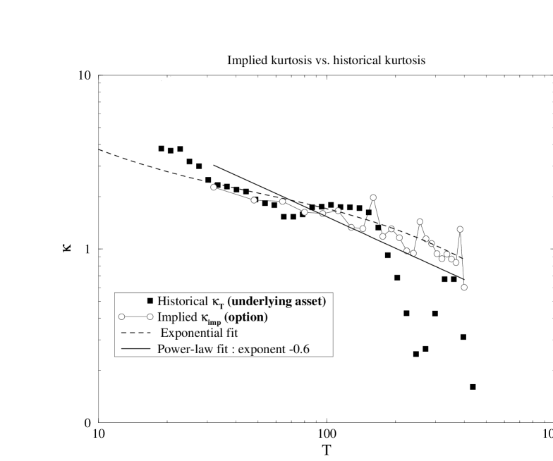
This analysis can be repeated for different maturities to yield the implied cumulants as a function of maturity : the resulting term structure of the cumulants then (shown in Fig.2) gives an insight into the evolution of the state price density under time-aggregation. By applying this method to options on BUND contracts on the LIFFE market, the authors show that the term structure of the implied kurtosis matches closely that of the historical kurtosis, at least for short maturities for which kurtosis effects are very important. This observation shows that the densities and have similar time-aggregation properties (dependence on ) a fact which is not easily explained in the arbitrage pricing framework where the relation between and is unknown in incomplete markets.
Although the expansion given in [Potters, Cont & Bouchaud (1998)] uses only the skewness and kurtosis, one could in principle move further in the expansion and use higher cumulants, which would lead to a polynomial expression for the implied volatility smile. However empirical estimates of higher order cumulants are unreliable because of their high standard deviations.
Hermite polynomial expansions
The -th Hermite polynomial is defined as:
| (21) |
The method recently proposed by Abken et al [Abken et al. (1996)] uses a Hermite polynomial expansion for both and the payoff function . Although the starting point is similar to the approach of [Potters, Cont & Bouchaud (1998)], the method is different: it is based on the properties of Hermite polynomials which form an orthonormal basis for the scalar product:
| (22) |
The state price density can be expanded on this basis:
| (23) |
Madan & Milne also use a representation of the payoff function in the Hermite polynomial basis:
| (24) |
Therefore, in contrast with the cumulant expansion method, not only the SPD is approximated but also the payoff. The coefficients can be calculated analytically for a given payoff function . In the case of a European call the coefficients are given in [Abken et al. (1996)]. The price of an option with payoff is then given by:
| (25) |
The price of any option can therefore be expressed as a linear combination of the coefficients , which correspond to the market price of “Hermite polynomial risk”. In order to retrieve these coefficients from option prices, one can truncate the expansion in Eq.25 at a certain order and, knowing the coefficients , calculate so as to reproduce as closely as possible a set of option prices, for example using a least-squares method. The state price density can then be reconstructed using Eq. 23. An empirical example is given in [Abken et al. (1996)] with : the empirical results show that both the historical and state price densities have significant kurtosis; however, the tails of the state price density are found to be fatter than those of the historical density, especially the left tail: the interpretation is that the market fears large negative jumps in the price that have not (yet!) been observed in the recent price history. Such results have also been reported in several other studies of option prices [Bates (1991), Ait-Sahalia et al. (1997)].
4.2 Non-parametric methods
One of the drawbacks of the Black-Scholes model is that it is based on a strong assumption for the form of the distribution of the underlying assets fluctuations, namely their lognormality. Although everybody agrees on the weaknesses of the lognormal model, it is not an easy task to propose a stochastic process reproducing in a satisfying manner the dynamics of asset prices [Cont (1998)].
Non-parametric methods enable to avoid this problem by using model-free statistical methods based on very few assumptions about the process generating the data. Two types of non-parametric methods have been proposed in the context of the study of option prices: kernel regression and maximum entropy techniques.
Kernel estimators
Ait Sahalia & Lo [Ait-Sahalia & Lo (1995)] have introduced another method based on the following observation by Breeden & Litzenberger [Breeden & Litzenberger (1978)]: if denotes the price of call option then the state price density can be obtained by taking the second derivative of with respect to the exercise price :
| (26) |
If one observed a sufficient range of exercise prices then Eq. 26 could be used in discrete form to estimate . However it is well known that the discrete derivative of an empirically estimated curve need not necessarily yield a good estimator of the theoretical derivative, let alone the second-order derivative. Ait-Sahalia & Lo propose to avoid this difficulty by using non-parametric kernel regression [Härdle (1990)]: kernel methods yield a smooth estimator of the function and under certain regularity conditions it can be shown that the second derivative of the estimator converges to for large samples. However the convergence is slowed down both because of differentiation and because of the “curse of dimensionality” i.e. the large number of parameters in the function .
Applying this method to S&P futures options, Ait-Sahalia & Lo obtain an estimator of the state price density for various maturities varying between 21 days and 9 months. The densities obtained are systematically different from a lognormal density and present significant skewness and kurtosis. But the interesting feature of this approach is that it yields the entire distribution and not only the moments or cumulants. One can then plot the SPD and compare it with the historical density or with various analytical distributions. Another important feature is that the method used by Ait-Sahalia & Lo also estimated the dependence on the maturity of the option prices, yielding, as in the cumulant expansion method, the term-structure (scaling behavior) of various statistical parameters as a by-product. However it is numerically intensive and difficult to use in real-time applications.
Maximum entropy method
The non-parametric methods described above minimize the distance between observed option prices and theoretical option prices obtained from a certain state price density . However such a problem has in principle an infinite number of solutions since the density has an infinite number of degrees of freedom constrained by a finite number of option prices. Indeed, different non-parametric procedures will not lead in general to the same estimated densities. This leads to the need for a criterion to choose between the numerous densities reproducing correctly the observed prices.
Two recent papers [Buchen & Kelly (1996), Stutzer (1996)] have proposed a method for estimating the state price density based on a statistical mechanics/ information theoretic approach, namely the maximum entropy method. The entropy of a probability density is defined as:
| (27) |
is a measure of the information content The idea is to choose, between all densities which price correctly an observed set of options, the one which has the maximum entropy i.e. maximizes under the constraint:
| (28) |
and subject to the constraint that a certain set of observed option prices are correctly reproduced:
| (29) |
This approach is interesting in several aspects. First, it is based on the minimization of an information criterion which seems less arbitrary than other penalty functions such as those used in other non-parametric methods. Second, one can generalize this method to minimize the Kullback-Leibler distance between and the historical density , defined as:
| (30) |
Minimizing this distance gives the state price density which is the “closest” to the historical density in an information-theoretic sense. This density should be related to the minimal martingale measure proposed by [Föllmer & Schweizer (1990)]. The value of can then give a straightforward answer to the question [Potters, Cont & Bouchaud (1998)]: how different is the SPD from the historical distribution? Or: how different are market prices of options from those obtained by naive expectation pricing (see section 2.2)?
However the absence of smoothness constraints has its drawbacks. One of the characteristics of this method is that it typically gives “bumpy” i.e. multimodal estimates of the state price density. This is due to the fact that, contrarily to the there is no constraint on the smoothness of the density. This may seem a bit strange because it is not the type of feature one expects to observe: for example, the historical PDFs of stock returns are always unimodal. This has to contrasted with the high degree of smoothness required in kernel regression methods. Some authors have argued that these bumps may be “intrinsic properties” of market data and should not be dismissed as aberrations but no economic explanation has been proposed. Jackwerth & Rubinstein [Jackwerth & Rubinstein (1996)] solve this problem by imposing smoothness constraints on the density: this can be done by subtracting from the optimization criterion a term penalizing large variations in the derivative . However the relative weight of smoothness vs.entropy terms may modify the results.
4.3 Parametric methods
Implied binomial trees
Apart from the Black-Scholes model, the other widely used option pricing model is the discrete-time binomial tree model [Cox & Rubinstein (1985)]. In the same way that continuous-time models can be used to extract continuous state price densities from market prices of options, the binomial tree model can be used to extract from option prices an “implied tree” the parameters of which are conditioned to reproduce correctly a set of observed option prices. Rubinstein [Rubinstein (1994)] proposes an algorithm which, starting from a set of option prices at a given maturity, constructs an implied binomial tree which reproduces them exactly. The implied tree contains the same type of information as the state price density presented above. The tree can then be used to price other options. Although discrete by definition, binomial trees can approximate as closely as one wishes any continuous state price density provided the number of nodes is large enough.
Rubinstein’s approach is easier to implement from a practical point of view than kernel methods and can perfectly fit a given set of option prices for any single maturity. However the large number of parameters may be a drawback when it comes to parameter stability: in practice the nodes of the binomial tree have to be recalculated every day and, as in the case of the Black-Scholes implied volatility, the implied transition probabilities will in general change with time.
Mixtures of lognormals
The habit of working with the lognormal distribution by reference to the Black-Scholes model has led to parametric models representing the state price density as a mixture of lognormals of different variances:
| (31) |
where is a lognormal distribution with unit variance and mean , the (risk-free) interest rate. The advantage of such a procedure is that the price of an option is simply obtained as the average of Black-Scholes prices for the different volatilities weighted by the respective weights of each distribution in the mixture. In principle one could interpret such a mixture as the outcome of a switching procedure between regimes of different volatility, the conditional SPD being lognormal in each case. Such models have been fitted to options prices in various markets by [Melick & Thomas (1992)].
Their results are not surprising: by construction, a mixture of lognormals has thin tails unless one allows high values of variance. But the major drawback of such a parametric form is probably its absence of theoretical or economic justification. Remember that the density which is modeled as a mixture of lognormals is not the historical density but the state price density: even in the hypothesis of market completeness it is not clear what sort of stochastic process for the underlying asset would give rise to such a state price density.
Method
Advantage
Disadvantage
Mixture of lognormals
Link with Black-Scholes
Too thin tails
Expansion methods
Easy to implement and interpret
Negative tails
Maximum entropy
Link with historical probability
Multimodality
Kernel methods
Gives the entire distribution
Slow convergence
Implied trees
Perfect fit of cross-sectional data
Parameter instability
5 Applications
5.1 Measuring investors’ preferences
If one considers a simple exchange economy [Lucas (1978)] with a representative investor then from the knowledge of any two of the three following ingredients it is theoretically possible to deduce the third one:
-
1.
The preferences of the representative investor.
-
2.
The stochastic process of the underlying asset.
-
3.
The prices of derivative assets.
Therefore, at least in theory, knowing the prices of a sufficient number of options and using time series data to obtain information about the price process of the underlying asset one can draw conclusions about the characteristics of the representative agents preferences. Such an approach has been proposed by Jackwerth [Jackwerth (1996)] to extract the degree of risk aversion of investors implied by option prices.
Exciting as it may seem, such an approach is limited as it stands for several reasons. First, while a representative investor approach may be justified in a normative context (which is the one adopted implicitly in option pricing theory) it does not make sense in a positive approach to the study of market prices. The limits of the concept of a representative agent have been already pointed out by many authors. Taking seriously the idea of a representative investor would imply all sorts of paradoxes, the absence of trade not being the least of them. Furthermore, even if the representative agent model were qualitatively correct, in order to obtain quantitative information on their preferences one must choose a parametric representation for the decision criterion adopted by the representative investor. Typically, this amounts to postulating that the representative investor maximizes the expectation of a certain utility function of her wealth ; depending on the choice for the form of the function one may obtain different results from the procedure described above. Given that utility functions are not empirically observable objects, the choice of a parametric family for is often ad-hoc thus reducing the interest of such an approach from an empirical point of view.
5.2 Pricing illiquid options
All options traded on a given underlying asset do not have the same liquidity: there are typically a few strikes and maturities for which the market activity is intense and the further one moves away from the money and towards longer maturities the less liquid the options become. It is therefore reasonable to consider that some options prices are more “accurate” than others in the sense their prices are more carefully arbitraged. These considerations must be taken into account when choosing the data to base the estimations on; for further discussion of this issue see [Ait-Sahalia & Lo (1995)].
Given this fact, one can then use the information contained in the market prices of liquid options -considered to be priced more “efficiently”- to price less liquid options in a coherent, arbitrage-free fashion. The idea is simple: first, the state price density is estimated by one of the methods explained above based only on market prices of liquid options; the estimated SPD is then used to calculate values of other, less liquid options. This method may be used for example to interpolate between existing maturities or exercice prices.
5.3 Arbitrage strategies
If one has an efficient method for pricing illiquid options ’better’ than the market then such a method can potentially be used for obtaining profits by systematically buying underpriced options and selling overpriced ones. These strategies are not arbitrage strategies in a textbook sense i.e. riskless strategies with positive payoff but they are statistical arbitrage strategies: they are supposed to give consistently positive returns in the long run.
The first such test was conducted by [Chiras & Manaster (1978)] who used the implied volatility as a predictor of future price volatility of the underlying asset. More recently Ait-Sahalia et al [Ait-Sahalia et al. (1997)] have proposed an arbitrage strategy based on non-parametric kernel estimators of the SPD. The idea is the following: one starts with a diffusion model for the stock price:
| (32) |
where the instantaneous volatility is considered to be a deterministic function of the price level . The function is then estimated from the historical price series of the underlying assets using a non-parametric approach. Under the assumption of a complete market, the state price density may be calculated from , yielding an estimator . Another estimator may be obtained by a kernel method as explained above. If options were priced according to the theory based on the assumption in Eq.32 then one would observe , a hypothesis which is rejected by the data. The authors then propose to exploit the difference between the two distributions to implement a simple trading strategy, which boils down to buying options for which the theoretical price calculated with is lower than the market price (given by ) and selling in the opposite case. They show that their strategy yields a steady profit ( annualized with a Sharpe ratio around 1.0) when tested on historical data. Such results have yet to be confirmed on other markets and data sets and it should be noted that large data sets are needed to implement them.
6 Discussion
We have described different methods for extracting the statistical information contained in market prices of options. There are several points which, in our opinion, should be kept in mind when using the results of such methods either in a theoretical context or in applications:
-
1.
All methods point out to the existence of fat tails, excess kurtosis and skewness in the state price density and clearly show that the state price density is different from a lognormal, as assumed in the Black-Scholes model. The Black-Scholes formula is simply used as a tool for translating prices into implied volatilities and not as a pricing method.
-
2.
The study of the evolution of the state price density under time aggregation shows a nontrivial term structure of the implied cumulants, resembling the terms structure of the historical cumulants. For example the term structure of the implied kurtosis shows a slow decrease with maturity which bears a striking similarity with that of historical kurtosis [Potters, Cont & Bouchaud (1998)]. In the terms used in the mathematical finance literature, the “risk-neutral” dynamics is not well described by a random walk / (geometric) Brownian motion model.
-
3.
One should not confuse the state price densities estimated by the approaches discussed above with the historical densities obtained from the historical evolution of the underlying asset. This confusion can be seen in many of the articles cited above: it amounts to implicitly assuming an expectation pricing rule. The two densities reflect two different types of information: while the historical densities reflects the fluctuations in the market price of the underlying asset, option prices and therefore the state price density reflects the anticipations and preferences of market participants rather than the actual (past or future) evolution of prices. This distinction is clearly emphasized in [Abken et al. (1996)] and more explicitly in the maximum entropy method [Stutzer (1996)] where even by minimizing the distance of the SPD with the historical distribution one finds two different distributions. Another way of stating this result is that option prices are not simply given by historical averages of their payoffs.
-
4.
More specifically, accessing the state price density empirically enables a direct comparison with the historical density which provides a tool for studying a central question in option pricing theory: the relation between the historical and the so-called “risk-neutral” density. The results show that the two distributions not only differ in their mean but may also differ in higher moments such as skewness or kurtosis.
In particular the “intuition” conveyed by the Black-Scholes model that the pricing density is simply a centered (zero-mean) version of the historical density is not correct. In this sense one sees that the Black-Scholes model is a “singularity” and its properties should not be considered as generic.
-
5.
Although this is implicitly assumed by many authors, it is not obvious that the state price densities estimated from options data do actually correspond to the “risk-neutral probabilities” or “martingale measures” [Harrison & Kreps (1979), Musiela & Rutkowski (1997)] used in the mathematical finance literature. Although constraint of the absence of arbitrage opportunities theoretically imposes that all option prices be expressed as expectations of their payoff with respect to the same density, the introduction of transaction costs and other market imperfections (limited liquidity for example) can allow for the simultaneous existence of several SPDs compatible with the observed prices. Indeed the presence of market imperfections may drastically modify the conclusions of arbitrage-based pricing theories [Figlewski (1989)]. In statistical terms, it is not clear whether a set of option prices determine the SPD uniquely in the presence of market imperfections even from a theoretical point of view (e.g. if one could observe an infinite number of strikes ). This issue has yet to be investigated both from a theoretical and empirical point of view.
The methods described above are becoming increasingly common in applications and will lead to an enhancement of arbitrage activities between the spot and option markets. Given the rapid development of options markets, the volume of such arbitrage trades is not negligible compared to the initial volume of the spot market, giving rise to non-negligible feedback effects. The existence of feedback implies that derivative asset such as call options cannot be priced in a framework where the underlying asset is considered as a totally exogenous stochastic process: the distinction between underlying and derivative asset becomes less clear-cut than what text-book definitions tend to make us think. The development of such “integrated” approaches to asset pricing should certainly be on the agenda of future research.
I would like to thank Yacine Ait-Sahalia, Jean-Pierre Aguilar, Jean-Philippe Bouchaud, Nicole El Karoui, Jeff Miller and Marc Potters for helpful discussions, Science & Finance SA for their hospitality and the organizers of the Budapest workshop, Janos Kertesz and Imre Kondor, for their invitation. The figures are taken from [Potters, Cont & Bouchaud (1998)].
References
- Abken et al. (1996) Abken P., Madan D.B. & Ramamurtie, S. (1996) ”Estimation of risk-neutral and statistical densities by Hermite polynomial approximation” Federal Reserve Bank of Atlanta.
- Ait-Sahalia & Lo (1995) Ait-Sahalia, Y. & Lo, A.H. (1996) ”Nonparametric estimation of state price dens ities implicit in financial asset prices ” NBER Working Paper 5351.
- Ait-Sahalia et al. (1997) Ait-Sahalia Y., Wang Y. & Yared, F. (1997) “Do option markets correctly assess the probabilities of movement of the underlying asset?”, Communication presented at Aarhus University Center for Analytical Finance, Sept. 1997.
- Bates (1991) Bates, D.S. (1995) “Post-87 crash fears in S&P 500 futures options” Wharton School Working Paper .
- Baxter & Rennie (1996) Baxter, M. & Rennie, A. (1996) Financial calculus , Cambridge University Press.
- Black & Scholes (1973) Black, F. & Scholes, M. (1973) ”The pricing of options and corporate liabiliti es” Journal of Political Economy, 81, 635-654.
- Bouchaud et al. (1995) Bouchaud, J.P., Iori, G. & Sornette, D. “Real world options: smile and residual risk” RISK, 1995.
- Bouchaud & Potters (1997) Bouchaud, J.P. & Potters, M. (1997) Théorie des Risques Financiers, Paris: Aléa Saclay.
- Breeden & Litzenberger (1978) Breeden, D. & Litzenberger, R. (1978) ”Prices of state-contingent claims implicit in options prices” Journal of Business, 51, 621-651.
- Buchen & Kelly (1996) Buchen, P.W. & Kelly, M. (1996) ”The maximum entropy distribution of an asset inferred from option prices” Journal of Financial & Quantitative Analysis, 31, 143-159.
- Chiras & Manaster (1978) Chiras, Donald P. & Manaster, Steven (1978) ”The information content of option prices and a test of market efficiency” Journal of Financial Economics, 6 187-211.
- Cont (1998) Cont, R. (1998) Statistical finance: empirical study and theoretical modeling of price variation in financial markets, PhD dissertation, Université de Paris XI.
- Corrado & Su (1996) Corrado, Charles J. & Su, Tie (1996) “Skewness and kurtosis in S&P500 index returns implied by option prices ” Journal of Financial Research XIX, No. 2, 175-192.
- Cox & Rubinstein (1985) Cox, J. & Rubinstein, M. (1985) Option markets, Prentice Hall.
- Debreu (1959) Debreu, G. (1959) The theory of value John Wiley & Sons, New York.
- Duffie (1992) Duffie, D. (1992) Dynamic asset pricing theory, Princeton University Press.
- Dumas (1996) Dumas B., Fleming J. & Whaley R.E. (1996) ”Implied volatility functions: empirical tests” HEC Working Paper.
- Eberlein & Jacod (1997) Eberlein, E. & Jacod, J. (1997) “On the range of options prices” Finance & Stochastics, 1 (2), 131-140.
- El Karoui & Quenez (1991) El Karoui, N. & M.C. Quenez (1991) ”Dynamic programming and pricing of contingent claims in incomplete markets” SIAM Journal of Control and Optimization.
- Figlewski (1989) Figlewski, S. (1989) “Options arbitrage in imperfect markets” Journal of Finance, XLIV (5), 1289-1311.
- Föllmer & Schweizer (1990) Föllmer, H. & Schweizer, M. (1990) “Hedging of contingent claims under incomplete information” in Davis, M.H.A & Elliott, R.J. (eds.) Applied Stochastic Analysis, Stochastic Monographs 5, London: Gordon & Breach, pp 389-414.
- Föllmer & Sondermann (1986) Föllmer, H. & Sondermann, D. (1986) ”Hedging of non redundant contingent claims ” Hildenbrand , W. & Mas-Colell, A. (eds.), Contributions to Mathematical Economics in Honor of Gérard Debreu, 205-223, North Holland, Amsterdam.
- Härdle (1990) Härdle, Wolfgang (1990) Applied non parametric regression, Cambridge University Press.
- Harrison & Kreps (1979) Harrison, J.M. & Kreps, D. (1979) ”Martingales and arbitrage in multiperiod securities markets” Journal of Economic Theory, 20, 381-408.
- Harrison & Pliska (1981) Harrison, J.M. & S. Pliska (1981) ”Martingales and stochastic integrals in the theory of continuous trading” Stochastic Processes and their applications, 11, 215-260.
- Jackwerth & Rubinstein (1996) Jackwerth, C.J. & Rubinstein, M. (1996) “Recovering probability distributions from contemporaneous security prices” Journal of Finance, December.
- Jackwerth (1996) Jackwerth, C.J. (1996) “Recovering risk aversion from option prices and realized returns” UC Berkeley Haas School of Business Working Paper.
- Jarrow & Rudd (1982) Jarrow, R. & Rudd, A. (1982) ”Approximate option valuation for arbitrary stochastic processes” in Journal of Financial Economics 10, 347-369.
- Lucas (1978) Lucas, R.E. (1978) “Asset prices in an exchange economy” Econometrica, 46, 1429-1446.
- Melick & Thomas (1992) Melick, W.R. & Thomas, C.P. (1997) “Recovering an assets implied PDF from options prices: an application to crude oil during the Gulf crisis” Journal of Financial and Quantitative Analysis, 32, 91-116.
- Merton (1992) Merton, Robert C. (1992) Continuous-time finance, Blackwell Publishers.
- Musiela & Rutkowski (1997) Musiela, M. & Rutkowski, M. (1997) Martingale methods in financial modeling, Berlin: Springer.
- Potters, Cont & Bouchaud (1998) Potters M., Cont R. & Bouchaud, J.P. (1998) “Financial markets as adaptive systems” Europhysics Letters, 41 (3).
- Rubinstein (1994) Rubinstein, M. (1994) “Implied binomial trees” Journal of Finance, 49, 771-818.
- Ruelle (1987) Ruelle, D. (1987) Chaotic dynamics and strange attractors Cambridge: Cambridge University Press.
- Schäl (1994) Schäl, M. (1994) ”On quadratic cost criteria for option hedging”, Mathematics of operations research,19, 121-131.
- Schmalensee & Trippi (1978) Schmalensee, R. & Trippi, R.R. (1978) ”Common stock volatility expectations implied by option prices” Journal of Finance, 33, 129-147.
- Shimko (1993) Shimko, D. (1993) “Bounds of probability” RISK, 6 (4), 33-37.
- Stutzer (1996) Stutzer, M. (1996) “A simple nonparametric approach to derivative security valuation” Journal of Finance, 101, (5), 1633-1652.