[

Synchronization of Short-Range Pulse-Coupled Oscillators

Abstract

We explore systems of pulse-coupled oscillators beyond the mean-field limit [R.E. Mirollo and S.H. Strogatz, SIAM J. Appl. Math. 50, 1645 (1990)] by means of a manageable description which leads to a great simplification of the dynamics. Sufficient conditions for synchronization are exactly obtained for a ring with nearest-neighbor directed interactions, turning out to be the same as in the all-to-all case. Our analysis shows new synchronization mechanisms occurring when the interactions are local.

]

Nonequilibrium spatially extended dynamical systems, consisting of many degrees of freedom, constitute one of the most frequent manifestations in nature, which however still require new approaches to be understood [2]. Very remarkable in them is the spontaneous emergence of order, i.e., self-organization, by means of local, short-range interactions that cooperate to build correlations over all spatial and temporal scales [3]. Among all forms of order in space and time, synchronization and periodicity are the strongest ones, respectively, and play a crucial role in many physical, chemical, and biological systems [4, 5, 6].

Systems behaving in this way are in fact populations of oscillators coupled between them; in particular, outstanding examples make it clear that in most living systems the interaction between units cannot be viewed as continuous in time but rather as discontinuous and episodic, in the form of sharp pulses from one oscillator to another. Pacemaker cells in the heart [7], neurons in the visual cortex [8], and fireflies that flash on and off simultaneously in periodic intermittency [9] provide striking illustrations of spontaneous synchronous evolution in nature, all of them with pulsatile interactions.

The discontinuous character of the coupling makes remarkably difficult the mathematical analysis of these systems. In the case of a network of all-to-all pulse-coupled oscillators, Mirollo and Strogatz, however, were able to overcome the hardness of the problem establishing a sufficient condition for synchronization [10]. Their result is based on the idea of absorption, which means that once two oscillators get synchronized they never desynchronize. In this way, they proved that, no matter the initial conditions, synchronization arises cooperatively by a sequence of absorptions, in a self-organized process where no cell leads the population but it is the whole that coordinates the overall activity to achieve self-synchronization.

In contrast to the Mirollo and Strogatz’s scenario and other situations with all-to-all, or mean-field, interactions [11, 12, 13, 14], for more realistic networks [15], in which the firing of one unit does not modify the state of all the others in the same way, the concept of absorption is no longer valid and the synchrony achieved by a subset of oscillators can be lost [16, 17]. Thereby, in these cases one would expect a weaker tendency to synchronize, as occurs in other large networks of oscillators. Numerical studies [18], however, indicate that the conditions for synchronization in networks with reduced connectivity seem to be the same as in the all-to-all case. Despite this counterintuitive result was already conjectured by Mirollo and Strogatz [10], up to now there is no proof of synchronization in any model of pulse-coupled oscillators beyond the mean-field assumption.

In this Letter we address precisely the problem of establishing sufficient conditions for synchronization to occur in networks of pulse-coupled oscillators with local connectivity. In this regard, we have exactly derived them for the Mirollo and Strogatz’s model with nearest-neighbor directed coupling in one dimension, turning out to be the same as in the mean-field case [10]. This kind of feed-forward connectivities arise frequently in the modeling of some layered structures of the brain [19], whereas in loop-like circuits, they are relevant for cardiac arrhythmia and the brain clock [20].

Consider a population of $N$ relaxation or integrate-and-fire oscillators, where the units evolve in time integrating an excitatory driving signal until the state variable of some of them reaches a threshold, firing an instantaneous zero-width pulse to their neighbors, and then relaxing to a lower-value state, where the driving acts again. In general, any system of oscillators can be described in terms of the phases $\phi_{i}$ of its units [14, 21]. For relaxation oscillators $\phi_{i}$ measures the normalized elapsed time since the last firing of unit $i$ if there had been no interactions. The time evolution of the units is then given by

$$\mbox{if }\phi_{i}<1\ \forall i\Rightarrow\frac{d\phi_{i}}{dt}=\frac{1}{T},\ \ i=1,2,\dots N,\ \ \ \ \hskip 50.00008pt$$ (1)

(2)

$$\mbox{if }\phi_{i}\geq 1\Rightarrow\left\{\begin{array}[]{lll}\phi_{i}&\rightarrow&0,\\ \phi_{n(i)}&\rightarrow&\phi_{n(i)}+\Delta(\phi_{n(i)})\ \ \mbox{ if }\phi_{n(i)}>0,\end{array}\right.$$ (5)

where $T$ is the period of the oscillators and $\Delta(\phi)$ the so-called phase response curve, which gives the phase shift of a unit when it gets a pulse from a neighbor. Neighbors of unit $i$ are denoted by $n(i)$ and for a one-dimensional directed lattice with coupling “from left to right”, $n(i)=i+1$. Periodic boundary conditions are taken assuming $N+1\equiv 1$ and $0\equiv N$.

Notice that $T$ and $\Delta(\phi)$ are the same for all the units, which therefore are identical and identically coupled. Observe also that a unit at the reset point, $\phi=0$, does not feel the incoming pulse; this is a way to include the effects of absolute refractoriness. In addition, as in the Mirollo-Strogatz model, we only deal with excitatory interactions, i.e., $\Delta(\phi)>0,\forall\phi$; this makes the interaction process evolve in the form of avalanches.

We will show that a sufficient condition for complete synchronization is obtained when the phase response curve is an increasing function of the phase, i.e., $\Delta^{\prime}(\phi)>0,\forall\phi$. Our proof of synchrony consists of two differentiated parts. The first one establishes that once an oscillator has fired triggered by the firing of its neighbor, both units will fire at the same time forever, even though they may lose their mutual synchrony between firings. We call such a process a capture. The second part shows how for almost all initial conditions there is a capture for each pair of neighboring units. In this way, as eventually every pair of neighbors are mutually captured, the firing of one unit will ensure the firing of the rest and the complete synchrony of the whole population will be achieved, with all the units evolving with the same phase.

In order to prove our first claim, let us consider two neighboring units, labeled by $i$ and $i+1$, which have fired at the same time. Since both units have the same free time evolution, they can only desynchronize when the $i$th one gets a pulse; when this happens, at time $a$, its phase $\phi^{a-}_{i}$ is instantaneously increased by an amount $\Delta(\phi^{a-}_{i})$. Here the superscript of the phase indicates time. Notice that just before the pulse both phases are equal, i.e.,

$$\phi^{a-}_{i}=\phi^{a-}_{i+1}\;.$$ (6)

In contrast, just after the pulse the phase of the $(i+1)$th unit remains at the same value, in principle, whereas the phase of the $i$th unit changes to

$$\phi^{a+}_{i}=\phi^{a-}_{i}+\Delta(\phi^{a-}_{i})\;.$$ (7)

At this point, two different situations may occur depending on whether the $i$th unit crosses the threshold as a consequence of the received pulse or not.

If $\phi^{a-}_{i}+\Delta(\phi^{a-}_{i})>1$ the unit crosses the threshold and fires, increasing then the phase of its right neighbor by an amount $\Delta(\phi^{a-}_{i+1})$. Since $\Delta(\phi^{a-}_{i+1})=\Delta(\phi^{a-}_{i})$, the $(i+1)$th unit also crosses the threshold, firing at the same time as the $i$th one.

If $\phi^{a-}_{i}+\Delta(\phi^{a-}_{i})<1$ the $i$th unit does not reach the threshold. Therefore, after receiving the pulse its phase increases continuously in time until either it reaches the threshold or it gets another pulse. In the former case, the unit fires at time $b=a+T[1-\phi^{a-}_{i}-\Delta(\phi^{a-}_{i})]$, sending a pulse of strength $\Delta(\phi^{b-}_{i+1})$ to $i+1$. Notice that as

$$\phi^{b-}_{i+1}=1-\Delta(\phi^{a-}_{i})\;,$$ (8)

the phase of $i+1$ after the pulse will be

$$\phi^{b+}_{i+1}=1-\Delta(\phi^{a-}_{i})+\Delta(\phi^{b-}_{i+1})\;.$$ (9)

Assuming that $\Delta(\phi)$ is an increasing function of its argument, $\phi^{b+}_{i+1}$ is greater than $1$. Consequently the $(i+1)$th unit crosses the threshold, firing then at the same time as its left neighbor.

Let us now discuss the case in which the $i$th unit receives two pulses. Indeed, as the strength of the pulses is not fixed, a unit can overtake its right neighbor; this is what makes a unit get more than one pulse while its phase is evolving between $0$ and $1$. For the sake of generality we also consider that a set of connected units on the left of $i$ also get two pulses, except the leftmost unit of this set, denoted by $L$, which only gets a single pulse. The existence of a unit receiving only a single pulse is guaranteed by the periodic conditions and by the fact that at least $i+2$ gets only one pulse before $i+1$ can reach the threshold. After sending the first pulse to unit $j$, $j-1$ is delayed with respect to $j$ and consequently

$$\phi^{a_{j-1}}_{j-1}<\phi^{a_{j-1}}_{j}\;,\;\;\forall j\mbox{~{}~{}s.t.~{}~{}}L<j\leq i\;,$$ (10)

where the superscript ${a_{j-1}}$ indicates any time between the first firing of the $(j-1)$th unit and the time in which $j-1$ gets its first pulse in this cycle. In order for a unit $j$ to get the second pulse, the second firing of its left neighbor must occur before the second firing of $j$. The sequence of firings of this set is then from left to right, starting on the $L$th unit. Therefore, just before and after the $L$th unit gets its only pulse at time $a$, its phase must be smaller and greater, respectively, than the corresponding ones of the remaining units in the group, i.e.,

$$\phi^{a-}_{L}<\phi^{a-}_{j}<\phi^{a-}_{L}+\Delta(\phi^{a-}_{L})\;,\;\;\forall j\mbox{~{}~{}s.t.~{}~{}}L<j\leq i+1\;.$$ (11)

Once the $L$th unit reaches the threshold at time $b=a+T[1-\phi^{a-}_{L}-\Delta(\phi^{a-}_{L})]$, all units from $L$ to $i+1$ fire because

$$\phi^{b+}_{j}=1+\phi^{a-}_{j}-\phi^{a-}_{L}+\Delta[\phi^{b-}_{j}]-\Delta[\phi^{a-}_{L}]>1\;,$$ (12)

$$\;\;\forall j\mbox{~{}~{}s.t.~{}~{}}L<j\leq i+1\;,$$ (13)

since $\Delta^{\prime}(\phi)>0$, $\forall\phi$ and $\phi^{b-}_{j}>\phi^{a-}_{L}\;,\;\;\forall j\mbox{~{}~{}s.t.~{}~{}}L<j\leq i+1$.

Our analysis then indicates that once two neighboring units fire at the same time, they always remain firing at the same time if the left unit only gets one or two pulses. The case in which the left unit gets three or more consecutive pulses is not allowed in this process because a unit reaches the threshold and fires when it gets the second pulse, as we have shown.

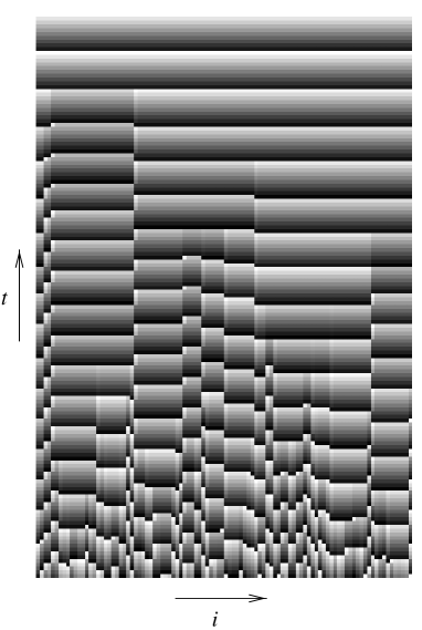
FIG. 1.: Spatiotemporal evolution of a ring of 100 oscillators for $\Delta(\phi)=\varepsilon+\gamma\phi$, with $\varepsilon=0.01$ and $\gamma=0.3$. Black and white colors stand for minimum and maximum values of the phase $\phi_{i}$, respectively. Notice that the coupling is “from left to right”.

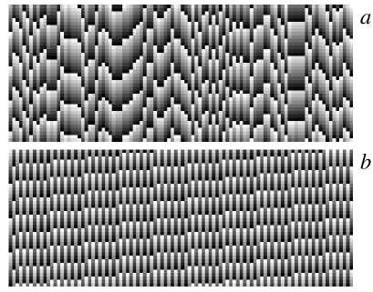
FIG. 2.: (a) Same situation as in Fig. 1 but $\varepsilon=0.1$ and $\gamma=0$. (b) Same situation as in Fig. 1 but $\varepsilon=0.7$ and $\gamma=-0.1$.

Concerning our second statement, we now demonstrate that the set ${\cal A}^{0}$ of initial conditions of an arbitrary oscillator for which it will never fire at the same time as its left neighbor has Lebesgue measure zero. To be precise, for a unit $i+1$ and given an initial configuration of the rest of the population, the set ${\cal A}^{0}_{i+1}$ is defined as

$${\cal A}^{0}_{i+1}\equiv{\bf\{}\phi^{0}_{i+1}\mbox{ s.t. $i$ will not capture $i+1$ and}$$ (14)

$$i i+1$$ will not be captured in an avalanche triggered by , (15)

provided that the rest of the population (16)

$$\mbox{is in an initial state $\{\phi_{j}^{0}\}_{j\neq i+1}$ }{\bf\}}.$$ (17)

In particular, if $\phi^{0}_{i}=1$, ${\cal A}^{0}_{i+1}\subset\{\phi^{0}_{i+1}$ s.t. $0<\phi^{0}_{i+1}<1-\Delta(\phi^{\star})\}$, where $\phi^{\star}$ is defined by $\phi^{\star}+\Delta(\phi^{\star})\equiv 1$; otherwise, $i$ captures $i+1$ immediately. In essence, the proof shows that for almost all the initial conditions of a unit, and irrespective of the state of the rest, it cannot be confined forever in the interval $(0,1-\Delta(\phi^{\star}))$ receiving an infinite number of pulses from its neighbor.

Due to the characteristics of the dynamics, the time evolution of any unit can be decomposed into two parts. On the one hand, the free time evolution in which the unit does not get any pulse is given by

$$\phi(t^{\prime})\equiv F^{t^{\prime}-t}[\phi(t)]=\left(\phi(t)+{t^{\prime}-t\over T}\right)\;\mbox{mod}\;1\;,$$ (18)

where $t$ and $t^{\prime}$ are times between two consecutive pulses. Notice that time is now indicated by the argument of the phase. On the other hand, the dynamics of the unit is coupled to its neighbors. Thereby, when its left neighbor fires the unit gets a pulse and increases its phase by an amount $\Delta(\phi)$, provided that it is neither brought to the threshold nor refractory, which, by definition, is always fulfilled for the time evolution of the set ${\cal A}^{0}$. Then, the new phase just after the firing is

$$\phi^{n+1}(t)\equiv h[\phi^{n}(t)]=\phi^{n}(t)+\Delta[\phi^{n}(t)]\;,$$ (19)

with the superscript $n$ indicating now the number of pulses received by the unit.

It can be seen that the measure $\mu$ of the time evolution of the set ${\cal A}^{0}$ remains invariant during the free time evolution by using that

$${dF^{t^{\prime}-t}(\phi)\over d\phi}=1\ \ \mbox{for}\ 0\leq\phi<1\;.$$ (20)

Indeed, if ${\cal A}(t^{\prime})$ denotes the state of the set ${\cal A}^{0}$ after a time $t^{\prime}$,

$$\mu[{\cal A}(t^{\prime})]=\int_{{\cal A}(t^{\prime})}d\mu[\phi(t^{\prime})]=\int_{{\cal A}(t)}{dF^{t^{\prime}-t}[\phi(t)]\over d\phi(t)}d\mu[\phi(t)]$$ (21)

$$=\int_{{\cal A}(t)}d\mu[\phi(t)]=\mu[{\cal A}(t)]\;.$$ (22)

In contrast, when the unit gets a pulse, the measure evolves in such a way that the inequality

$$\mu({\cal A}^{n+1})\geq\left(1+\tilde{\Delta^{\prime}}\right)\mu({\cal A}^{n})$$ (23)

holds, with $\tilde{\Delta^{\prime}}\equiv\min[\Delta^{\prime}(\phi)]$ and ${\cal A}^{n+1}$ being the resulting of the evolution of the set ${\cal A}^{0}$ after the $n+1$ pulses. This follows directly from both

$$\mu({\cal A}^{n+1})=\int_{{\cal A}^{n+1}}d\mu(\phi^{n+1})=\int_{{\cal A}^{n}}{dh(\phi^{n})\over d\phi^{n}}d\mu(\phi^{n})$$ (24)

and $dh(\phi^{n})/d\phi^{n}=1+\Delta^{\prime}(\phi^{n})\geq 1+\tilde{\Delta^{\prime}}$. If $\Delta(\phi)$ is an increasing function of its argument, its derivative is positive and then $1+\tilde{\Delta^{\prime}}$ is greater than 1. In consequence, if the unit always gets the pulse at $\phi\in(0,1-\Delta(\phi^{\star}))$, when $n$ goes to infinity the inequality

$$\mu({\cal A}^{0})\leq{\mu({\cal A}^{n+1})\over(1+\tilde{\Delta^{\prime}})^{n+1}}$$ (25)

implies that the set ${\cal A}^{0}$ has zero measure since $\mu({\cal A}^{n+1})$ is bounded by $1-\Delta(\phi^{\star})$.

In other words, the flow in phase space remains incompressible during the driving; however, if $\Delta^{\prime}(\phi)>0$, $\forall\phi$, the coupling acts in a more complicated way, expanding the volume elements with each firing, except in the case of a capture, where the volume contracts. This is the process which eventually dominates, leading the population to the complete-synchronization attractor. In addition, it is easy to show that this condition is fully equivalent to the one obtained by Mirollo and Strogatz [21].

To illustrate the essentials of the emergence of synchrony in systems with explicit spatial dependence, in Fig. 1 we have depicted the results obtained from numerical simulations for a directed ring when the condition $\Delta^{\prime}(\phi)>0$, $\forall\phi$, is satisfied. This figure shows the time evolution towards the synchronized attractor, starting from a random initial condition. It is evidenced how the complete synchrony of the whole population is achieved through a coarsening process in which the domains of captured oscillators grow until eventually all the units are evolving with the same phase. In contrast, in Fig. 2 we show the time evolution for two situations wherein synchronization does not appear. Fig. 2a corresponds to a case in which $\Delta^{\prime}(\phi)=0$, $\forall\phi$. In this situation, starting from a random initial condition, perpetual disorganization occurs; the system remains evolving periodically in time in a spatially disordered state. The situation shown in Fig. 2b corresponds to a typical pattern reached after a long transient (not displayed) for $\Delta^{\prime}(\phi)<0$, $\forall\phi$. In this case, synchronization does not occur although the final pattern looks more regular than that of Fig. 2a.

In summary, we have established, for the first time, sufficient conditions for synchronization in a general model of pulse-coupled oscillators with local interactions, ensuring that, on a directed ring, they are the same as in the mean field case. The simple model of rhythmic oscillations in biological systems we have presented illustrates the fundamentals of emergence of organization in nonequilibrium complex systems led by local rules, in contrast to previous work devoted only to global coupling. Our analysis, then, elucidates new mechanisms taking place to attain synchrony when the spatial structure is explicitly considered [22].

We enjoyed very much the discussions with Steven Strogatz during the XV Sitges Conference, whose organization is also acknowleged by A.C. for providing financial support to attend it. J.M.G.V.’s work is financed by a grant of the CIRIT and DGICYT’s research program No. PB95-0881.

REFERENCES

- [1] E-mail addresses: vilar@ffn.ub.es, corral@nbi.dk.
- [2] S.H. Strogatz, Nature (London) 378, 444 (1995).
- [3] P. Bak, How Nature Works (Copernicus, Springer-Verlag, New York, 1996).
- [4] A.T. Winfree, The Geometry of Biological Time (Springer-Verlag, New York, 1980).
- [5] Y. Kuramoto, Chemical Oscillations, Waves, and Turbulence (Springer-Verlag, Berlin, 1984).
- [6] S.H. Strogatz, in Frontiers in Mathematical Biology, edited by S.A. Levin, Lecture Notes in Biomathematics, Vol. 100, 122 (Springer-Verlag, Berlin, 1994); K. Wiesenfeld et al., Phys. Rev. Lett. 76, 404 (1996).
- [7] C.S. Peskin, Mathematical Aspects of Heart Physiology, (Courant Institute of Mathematical Sciences, New York University, New York, 1975), p. 268.
- [8] C.M. Gray et al., Nature (London) 338, 334 (1989).
- [9] J. Buck and E. Buck, Sci. Am. 234, 74 (1974).
- [10] R.E. Mirollo and S.H. Strogatz, SIAM J. Appl. Math. 50, 1645 (1990).
- [11] Y. Kuramoto, Physica D 50, 15 (1991); C.-C. Chen, Phys. Rev. E 49, 2668 (1994); S. Bottani, Phys. Rev. Lett. 74, 4189 (1995); Phys. Rev. E 54, 2334 (1996).
- [12] L.F. Abbott and C. van Vreeswijk, Phys. Rev. E 48, 1483 (1993); A. Treves, Network 4, 259 (1993); M. Tsodyks et al., Phys. Rev. Lett. 71, 1280 (1993).
- [13] C. van Vreeswijk et al., J. Comp. Neur. 1, 313 (1994); U. Ernst et al., Phys. Rev. Lett. 74, 1570 (1995).
- [14] W. Gerstner, Phys. Rev. E 51, 738 (1995).
- [15] D.J. Watts and S.H. Strogatz, Nature (London) 393, 440 (1998).
- [16] A. Corral et al., Phys. Rev. Lett. 74, 118 (1995); A. Corral et al., Phys. Rev. Lett. 78, 1492 (1997).
- [17] P.C. Bressloff et al., Phys. Rev. Lett. 79, 2791 (1997); P.C. Bressloff and S. Coombes, Phys. Rev. Lett. 80, 4815 (1998).
- [18] A. Corral et al., Phys. Rev. Lett. 75, 3697 (1995).
- [19] J. Hertz, A. Krogh, and R.G. Palmer, Introduction to the Theory of Neural Computation (Addison-Wesley, Redwood, 1991).
- [20] H. Ito and L. Glass, Physica D 56, 84 (1991); J. McCrone, New Scientist No. 2106, 52 (1997).
- [21] A. Díaz-Guilera et al., Physica D 103, 419 (1997).
- [22] I. Stewart, Nature (London) 350, 557 (1991).