[

Comment on “Symmetry properties of magnetization in
the Hubbard model at finite temperature”

Abstract

The results of G. Su and M. Suzuki [Phys. Rev. B 54, 8291 (1996); ibidem 57, 13367 (1998)] for the spin and pseudo-spin symmetry properties of the Hubbard model are reexamined. We point out that the exact relations they have found are valid down to zero temperature and that their solutions for both spin and pseudo-spin correlation functions are incorrect.

]

In a recent paper G. Su and M. Suzuki[2] analyze the spin symmetry properties enjoyed by the Hubbard model in presence of an homogeneous external magnetic field. They derive at finite temperatures an exact relation connecting the spin correlation function to the magnetization. Also, the authors claim to have found without any a priori assumption at least one of the exact solutions for the magnetization as function of the applied field. This result follows previous works[3, 4] for the pseudo-spin counterpart where a solution for the pseudo-spin correlation as a function of the filling has been assessed.

In this Comment we clarify the issue of applicability of the exact relations, by use of the equation of motion, showing that they are valid also at zero temperature. Furthermore, we show that the pretended solutions for both spin and pseudo-spin correlation functions are incorrect.

The Hubbard model in presence of an homogeneous external magnetic field $h$ reads as

$$H = \sum_{ij}\left(t_{ij}-\mu\delta_{ij}\right)c^{\dagger}(i)c(j)+U\sum_{i}n_{\uparrow}(i)n_{\downarrow}(i)$$ (1)

$$- h\sum_{i}s_{z}(i)$$ (2)

where $s_{z}(i)$ is the third component of the spin density operator.

Let us introduce the total spin operators

$$S^{+} = \sum_{i}c^{\dagger}_{\uparrow}(i)c_{\downarrow}(i)$$ (3)

$$S^{-} = \sum_{i}c^{\dagger}_{\downarrow}(i)c_{\uparrow}(i)$$ (4)

$$S_{z} = \frac{1}{2}\sum_{i}\left(c^{\dagger}_{\uparrow}(i)c_{\uparrow}(i)-c^{\dagger}_{\downarrow}(i)c_{\downarrow}(i)\right)$$ (5)

and the thermal retarded Green’s function

$$S^{+-}\left(t-t^{\prime}\right) = \left\langle{\cal R}\left[S^{+}(t)S^{-}\left(t^{\prime}\right)\right]\right\rangle$$ (6)

$$= \frac{i}{2\pi}\int_{-\infty}^{+\infty}\!\!\!\!\!\!d\omega\,e^{-i\omega\left(t-t^{\prime}\right)}S^{+-}(\omega)$$ (7)

By means of the Hamiltonian (2) the spin operators satisfy the Heisenberg equations

$$i\frac{\partial}{\partial t}S^{\pm}=\pm 2hS^{\pm}\;\;\;\;\;\;\;\;\;\;i\frac{\partial}{\partial t}S^{z}=0$$ (8)

Then, we have

$$\frac{1}{N}S^{+-}(\omega)=\frac{2m}{\omega-2h+i\eta}$$ (9)

where $N$ is the number of sites and $m$ is the magnetization per site

$$m=\frac{1}{N}\left\langle S_{z}\right\rangle$$ (10)

In presence of an external magnetic field the spin symmetry is explicitly broken, [cfr. Eq. (8)], and the propagator $S^{+-}(\omega)$ exhibits a massive collective mode[5] $\omega=2h$. When $h=0$ and $m\neq 0$ the collective mode becomes gapless, in accordance with the Goldstone theorem.

From Eq. (9), by standard methods, we obtain the spin correlation function

$$\frac{1}{N}\left\langle S^{+}\left(t\right)S^{-}\left(t^{\prime}\right)\right\rangle=\frac{2m\,e^{-2ih\left(t-t^{\prime}\right)}}{1-e^{-2\beta h}}$$ (11)

where $\beta=1/\!k_{\mathrm{B}}T$. Similarly, we derive

$$\frac{1}{N}\left\langle S^{-}\left(t\right)S^{+}\left(t^{\prime}\right)\right\rangle=-\frac{2m\,e^{2ih\left(t-t^{\prime}\right)}}{1-e^{2\beta h}}$$ (12)

Let us note that (11) and (12) satisfy the KMS relation:

$$\left\langle S^{+}\left(t\right)S^{-}\left(t^{\prime}+i\beta\right)\right\rangle=\left\langle S^{-}\left(t^{\prime}\right)S^{+}\left(t\right)\right\rangle$$ (13)

In the static case Eqs. (11) and (12) become

$$\frac{1}{N}\left\langle S^{+}S^{-}\right\rangle = m\left[\coth\left(\beta h\right)+1\right]$$ (14)

$$\frac{1}{N}\left\langle S^{-}S^{+}\right\rangle = m\left[\coth\left(\beta h\right)-1\right]$$ (15)

These are the exact relations derived by Su and Suzuki[2]; however they are not restricted at finite temperature, but hold also at $T=0$. In particular, for finite magnetic field

$$\lim_{T\rightarrow 0}\frac{1}{N}\left\langle S^{+}S^{-}\right\rangle = 2m$$ (16)

$$\lim_{T\rightarrow 0}\frac{1}{N}\left\langle S^{-}S^{+}\right\rangle = 0$$ (17)

On the basis of the relations (15) Su and Suzuki[2] promote as one of the exact solutions for the magnetization as a function of the applied magnetic field the following expression

$$m\left(h,T\right)=\frac{n}{2}\tanh\left(\beta h\right)$$ (18)

where $n$ is the particle density. Also, they stress that other solutions, if they exist, might have similar forms. At the opposite, the solution depicted in (18) is clearly wrong except for the limiting case of half-filling and infinite $U$. Indeed, the pretended solution (18) can be falsified by looking at two exactly solvable limits of the Hubbard model. That is, the noninteracting [i.e. $U=0$] and atomic [i.e. $t_{ij}=0$] ones.

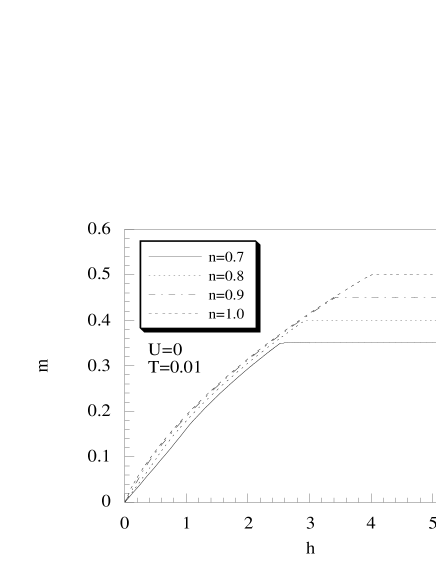
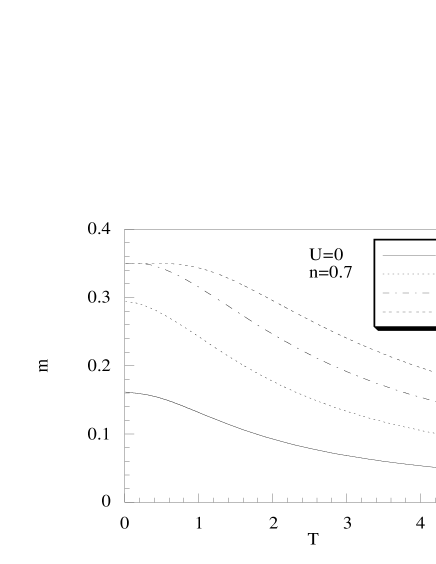
FIG. 1.: Magnetization $m$ as a function of filling $n$, applied magnetic field $h$ and temperature $T$.

Non interacting case

It is direct to see that

$$n = 1-\frac{\Omega}{2\left(2\pi\right)^{d}}\int_{\Omega_{\mathrm{B}}}\!\!\!d^{d}k\left[T_{\uparrow}({\bf k})+T_{\downarrow}({\bf k})\right]$$ (19)

$$m = \frac{1}{4}\tanh\left(\beta h\right)\left[1-\frac{\Omega}{\left(2\pi\right)^{d}}\int_{\Omega_{\mathrm{B}}}\!\!\!d^{d}k\,T_{\uparrow}({\bf k})T_{\downarrow}({\bf k})\right]$$ (20)

$\Omega$ is the volume of the unit cell, $d$ is the dimensionality of the system and $\Omega_{\mathrm{B}}$ is the first Brillouin zone. We put $T_{\sigma}({\bf k})=\tanh\left[\beta\,E_{\sigma}\right({\bf k})/2]$ with energy spectra

$$E_{\uparrow}({\bf k}) = -\mu-4t\alpha({\bf k})-h$$ (21)

$$E_{\downarrow}({\bf k}) = -\mu-4t\alpha({\bf k})+h$$ (22)

where $\alpha({\bf k})=1/\!d\sum_{i=1}^{d}\cos\left(k_{i}a\right)$, $t$ is the hopping integral and $a$ is the lattice constant.

In the two-dimensional case the magnetization is shown (cfr. Fig. 1) for different values of the parameters $n$, $T$ and $h$. The solution (18), proposed in Ref. [2], obviously is not a solution for the case $U=0$.

Atomic limit

In this case it is easy to show that

$$n = \frac{1-\frac{1}{2}\left(T_{1}+T_{3}\right)+\frac{1}{4}\left(1-T_{3}\right)\left(T_{1}-T_{2}\right)}{1-\frac{1}{4}\left(T_{1}-T_{2}\right)\left(T_{3}-T_{4}\right)}$$ (23)

$$+ \frac{\frac{1}{4}\left(1-T_{1}\right)\left(T_{3}-T_{4}\right)}{1-\frac{1}{4}\left(T_{1}-T_{2}\right)\left(T_{3}-T_{4}\right)}$$ (24)

$$2m = \frac{\frac{1}{2}\left(T_{3}-T_{1}\right)+\frac{1}{4}\left(1-T_{3}\right)\left(T_{1}-T_{2}\right)}{1-\frac{1}{4}\left(T_{1}-T_{2}\right)\left(T_{3}-T_{4}\right)}$$ (25)

$$- \frac{\frac{1}{4}\left(1-T_{1}\right)\left(T_{3}-T_{4}\right)}{1-\frac{1}{4}\left(T_{1}-T_{2}\right)\left(T_{3}-T_{4}\right)}$$ (26)

where $T_{i}=\tanh\left(\beta\,E_{i}/2\right)$ with energy spectra

$$E_{1} = -\mu-h$$ (27)

$$E_{2} = -\mu+U-h$$ (28)

$$E_{3} = -\mu+h$$ (29)

$$E_{4} = -\mu+U+h$$ (30)

We note that for $\mu=U/2$ the previous expressions become

$$n = 1$$ (31)

$$m = -\frac{T_{1}+T_{2}}{4\left[1+\frac{1}{2}\left(T_{1}-T_{2}\right)\right]}=\frac{T_{h}\left(1+T_{U}\right)}{2\left(1+T_{U}T^{2}_{h}\right)}$$ (32)

with

$$T_{U}=\tanh\left(\beta\,U/\!4\right)\;\;\;\;\;\;\;\;T_{h}=\tanh\left(\beta\,h/2\right)$$ (33)

In particular, in the limit of large $U$ and for finite temperature

$$m\rightarrow\frac{T_{h}}{1+T^{2}_{h}}=\frac{1}{2}\tanh\left(\beta\,h\right)$$ (34)

in agreement with the result of Ref. [6].

An intrinsic symmetry of the Hubbard model is the pseudo-spin $SU(2)$ symmetry[7] that combined with the spin $SU(2)$ one yields the $[SU(2)\otimes SU(2)]/\!Z_{2}=SO(4)$ symmetry group. The generators of this transformation are given by the total pseudo-spin operators

$$P^{+} = \sum_{i}e^{i{\bf Q}\cdot{\bf R}_{i}}c^{\dagger}_{\uparrow}(i)c^{\dagger}_{\downarrow}(i)$$ (35)

$$P^{-} = \sum_{i}e^{-i{\bf Q}\cdot{\bf R}_{i}}c_{\downarrow}(i)c_{\uparrow}(i)$$ (36)

$$P_{z} = \frac{1}{2}\sum_{i}\left[n(i)-1\right]$$ (37)

where ${\bf Q}=(\pi,\pi)$. These operators satisfy the Heisenberg equations

$$i\frac{\partial}{\partial t}P^{\pm}=\pm(2\mu-U)P^{\pm}\;\;\;\;\;\;\;\;\;\;i\frac{\partial}{\partial t}P_{z}=0$$ (38)

Let us consider the thermal retarded Green’s function

$$P^{+-}\left(t-t^{\prime}\right) = \left\langle{\cal R}\left[P^{+}(t)P^{-}\left(t^{\prime}\right)\right]\right\rangle$$ (39)

$$= \frac{i}{2\pi}\int_{-\infty}^{+\infty}\!\!\!\!\!\!d\omega\,e^{-i\omega\left(t-t^{\prime}\right)}P^{+-}(\omega)$$ (40)

By means of the equation of motion (38) we find

$$\frac{1}{N}P^{+-}(\omega)=\frac{n-1}{\omega-(2\mu-U)+i\eta}$$ (41)

The Hamiltonian has pseudo-spin $SU(2)$ symmetry only at half-filling; when $n\neq 1$ the symmetry is explicitly broken. Again, this is seen in the propagator where a massive collective mode $\omega=2\mu-U$ is observed[5]. From (41) we obtain the correlation function

$$\frac{1}{N}\left\langle P^{+}\left(t\right)P^{-}\left(t^{\prime}\right)\right\rangle=\frac{(n-1)\,e^{-i(2\mu-U)\left(t-t^{\prime}\right)}}{1-e^{-\beta(2\mu-U)}}$$ (42)

and similarly

$$\frac{1}{N}\left\langle P^{-}\left(t\right)P^{+}\left(t^{\prime}\right)\right\rangle=-\frac{(n-1)\,e^{i(2\mu-U)\left(t-t^{\prime}\right)}}{1-e^{\beta(2\mu-U)}}$$ (43)

It is easy to see that (42) and (43) satisfy the KMS relation. In the static case:

$$\frac{1}{N}\left\langle P^{+}P^{-}\right\rangle = \frac{1}{2}(n-1)\left[\coth\left(\beta(2\mu-U)/2\right)+1\right]$$ (44)

$$\frac{1}{N}\left\langle P^{-}P^{+}\right\rangle = \frac{1}{2}(n-1)\left[\coth\left(\beta(2\mu-U)/2\right)-1\right]$$ (45)

which give

$$\left\langle P^{+}P^{-}\right\rangle=e^{\beta(2\mu-U)}\left\langle P^{-}P^{+}\right\rangle$$ (46)

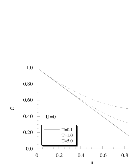
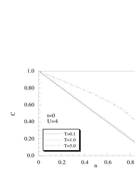
FIG. 2.: $C$ as a function of filling $n$, intrasite Coulomb repulsion $U$ and temperature $T$.

These exact results relates the pseudo-spin correlation functions to the particle number $n$ and are a manifestation of the intrinsic symmetry. These relations generalize at $T=0$ the results previously obtained by Su[4].

Under the particle-hole transformation we have the following relations

$$\mu(2-n)=U-\mu(n)\;\;\;\;\;\;\;\;C^{+-}(2-n)=C^{-+}(n)$$ (47)

where we put $C^{+-}=\left\langle P^{+}P^{-}\right\rangle$, $C^{-+}=\left\langle P^{-}P^{+}\right\rangle$. Use of Eq. (46) leads to

$$C^{+-}(2-n)=e^{-\beta\left[2\mu(n)-U\right]}C^{+-}(n)$$ (48)

By making use of the transformation properties (47), it is easy to see that the expression (45) satisfies the property (48). Actually, this is a manifestation of the intimate interrelation between pseudo-spin and particle-hole symmetries[8].

In Ref. [4] the particle-hole symmetry is tautologically used as a supplementary equation and the following solution for the pseudo-spin correlation function is presented for the case $h=0$

$$\frac{1}{N}\left\langle P^{+}P^{-}\right\rangle=\frac{C(T)}{1+e^{-\beta(2\mu-U)}}$$ (49)

where $C(T)$ is an unknown function of temperature only. When (49) is used in (45) one is lead to the following equation for the chemical potential

$$n=1+C(T)\tanh\left[\beta(\mu-U2)\right]$$ (50)

This equation is incorrect. For example, let us consider the limit of small temperature. Then, (50) would give $n\rightarrow 1-C(0)$, which is clearly wrong.

In Fig. 2 we present the function $C(n,T,U)=(n-1)\coth\left[\beta(\mu-U2)\right]$ as a function of $n$ for various temperatures, in the non-interacting and atomic limits. It is clear that $C$ is not a function of temperature only, as stated in Ref. [4], but varies with $n$ and $U$.

In conclusion, we have shown that the symmetry properties (15) and (45), obtained in Refs. [2, 3, 4], can be derived by means of the equation of motion and are valid for any temperature, including also zero temperature. These relations are exact relations and are valid for any dimension of the system; for any value of the Hubbard interaction $U$ and of the applied magnetic field $h$. Furthermore, they relate bosonic and fermionic propagators. Indeed, any approximation method should satisfy them in order to treat on equal footing one- and two- particle Green’s functions, and to preserve spin and pseudo-spin symmetries[9]. We have also shown that the solutions proposed in Refs. [2] and [4] for the magnetization and for the particle density are not valid.

REFERENCES

[1] Present address: Serin Physics Laboratory, Rutgers University,
Piscataway, New Jersey 08854, USA.
[2] G. Su and M. Suzuki, Phys. Rev. B 57, 13367 (1998).
[3] G. Su, Phys. Letters A 220, 263 (1996).
[4] G. Su, Phys. Rev. B 54, 8281 (1996).
[5] S.-Q. Shen and X. C. Xie, Condensed Matter 8, 4805
(1996).
[6] A. Süto, Phys. Rev. B 43, 8779 (1991).
[7] C. N. Yang, Phys. Rev. Lett. 62, 2144 (1989).
[8] H. Bruus and J.-C. Anglés d’Auriac, Phys. Rev. B 55, 9142 (1997).
[9] F. Mancini and A. Avella, cond-mat/9807019, Condensed Matter
Physics (in print).