Theory of Boundary Effects in Invasion Percolation

Abstract

We study the boundary effects in invasion percolation with and without trapping. We find that the presence of boundaries introduces a new set of surface critical exponents, as in the case of standard percolation. Numerical simulations show a fractal dimension, for the region of the percolating cluster near the boundary, remarkably different from the bulk one. In fact, on the surface we find a value of $D^{sur}=1.65\pm 0.02$ (for IP with trapping $D_{tr}^{sur}=1.59\pm 0.03$), compared with the bulk value of $D^{bul}=1.88\pm 0.02$ ($D_{tr}^{bul}=1.85\pm 0.02$). We find a logarithmic cross-over from surface to bulk fractal properties, as one would expect from the finite-size theory of critical systems. The distribution of the quenched variables on the growing interface near the boundary self–organises into an asymptotic shape characterized by a discontinuity at a value $x_{c}=0.5$, which coincides with the bulk critical threshold. The exponent $\tau^{sur}$ of the boundary avalanche distribution for IP without trapping is $\tau^{sur}=1.56\pm 0.05$; this value is very near to the bulk one. Then we conclude that only the geometrical properties (fractal dimension) of the model are affected by the presence of a boundary, while other statistical and dynamical properties are unchanged. Furthermore, we are able to present a theoretical computation of the relevant critical exponents near the boundary. This analysis combines two recently introduced theoretical tools, the Fixed Scale Transformation (FST) and the Run Time Statistics (RTS), which are particularly suited for the study of irreversible self–organised growth models with quenched disorder. Our theoretical results are in rather good agreement with numerical data.

]

I Introduction

Recently, a large effort has been devoted to the study of Invasion Percolation (IP)[1, 2, 3]. Compared to standard percolation [4], IP has the advantage of describing the dynamical evolution of the invading cluster as well as the final result. Furthermore, since a connectivity condition is naturally implemented in IP, its dynamics do not produce extra, undesired, finite clusters, as happens instead in standard percolation [4]. Even if IP is more difficult to treat theoretically (because it presents a non-local, extremal deterministic dynamics in a quenched disordered medium [2, 5]), it has been considered the paradigm of a large class of self–organised critical models . The Bak and Sneppen model for punctuated equilibrium [6], and the Sneppen model for surface dynamics [7] belong to this class.

In the standard theory of critical phenomena, the role of boundaries has been intensively analysed [8], and for many physical situations, ranging from Ising models to the more recent class of Self Organized Models [9, 10], their presence produces a novel set of critical indices related to the surface. The reason for the new behaviour consists in the lack of a microscopic layer in the system. This changes dramatically the microscopic interactions in the surface region of the system, yielding eventually to a macroscopically observable characteristic behaviour. The standard theory of finite size scaling of a thermodynamical system close to its critical point predicts in two dimensions [11] a logarithmic cross-over of the critical exponents from the boundary to the bulk. Consequently, the effect of the boundary extends over the whole system. This is due to the strong correlations peculiar to a critical system. Such a study has already been done for standard percolation, and the results are available in the literature [12, 13], but no similar analysis has been performed for IP. Among the approaches applied to models with extremal dynamics, going from Mean Field treatment [5] to a recently introduced technique called Run Time Statistics [2, 14], only the latter one, when combined with the Fixed Scale Transformation method [15], seems to be able to capture the subtle effects due to the presence of a boundary in the system.

In this work we present numerical and theoretical evidence that a peculiar behaviour on the boundary takes place also in IP. Some of the results reported have already been published [16]. Here, we would like to give a complete and detailed description of numerical results and of the derivation of the analytical results of the previous Ref.[16]. Moreover, we present new analytical and numerical results, like the computation of the boundary avalanche exponent and the extension of our analysis to the case of IP with trapping, which has no analogue in the standard percolation model. In particular, the results for IP with trapping have no counterpart in standard percolation theory [4].

From a qualitative point of view, the analogy between boundary effects in ordinary critical phenomena and IP can be easily understood by considering that boundary sites have fewer neighbors than bulk ones and hence fewer chances to invade a new region. Moreover, IP is a self–organised critical model and, as the evolution time tends to infinity, it can be considered in the same way as an ordinary thermodynamical system when the temperature is tuned at the critical value $T_{c}$. The crossover between boundary and bulk fractal properties is shown by considering intersections of the percolation cluster with straight lines parallel to the external boundary. This subset of the percolating cluster has a fractal dimension that varies with the distance from the boundary. Using some theoretical tools introduced for the study of fractal growth processes, the Run Time Statistics (RTS) [2, 14] and the Fixed Scale Transformation (FST) [15], we are able to study analytically this behaviour, with an estimation of the boundary fractal dimension that is in rather good agreement with the numerical value. This is done for IP with and without trapping. In addition we study the avalanche dynamics near the boundary, for IP without trapping, and we compute both numerically and analytically, by using the RTS and FST schemes, the boundary avalanche exponent $\tau^{sur}$.

Our results are presented in the following order. In section II, we present the definition of the model and a review of the numerical data. In section III, we describe the concepts underlying RTS and FST. In section IV we apply these methods to the computation of the boundary fractal dimension. In section V we compute the boundary avalanche exponent. In the last part we give a summary of the main topics.Appendix A is devoted to the derivation of the RTS equations.

II The Invasion Percolation Model

IP was introduced more than 10 years ago [1] in order to describe the slow capillary displacement of a fluid (e.g. oil), the defender, from a random porous medium due to another immiscible invading fluid (e.g. water), the invader.

In general two cases are studied: 1) the medium is filled with an incompressible defender (e.g. oil), which is immiscible with the invader fluid; 2) the medium is filled with a defender with an infinite compressibility. In the former case the invader may trap regions of the defender: e.g. as the water advances, it can completely surround regions of the oil. These regions become disconnected from the other bonds occupied by the defender and, due to incompressibility, they become forbidden to the invader. This trapping effect lowers the fractal dimension of the percolating invader cluster. From an experimental point of view, trapping is connected to the phenomenon of “residual oil”, which is a great economic problem in the oil industry [17].

The random medium is represented by a network of bonds corresponding to the throats connecting the pores of the medium. Let us assume, now, that the invader begins to displace the defender. Under the condition of a low and constant flow rate, the interface can be considered to move one step at time, by invading the throat with the smallest section, i.e. the throat where there is the largest capillary force [1]. One can mimic this behaviour by assigning a random section $x_{i}$ (here we take an uniform distribution in $\left[0,1\right]$) to each bond $i$ of the medium. The invading cluster evolves by occupying the bond with the smallest $x_{i}$ on its perimeter. This is what is called a deterministic extremal dynamics.

To study the behaviour at the boundary of this model, we performed some numerical simulations in the system shown in FIG.1, representing a sample of a two dimensional square lattice. To study the effect of only one boundary (e.g. the left one), we ensured isolation from the other one. To obtain this, we choose a lattice with size $HL\times 2L$ where $H=2,3,4$, and the initial invader cluster is composed of the first L bonds of the bottom line, starting from the left boundary. The simulation stops when the cluster percolates the system, i.e. when the growth reaches the top of the sample.

In FIG.2 a typical realization of this process is shown. The region of interest is the bottom-left one in FIG.1, where we can assume that the region is “frozen” with respect to the invasion process, i.e. the asymptotic fractal properties of the percolating cluster are well defined. For each value of the system size $L$ we collected a set of $10^{3}$ different realizations. In the region where statistics is collected, we study the fractal dimension of the sets of points obtained by intersecting the percolating cluster with lines parallel to the boundary, at a distance $z$ from it. In this way, we are able to follow the cross-over of the fractal dimension of the cluster from the boundary to the bulk region. A standard box-counting procedure is used to compute the fractal dimension of the intersections. The behaviour of the fractal dimension $d(z/L)$ of the intersections as a function of the normalized distance $z/L$ from the left boundary is presented in FIG.3 for $L=256,H=4$ (i.e. $512\times 1024$). In Table I we present the values of the boundary fractal dimension $d^{sur}$ for different system sizes $L$ and different values of $H$. For the largest simulation $L=256$, $H=4$ (i.e. $512\times 1024$), we obtain the result that the fractal dimension of this subset of the cluster passes from $d^{sur}=0.65\pm 0.02$ on the boundary to $d^{bul}=0.88\pm 0.02$ in the bulk (at a distance $z/L\sim 0.4$ from the boundary), where $d^{bul}$ represents the fractal dimension of the intersection far away from the boundary. A similar behaviour holds for smaller sizes $L$ and $H$ as well. Since the dimension of the intersection set $d$ obeys $d=D-1$ where $D$ is the fractal dimension of the cluster, the last result is in agreement with the known value of $D\simeq 1.89$.

In order to explain such a slow crossover from $d^{sur}$ to $d^{bul}$ we assumed that the number of occupied sites $N(z,L)$ at a distance $z$ from the boundary follows the finite-size scaling law:

$$N(z,L)=L^{d^{bul}}f(z/L)$$ (1)

where one has $f(z/L)\sim(z/L)^{(d^{bul}-d^{sur})}$ for $z<<L$ and $f(z/L)=\em{const}$ for $z>>L$. Then in the first region we should have:

$$d(z)=d^{sur}+(d^{bul}-d^{sur})log(z)/log(L)$$ (2)

To test this scaling hypothesis we collapsed the curves relative to different $L$ by plotting $\left[d(z)-d^{sur}\right]log(L)$ as a function of $z$. The result depicted in FIG.4 shows a rather good collapse in the small $z$ region. A similar behaviour is found for IP with site trapping. In order to implement site trapping in our simulations, after each growth step a fictitious Laplacian field $\phi$ is relaxed on the growing structure, with the following boundary conditions: $\phi=0$ on the bottom boundary, the left boundary and the invading cluster, while $\phi=1$ on the top boundary. In this way, all the bonds in a closed, trapped region are characterized by $\phi=0$. Then it is possible to recognize trapped bonds and to eliminate them from the list of bonds allowed to grow at the next step. Obviously, in this case the numerical simulations need much more time to be performed and we have been able to collect a smaller, but still significative, statistics with respect to IP without trapping ($10^{3}$ clusters for $L=64$, $2\times 10^{2}$ clusters for $L=128$ and $10^{2}$ clusters for $L=256$ each one for $H=2,3,4$). In FIG. 5 we show the behaviour of the intersection dimension $d_{tr}(z/L)$ versus the normalized distance from the boundary, each simulation is for a values of $H=4$. The fractal dimension $d_{tr}$ is computed on samples $512\times 1024$ (i.e. $L=256$ and $H=4$) and passes from $d_{tr}^{sur}=0.59\pm 0.03$ on the boundary to $d_{tr}^{bul}=D_{tr}^{bul}-1=0.85\pm 0.03$ in the bulk, which is agreement with the known value $D_{f}\sim 1.82$ for site trapping [1]. The data shown in Table II exhibit the same slow logarithmic cross-over found for IP without trapping.

Other important quantities characterizing the dynamical properties of IP are the average distribution of quenched variables on the perimeter, called histogram $\Phi_{t}(x)$, which gives an evidence of the self–organised nature of the model, and the avalanche-size distribution in the asymptotic critical state $Q(s;x_{c})$, where $x_{c}$ is the ”self-critical” threshold of the model.

Let us start with the study of the histogram for IP without trapping. It is known[14] that for the bulk IP, the histogram distribution evolves in time from the initial flat shape, and self–organises into a step function with a discontinuity at a critical value $x_{c}^{bul}$ which depends on the details of the model and on the embedding dimension [1] and coincides with the critical threshold of the classical percolation in the same kind of lattice. For the two dimensional square lattice one has $x_{c}^{bul}=\frac{1}{2}$. Our simulations show that the distribution of the $x_{i}$’s on the boundary self–organises into a theta function and the critical threshold is again $x_{c}^{bul}$. A comparison between the bulk histogram and the boundary one is shown in FIG.6. It is not surprising to find a similar behaviour, because the value of the boundary critical threshold is dependent on the dynamical evolution of the whole percolating cluster. Since for bulk IP the trapping does not affect the histogram distribution [1], the introduction of the trapping does not modify the above result.

Another important quantity describing the dynamics of the model is the critical avalanche-size distribution $Q(s;x_{c})$. An avalanche is a sequence of elementary growths events causally and geometrically connected to a first one, which is called the initiator of the avalanche. That is, if one consider an event of growth of the initiator (a certain bond $k$), the avalanche lasts until the bonds selected to grow are those joining the growth interface after the growth of bond $k$ (bonds “younger” than $k$). Note that all these bonds have the related random number $x$ smaller than the initiator one. If the bond selected by the dynamics was on the perimeter before the initiator growth, then the avalanche stops. In the asymptotic limit, due to the step shape of the histogram, only bonds with $x\leq x_{c}$ grow. We call $Q(s;x)$ the size distribution of avalanches whose initiator is associated with a number equal to $x$. It is shown for bulk IP, both through numerical simulations and theoretical calculation, $Q(s;x)$ is scale invariant (i.e. is a power law), only if the variable $x$ of the initiator is equal to $x_{c}$. If $x<x_{c}$ $Q(s;x)$ has an exponential cut off at a typical size $s_{0}\sim(x_{c}-x)^{-\sigma}$ with $\sigma>0$. The avalanche distribution $Q(s;x_{c})$ for bulk IP without trapping has a power law shape with an exponent $\tau^{bul}\sim 1.60\pm 0.02$ [2, 18]. The dynamical activity near the boundary can be characterized by the distribution of the avalanches whose first bond (initiator) is located on the boundary. We performed a set of about $10^{3}$ numerical simulations of IP without trapping, of size $3L\times 5L$ with $L=128$, lasting $4\times 10^{5}$ time steps and collected the statistics of boundary avalanches from the last $2\times 10^{5}$ time steps, in order to ensure that the system is in its asymptotic critical state. To identify the single avalanche, we followed [2], by adding the condition that the initiator of the avalanche is on the boundary. In FIG.7 we show the behaviour of the boundary avalanche distribution. We find: $\tau^{sur}=1.56\pm 0.05$. This value is very near to the bulk value, and we can conclude from our numerical analysis that bulk and boundary avalanches have the same distribution. In section V we will derive analytically this result.

III Run Time Statistics and Fixed Scale Transformation

In this section we introduce the theoretical tools we used to compute the boundary fractal dimension $d^{sur}$ of the infinite IP cluster and the boundary avalanche exponent $\tau^{sur}$. Our strategy combines Fixed Scale Transformation (FST) [15] and Run Time Statistics (RTS) [2, 14]. We describe briefly the FST approach and we focus more on the RTS.

FST is a lattice path integral scheme allowing one to evaluate the spatial correlation properties of the intersection between an infinite fractal cluster and a straight line. This approach is based on the statistical invariance of the correlation properties under a parallel translation of the intersecting line (valid for fractals which are homogeneous, at least in the translation direction). In particular, it is possible to compute the probabilities $C_{0}$,$C_{1}$ and $C_{2}$ related to the configurations $0,1,2$ of the fine graining process of FIG.8. For the normalization condition it follows:

$$C_{0}+C_{1}+C_{2}=1$$ (3)

From these probabilities one can compute the fractal dimension of the intersection by:

$$d=\frac{log(C_{0}+C_{1}+2C_{2})}{log2}=\frac{log(1+C_{2})}{log2}$$ (4)

As usual, due to the intersection dimension rule, the fractal dimension $D$ of the analysed cluster is given by $D=1+d$. The probabilities $C_{0},C_{1}$ and $C_{2}$ are computed through the statistical weights of growth paths, once a stochastic dynamical formulation of the model is given. This means that the use of FST is straightforward whenever a simple calculation of the growth paths on the lattice is possible. In the present case, there are two problems to overcome in applying the FST.

Firstly, the fractal properties of the system depend on the distance from the boundary ($C_{0}=C_{0}(z),C_{1}=C_{1}(z),C_{2}=C_{2}(z)$), this extrapolation from the intersection dimension to the global dimension is no more allowed. Moreover, what we actually can compute with the FST method are the local (near to the boundary) correlations orthogonal to the boundary, while the fractal dimension of the intersection set parallel to the boundary is given by the correlation properties parallel to the boundary. However, since the crossover of the fractal dimension from the boundary to the bulk is very slow (logarithmic), one is allowed to assume that the cluster is ”locally” isotropic. In this case transversal and horizontal correlations in a thin (with respect to the system size) strip parallel to the boundary share similar properties. For the same reason, we can evaluate the fractal dimension $d$ of the intersection between the cluster and a straight line parallel to the lateral boundary, through the first neighbors correlations orthogonal to the same boundary at the same distance.

Secondly for IP (and for any other model with deterministic extremal dynamics) the calculation of the growth paths is extremely difficult, because the weight of a path cannot be written as the product of the probabilities of the single steps composing it. The extremal dynamics of IP is deterministic, and the disorder appears only as a realization of quenched random variables. This implies that to evaluate the statistical weight of a given path we have to perform an average over all the quenched disorder and this average does not factorize itself in the product of the averages of the single steps composing the path. The latter problem is solved by the introduction of the RTS transformation. This transformation allows us to represent a quenched-extremal process like a stochastic dynamics.

As regards the RTS (for a more detailed discussion see [2]), the starting point is, at each time step $t$, to consider an effective probability density $\rho_{i,t}(x)$ for the random number $x_{i}$ associated to each bond $i$ of the growing interface $\partial{\cal C}_{t}$. This density depends on the growth history of the dynamics. In fact, $\rho_{i,t}(x)dx$ gives the probability that the variable $x_{i}$ for the bond $i$ at time $t$ is in the interval $\left[x,x+dx\right]$, conditioned by the past growth dynamics of the cluster. If a bond $i$ does not belong to the cluster, or to the growth interface, its effective probability density is the flat one. Meanwhile, the bonds on the growth interface show a more interesting form of distribution. Once the densities $\rho_{i,t}(x)$ for each bond $i$ on the interface are known, one can calculate the growth probability distribution $\{\mu_{i,t}\}$ (i.e. the probability of being the minimum on the interface) at that time step for each interface bond (see appendix A):

$$\mu_{i,t}=\int_{0}^{1}dx\rho_{i,t}(x)\prod_{j\in\partial{\cal C}_{t}-\{i\}}\left[\int_{x}^{1}dy\rho_{j,t}(y)\right].$$ (5)

where $\partial{\cal C}_{t}-\{i\}$ represents the growth interface at time $t$ except for the bond $i$. The effective probability density of any surviving bond $j$ at time $t+1$ on the interface must then be updated, conditioned to the previous growth history at time $t$, i.e. the growth of the bond $i$. The corresponding equation is (see appendix A):

$$\rho_{j,t+1}(x)=\frac{\rho_{j,t}(x)}{\mu_{i,t}}\int_{0}^{x}dy\rho_{i,t}(y)\prod_{k\in\partial{\cal C}_{t}-\{i,j\}}\left[\int_{y}^{1}dz\rho_{k,t}(z)\right]$$ (6)

where $\partial{\cal C}_{t}-\{i,j\}$ is the growth interface except for bonds $i$ and $j$. New bonds added to the perimeter are assigned an effective probability density according to a uniform distribution in $\left[0,1\right]$, as no information is available about them till this time step.

The above formalism allows us to write the statistical weight of a path as the product of the probabilities of individual steps.

IV Computation of the boundary fractal dimension

In order to combine the FST and the RTS approach, we need to have scale invariant growth rules (we want to compute a critical exponent, the fractal dimension, and the result cannot depend on the scale). The extremal dynamics of IP is known to be independent on the choice of the initial distribution of quenched variables. By using this symmetry, one can show that the scale invariant dynamics for block variables is identical to the microscopic dynamics [2]. The FST performs the computation of the correlation properties of a given structure by considering only the growth processes inside a growth column (FIG. 9). This approximation has been shown to be a good one for the dielectric breakdown model (DBM) [19], and for bulk IP [2]. Since eqs. (5), (6) involve all the variables on the perimeter of the growing cluster, a limitation of the process in the growth column destroys these correlations, leading to compact clusters [2]. The solution to this problem is given by observing that, as the critical avalanche size distribution is a power law, the statistical properties of a generic one (i.e. an avalanche whose initiator $i$ has $x_{i}=x_{c}$) are then scale invariant. Then if one considers the dynamical evolution of a generic critical avalanche inside the growth column one obtains the scale invariant correlation properties (i.e. $C_{0}$, $C_{1}$ and $C_{2}$) needed to compute the fractal dimension. This can be done by modifying the eqs. (5), (6), in order to take account the dynamical evolution of a single critical avalanche. We consider a growth column on the perimeter of the infinite structure ($t\rightarrow\infty$). The starting point is the observation that scale invariant asymptotic avalanches begin with an initiator at $x=x_{c}$, due to the asymptotic shape of the histogram. All the memory of the past growth history is then contained in the requirement that the initiator has $x=x_{c}$. Then one is allowed to consider explicitly only the bonds grown after the growth of the initiator.

The RTS dynamics corresponding to the local scale invariant dynamics, is obtained by

• considering only bonds inside the growth column;

• imposing that any “active” bond $i$ in the column can grow only if the value of its variable $x_{i}$ is less than $x_{c}=1/2$. The idea is that if $x_{i}>x_{c}$ for all the bonds in the growth column, growth will occur at some other place in the structure outside the growth column (it coincides with the definition of scale invariant avalanche);

• imposing that the initial bond (i.e. the initiator), which is the largest of the variables participating to the growth process, has exactly $x_{i}=x_{c}$.

In this way we modified the Eqs. (5) and (6), limiting the product over the perimeter variables to variables inside the growth column.

Because of the presence of a lateral surface, this model is intrinsically anisotropic, and consequently we have to introduce some modification to the usual way of performing the FST for the bulk IP. The anisotropy of the environment implies a breaking of symmetry in the FST basic configurations in FIG.8. Then, due to the presence of the boundary, the probabilities $C_{0}$ and $C_{1}$ are not equal in this case.

Through the FST one may compute directly the matrix elements $M_{ij}$ and from the relation:

$$\left(\begin{array}[]{c}C_{0}\\ C_{1}\\ C_{2}\\ \end{array}\right)=\left(\begin{array}[]{ccc}M_{00}&M_{10}&M_{20}\\ M_{01}&M_{11}&M_{21}\\ M_{02}&M_{12}&M_{22}\\ \end{array}\right)\left(\begin{array}[]{c}C_{0}\\ C_{1}\\ C_{2}\\ \end{array}\right)$$ (7)

it is possible to evaluate $C_{2}$ and, by using Eq.(4), $d$. In this case

$$M_{01}=M_{10}=0$$ (8)

and

$$C_{2}=\frac{M_{12}M_{02}}{M_{12}+M_{21}(M_{02}-M_{12})+M_{12}(M_{02}-M_{22})}$$ (9)

The anisotropy of the environment is also introduced in the lateral boundary condition of the growth column where the FST calculation is performed. At the left side of the column we impose the presence of a rigid wall and at the right side the paths are allowed to go out and then to return inside the growth column, as can be seen in FIG.10. In this way we have obtained the results shown in Tab.III, where the fractal dimension for increasing order $n$ (the path length) of the FST computation is given. We used a power law fit (FIG.11) to extrapolate $d^{sur}(n)$ to $n=\infty$ and obtained $d^{sur}(\infty)\simeq 0.70$.

A similar approach has been applied to IP with site trapping, in particular: when a growth path produces a closed region surrounding the initial pair configuration $C_{i}$ (see FIG. 10), it stops and its statistical weight contributes to the matrix elements $M_{i,1}$, since the empty right (or left) site above the initial configuration cannot be occupied anymore. The results are shown in Tab.IV and in FIG.12. We have extrapolated our results to $n=\infty$ by using the following function (see FIG.12):

$$d_{tr}^{sur}(n)=\frac{1}{n}exp(-n^{\alpha})$$ (10)

with $\alpha=0.66$. This extrapolation gives $d_{tr}^{sur}(\infty)\simeq 0.66$.

V Computation of the boundary avalanche exponent

We now propose a simple theoretical scheme for the analytical calculation of the boundary avalanche exponent $\tau^{sur}$ of IP without trapping, based on the RTS and the FST ideas, which has been successfully applied to bulk IP [2].

The following functional form for the avalanche size distribution is assumed:

$$Q(s;x)=s^{-\tau^{sur}}f(|x-x_{c}^{sur}|s^{\sigma})$$ (11)

where $x_{c}^{sur}=1/2$ is the critical threshold. The function $f(x)$ has the following properties: $\lim_{x\rightarrow 0}f(x)=\alpha\neq 0$, and for large values of $x$ one has $f(x)\sim e^{-x}$. Since the size $s$ of the avalanche also includes the initiator, the normalization condition for the eq.(11) is:

$$\sum_{s=1}^{\infty}Q(s;x)=1\;\;\;\forall x\in\left[0,1\right].$$ (12)

Usually eq.(11) holds for $s\gg 1$. However, if we consider the dynamics at a certain scale $\ell$, we can use eq.(11) to describe the statistics of avalanches at that scale. In the limit $t\rightarrow\infty$, for $x=x^{sur}_{c}$, the asymptotic behaviour described by eq.(11) holds for smaller and smaller values of $s$ as $\ell$ is increased. The deviations from the pure power law behaviour are integrated out into the dynamics at scale $\ell$. For $\ell\gg 1$ we are allowed to suppose that eq.(11) holds from $s=1$ to $s>>1$. In this case the normalized form of eq.(11), for $x=x^{sur}_{c}$ is:

$$Q(s;x^{sur}_{c})=\frac{s^{-\tau^{sur}}}{\sum_{s=1}^{\infty}s^{-\tau^{sur}}}.$$ (13)

The denominator of eq. (13) is the Riemann zeta function, $\zeta(\tau^{sur})$.

From Eq.(13), valid if the initiator is at $x_{c}$ one has:

$$Q(s=1;x^{sur}_{c})=\frac{1}{\sum_{s=1}^{\infty}s^{-\tau^{sur}}}=\frac{1}{\zeta(\tau^{sur})}.$$ (14)

To obtain an analytic estimation of the boundary avalanche exponent $\tau^{sur}$ one has to evaluate the left hand side by taking into account the boundary conditions near the avalanche, together with the presence of the boundary. Then inverting eq.(14) it is possible to measure $\tau^{sur}$. Let us evaluate $Q(s=1;x^{sur}_{c})$. The event $s=1$ means that after the growth of the initiator with variable $x^{sur}_{c}$ the avalanche stops. Thus, we consider the initiator $i$ that grew at time $t_{0}$ and we compute the probability that the avalanche stops time $t_{0}+1$. This happens when all the descendant bonds of the initiator have variables larger than $x^{sur}_{c}$. In fact, if at least one descendant of $i$ had variable lower than $x^{sur}_{c}$, the avalanche would continue because this variable would be the minimum one on the whole perimeter. In order to evaluate this probability we need to take into account the environment of the initiator. In FIG.13 a-b we schematize all the possible boundary conditions for the initiator bond. We consider only the nearest neighbours of the initiator because, asymptotically, the avalanches on the perimeter are influenced only by the environment near the zone where the avalanche evolves. That is, they are affected by other branches of the aggregate which have some perimeter bonds affected by the avalanche. The presence of the boundary is implemented by allowing only the right and the vertical bond to grow in FIG. 13.

For these two cases we can evaluate the probability that the avalanche stops immediately after the growth of the initiator, conditioned by the assigned boundary conditions. The exact value of this probability is given by the average of the two cases. In order to calculate the statistical weights of configurations (a), (b) and (c) of FIG.13 we use the void distribution $P(\lambda)$ of the random anisotropic Cantor set whose generators have local (near the boundary) probabilities $C_{i};\,\,\,\,i=0,1,2$ given by the FST calculations performed in the previous section. We are then allowed to use $P(\lambda)$ with the weights obtained by FST because for IP the perimeter has the same statistical properties as the bulk of the structure. Obviously, the void distribution we obtain is a local one, since the probabilities $C_{i}$ for the Cantor set orthogonal to the boundary are dependent on the distance from it. In practice, only the $P(\lambda=0)$ can be computed with a reasonable degree of accuracy, because it depends only upon the local properties of the set. When the size $\lambda$ of the void is not small with respect to the system size, the implicit assumption that the $C_{i}$ are independent of $z$ becomes inconsistent.

We report the expression of $P(\lambda=0)$ from [15] in terms of $C_{2}$ and $C_{1}$:

$$P(\lambda=0)=\frac{C_{2}}{1-C_{1}+C_{1}C_{2}+C_{1}^{2}}.$$ (15)

The weight of configuration (a) is:

$$W^{(a)}=1-P(\lambda=0).$$ (16)

The weight of configuration (b) is:

$$W^{(b)}=P(\lambda=0),$$ (17)

The fixed point values of $C_{2}$ and $C_{1}$ obtained from FST calculation of $d^{sur}_{FST}$ in the previous section are $C_{2}\simeq 0.628$ and $C_{1}\simeq 0.249$. If we introduce these values in eq.(15) we get: $P(\lambda=0)\simeq 0.648$. The probability $Q(s=1;x_{c})$ to have an avalanche of duration $s=1$ is

$\displaystyle Q(s=1;x_{c})=(1-x_{c})^{2}(1-P(\lambda=0))+$

$$(1-x_{c})P(\lambda=0)=0.412{\hbox{}}$$ (18)

At this point, in order to find $\tau^{sur}$ we should solve the equation:

$$0.412=\frac{1}{\sum_{s=1}^{\infty}s^{-\tau^{sur}}}=\frac{1}{\zeta(\tau^{sur})}.$$ (19)

The numerical solution of eq.(19) gives:

$$\tau^{sur}=1.55$$ (20)

in very good agreement with our numerical findings. The above scheme is, however, too simplified to account for trapping. In fact, the method is based on the first growth step inside an avalanche, while trapping becomes relevant at higher orders (see Table III and Table IV).

VI Conclusions

In this paper, we have presented, in analogy with usual critical phenomena, the study of boundary effects in invasion percolation with and without trapping. Near a boundary one deals with a qualitatively different rate of occupation. This is reflected in a lower fractal dimension of this part of the cluster. Numerical simulations give surface fractal dimensions $d^{sur}=0.65\pm 0.02$ and $d_{tr}^{sur}=0.59\pm 0.03$ for IP without trapping and IP with site trapping respectively. These two values are smaller than the bulk values. Meanwhile, simulations for the asymptotic shape of the histogram distribution and for the boundary avalanche distribution for IP without trapping, show that the boundary does not affect these quantities. The histogram self–organises into a theta function with threshold $x_{c}^{sur}=1/2$ and the boundary avalanche distribution is characterized by an exponent $\tau^{sur}=1.56\pm 0.05$, very near to the bulk value $\tau^{bulk}=1.60\pm 0.02$. We are also able to present a theoretical scheme to compute analytically the relevant critical exponents $d^{sur}$ (for both IP with and without trapping) and $\tau^{sur}$ (for IP without trapping only) near the boundary. Our theoretical results $d^{sur}\simeq 0.70$, $d_{tr}^{sur}\simeq 0.66$ and $\tau^{sur}\simeq 1.55$ are in good agreement with the numerical data. Authors acknowledge S. Cornell for suggestions, GC acknowledge the support of EPSRC.

A Derivation of the RTS equations

In Invasion Percolation a bond grows at time $t$ if its variable is the minimum one at that time. Then we can write:

$$Prob(t;(x\>\leq x_{i}\leq\>x+dx)\bigcap(x_{i}=\min_{k\in\partial{\cal C}_{t}}x_{k}))=$$

$$=dx\>\>\rho_{i,t}(x)\>\prod_{k\in\partial{\cal C}_{t}-\{i\}}\int_{x}^{1}\>\rho_{k,t}(y)dy$$ (A1)

This gives the probability that, at time $t$, $x\>\leq x_{i}\leq\>x+dx$ and at the same time $x_{i}$ is the minimum on $\partial{\cal C}_{t}$ (i.e. that every other bond variable in $\partial{\cal C}_{t}$ is between $x$ and $1$). By integrating eq.(A1) one can finally write the growth probability $\mu_{i,t}$ for the bond $i$ at time $t$ [14, 2]:

$$\mu_{i,t}\>\equiv\>Prob(t;x_{i}=\min_{k\in\partial{\cal C}_{t}}x_{k})=$$

$$=\int_{0}^{1}dx\rho_{i,t}(x)\>\prod_{k\in\partial{\cal C}_{t}-\{i\}}\int_{x}^{1}\>\rho_{k,t}(y)dy$$ (A2)

To update the effective densities $\rho_{j,t}(x)$ of generic bond not grown $j\in\partial{\cal C}_{t}$ to obtain $\rho_{j,t+1}(x)$, we make use of the law of conditional probability:

$$Prob(A|B)=\frac{Prob(A\bigcap B)}{Prob(B)}$$ (A3)

The events $A$ and $B$ are respectively $A\equiv(x\leq x_{j}\leq x+dx)$ and $B\equiv(x_{i}=\min_{k\in\partial{\cal C}_{t}}x_{k})$. By definition of “effective probability density”, we can write:

$$Prob(t+1;x\leq x_{j}\leq x+dx)=dx\>\rho_{j,t+1}(x).$$ (A4)

However, using conditional probability, we can also write

$$Prob(t+1;x\leq x_{j}\leq x+dx)=$$

$$Prob(t;(x\leq x_{j}\leq x+dx)\>|\>(x_{i}=\min_{k\in\partial{\cal C}_{t}}x_{k}))=$$

$$\frac{Prob(t;(x\leq x_{j}\leq x+dx)\bigcap(x_{i}=\min_{k\in\partial{\cal C}_{t}}x_{k}))}{Prob(t;x_{i}=\min_{k\in\partial{\cal C}_{t}}x_{k})}$$ (A5)

The numerator of (A5) can be written as:

$\displaystyle Prob(t;(x\leq x_{j}\leq x+dx)\bigcap(x_{i}=\min_{k\in\partial{\cal C}_{t}}x_{k}))=$

$$=dx\>\rho_{j,t}(x)\int_{0}^{x}dy\>\rho_{i,t}(y)\prod_{k\in\partial{\cal C}_{t}-\{i,j\}}\left(\int_{y}^{1}du\>\rho_{k,t}(u)\right)$$ (A6)

This gives the probability that, at time $t$, $x\leq x_{j}\leq x+dx$, and at the same time $x_{i}=\min_{k\in\partial{\cal C}_{t}}x_{k})$ (i.e. $x_{i}=y\in[0,x]$ and for all the other $k\in\partial{\cal C}_{t}$, $x_{k}>y$. The denominator of the right term in Eq.(A6) is simply $\mu_{i,t}$. Then we have:

$$\rho_{j,t+1}(x)=\frac{\rho_{j,t}(x)}{\mu_{i,t}}\int_{0}^{x}dy\rho_{i,t}(y)\prod_{k\in\partial{\cal C}_{t}-\{i,j\}}\left[\int_{y}^{1}dz\rho_{k,t}(z)\right]$$

	$L=64$	$L=128$	$L=192$	$L=256$
$H=2$	$0.66\pm 0.02$	$0.64\pm 0.02$	$0.63\pm 0.02$	$0.62\pm 0.02$
$H=3$	$0.70\pm 0.02$	$0.66\pm 0.02$	$0.64\pm 0.02$	$0.63\pm 0.02$
$H=4$	$0.73\pm 0.02$	$0.68\pm 0.02$	$0.66\pm 0.02$	$0.65\pm 0.02$

TABLE I.: Boundary fractal dimension of IP without trapping for different system sizes $L$ and different values of $H$.

	$L=64$	$L=128$	$L=256$
$H=2$	$0.64\pm 0.03$	$0.59\pm 0.03$	$0.58\pm 0.03$
$H=3$	$0.65\pm 0.03$	$0.62\pm 0.03$	$0.60\pm 0.03$
$H=4$	$0.65\pm 0.03$	$0.62\pm 0.03$	$0.59\pm 0.03$

TABLE II.: Boundary fractal dimension of IP with trapping for different system sizes $L$ and different values of $H$.

$n$	$2$	$3$	$4$	$5$	$6$	$7$	…	$\infty$
$d^{sur}(n)$	$0.453$	$0.576$	$0.632$	$0.657$	$0.671$	$0.679$	….	$0.702$

TABLE III.: Values of the boundary fractal dimension with respect to the order $n$ of computation, for IP without trapping.

$n$	$2$	$3$	$4$	$5$	$6$	$7$	…	$\infty$
$d_{tr}^{sur}(n)$	$0.453$	$0.576$	$0.622$	$0.641$	$0.651$	$0.657$	….	$0.664$

TABLE IV.: Values of the boundary fractal dimension of IP with site trapping with respect to the order $n$ of computation.

FIG. 1.: Set up of numerical simulations. An invading (not yet percolating), cluster is shown. Only the bottom left part of the cluster will be considered for the statistics.

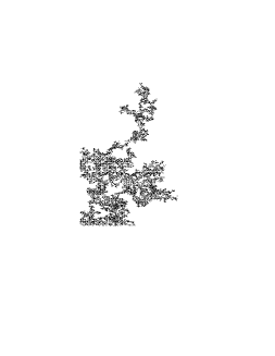
FIG. 2.: This picture shows the entire cluster. The region of interest in which statistics is taken is the lower-left one.

FIG. 3.: Behavior of the fractal dimension of the intersection set of IP without trapping versus the normalized distance $z/L$ from the boundary ($H=4$). $z$ and $L$ are in lattice units, then the normalized distance is dimensionless.

FIG. 4.: Collapse plot of $[d(z)-d^{sur}]log(L)$ for the different sizes, in $log-linear$ scale, for IP without trapping ($H=4$). $z$ and $L$ are in lattice units, then the normalized distance is dimensionless.

FIG. 5.: Behavior of the fractal dimension of the intersection set of IP with trapping versus the normalized distance $z/L$ from the boundary ($H=4$). $z$ and $L$ are in lattice units, then the normalized distance is dimensionless.

FIG. 6.: The histogram distribution of bulk perimeter variables in IP without trapping is compared with the distribution of variables near the boundary of the system, after $5\times 10^{3}$ time steps. The two distributions coincide.

FIG. 7.: Border avalanche distribution of IP without trapping in $log-log$ scale. The least square fit gives a slope $\tau^{sur}=1.56\pm 0.05$.

FIG. 8.: Fine graining transformation for occupied cells.

FIG. 9.: The growth column used in the FST scheme. The thick bond is the initiator of the avalanche, with $x=x_{c}$, and the dashed bonds are the bonds of the perimeter after the initiator’s growth.

FIG. 10.: A possible path of growth at the $6^{th}$ order. The invasion proceeds along the arrows, from one black point to another one. The number near each arrow is the growth time.

FIG. 11.: The power law fit we used to get the extrapolated value of $d^{sur}$ for IP without trapping.

FIG. 12.: Extrapolation of the FST fractal dimension $d_{tr}^{sur}$for IP with site trapping.

FIG. 13.: (a)-(b): Boundary conditions for a boundary avalanche after the growth of the initiator. ( ($\bullet$) indicates the cluster sites and ($\circ$) the perimeter ones: the filled segments are grown bonds and the dotted ones are the descendant of the initiator. The left boundary is shown. Its effect is to reduce the maximum number of perimeter bonds in which the avalanche can go (2), with respect to the bulk (3).

REFERENCES

- [1] D. Wilkinson, J. F. Willemsen J. Phys. A London, 16 3365 (1983).
- [2] R. Cafiero, A. Gabrielli, M. Marsili and L. Pietronero Phys. Rev. E 54 1406 (1996).
- [3] R. Chandler, J. Koplik, K. Lerman and J. Willemsen J. Fluid Mech. 119 249 (1982).
- [4] D. Stauffer and A. Aharony, Introduction to Percolation Theory Taylor and Francis, London, Washington, DC (1992).
- [5] M. Paczuski, P. Bak and S. Maslov, Phys. Rev. E 53,414 (1996).
- [6] P. Bak and K. Sneppen, Phys. Rev. Lett. 71, 4083 (1993).
- [7] K. Sneppen, Phys. Rev. Lett. 69, 3539 (1992).
- [8] K. Binder, “Phase Transitions and Critical Phenomena”, Vol. 8, ed. by C. Domb and J.L. Lebowitz (London, Academic), p. 1, (1993).
- [9] A. L. Stella, C. Tebaldi and G. Caldarelli Phys. Rev. E 52 72 (1995).
- [10] G. Caldarelli, C. Tebaldi and A. L. Stella Phys. Rev. Lett. 76 4983 (1996).
- [11] “Finite Size Scaling”, ed. by J. L. Cardy (Amsterdam, North-Holland), (1988).
- [12] J. L. Cardy, Nucl. Phys. B240, 514, (1984).
- [13] C. Vanderzande and A. L. Stella, J. Phys. A 20, 3001, (1987).
- [14] M. Marsili J. Stat. Phys. 77 733 (1994); A. Gabrielli, M. Marsili, R. Cafiero and L. Pietronero J. Stat. Phys. 84, 889 (1996).
- [15] A. Erzan, L. Pietronero and A. Vespignani Rev. Mod. Phys. 67 n.3 (1995).
- [16] R. Cafiero, G. Caldarelli and A. Gabrielli, Phys. Rev. E, 56 R1291 (1997).
- [17] M. Sahimi, Flow and Transport in Porous Media and Fractures Rock, VCH Weinheim Germany (1995).
- [18] S. Maslov, Phys. Rev. Lett. 74, 562 (1995).
- [19] L. Niemeyer, L. Pietronero and H. J. Wiesmann, Phys. Rev. Lett., 52, 1033 (1984)