Field Theory of Mesoscopic Fluctuations in Superconductor/Normal-Metal Systems

Abstract

Thermodynamic and transport properties of mesoscopic conductors are strongly influenced by the proximity of a superconductor: An interplay between the large scale quantum coherent wave functions in the normal mesoscopic and the superconducting region, respectively, leads to unusual mechanisms of quantum interference. These manifest themselves in both the mean and the mesoscopic fluctuation behaviour of superconductor/normal-metal (SN) hybrid systems being strikingly different from those of conventional mesoscopic systems. After reviewing some established theories of SN-quantum interference phenomena, we introduce a new approach to the analysis of SN-mesoscopic physics. Essentially, our formalism represents a unification of the quasi-classical formalism for describing mean properties of SN-systems on the one hand, with more recent field theories of mesoscopic fluctuations on the other hand. Thus, by its very construction, the new approach is capable of exploring both averaged and fluctuation properties of SN-systems on the same microscopic footing. As an example, the method is applied to the study of various characteristics of the single particle spectrum of SNS-structures.

Contents

toc

I Introduction

Physical properties of both superconductors and mesoscopic normal metals are governed by mechanisms of macroscopic quantum coherence. Their interplay in SN-systems, i.e. hybrid systems comprised of a superconductor adjacent to a mesoscopic normal metal, gives rise to qualitatively new phenomena (see Ref. [1] for a review): Aspects of the superconducting characteristics are imparted on the behaviour of electrons in the normal region. This phenomenon, known as the “proximity effect”, leads to both the mean (disorder averaged) properties of SN-systems being substantially different from those of normal metals and various types of mesoscopic fluctuations.

Although these two classes of phenomena are rooted in the same fundamental physical mechanism – a tendency towards the formation of Cooper pairs in the normal metal region of a SN-system – there are also major differences. Even so, it is notable that more than two decades passed between the first analyses of the manifestations of the proximity effect in the mean properties of SN-systems and the mere observation that the same effect may also be exhibited in mesoscopic fluctuations. The intimate connection between mean and fluctuation manifestations of the proximity effect will be discussed in some detail below. At this stage we simply itemize some basic proximity effect induced phenomena – of both mean and fluctuation type – and briefly comment on the theoretical approaches that have been applied to their analysis.

Mean properties of SN-systems: Superconductors strongly modify the physical properties of adjacent normal metals. For example, the proximity of a superconducting condensate tends to induce singular behaviour in the normal metal density of states (DoS). The properties of these singularities depend on both the coupling to the superconductor and purely intrinsic characteristics of the normal mesoscopic component. This complex behaviour indicates that we are confronted with an interplay between mechanisms of quantum coherence in the superconductor and in the mesoscopic N-region. DoS singularities are only one of many more examples of manifestations of the proximity effect. For example, supercurrents may flow through normal metal regions and the conductance of the normal metal may vary with the phase of the superconducting order parameter [2, 3, 4]. Indeed the conductance may, quite counterintuitively, increase as a function of the impurity concentration, through the phenomenon known as reflectionless tunneling [1, 5].

All these phenomena share the common drawback that they are exceedingly difficult to describe within conventional perturbative techniques of condensed matter physics. Broadly speaking, the reason for these problems is that the conventional ’reference point’ of perturbative approaches to dirty metals, i.e. a filled Fermi sea of electrons with an essentially structureless dispersion relation, represents a poor starting point to the description of SN-hybrids. In fact, the proximity of a superconductor leads to a strong modification of the states in the vicinity of the Fermi-surface, which implies that it is difficult to perturbatively interpolate between the conventional weakly disordered metal limit and the true state of the N-component of a SN-system.

In the late sixties, Eilenberger [6] also introduced a novel approach to the description of bulk superconductors which subsequently turned out to be extremely successful in the analysis of SN-systems. Essentially this so-called quasi-classical approach provided a controlled coarse-graining procedure by which the Gorkov equation for the microscopic Green function of superconductors could be drastically simplified. Since on the one hand the Green function contains all the information that is needed to describe SN-phenomena, whilst on the other hand – for the reasons indicated above – its computation in proximity effect influenced environments is in general tremendously difficult, it is clear that Eilenberger’s method represented a breakthrough. Extending Eilenberger’s work, Usadel [7] later derived a non-linear, diffusion-type equation for the quasi-classical Green function of dirty metals (for the precise definition of the term ’dirty’, see below), the so-called Usadel equation. Based largely on the pioneering work of Eilenberger [6] and Usadel [7], a powerful array of quasi-classical methods has since been developed to study the mean properties of SN-systems.

In view of what has been said above about the difficulties encountered in perturbative approaches, it is instructive to re-interpret the solution of the quasi-classical equations in terms of the language of conventional diagrammatic perturbation theory. Referring for details to later sections, we here merely notice that the quasi-classical Green functions actually represent high-order summations of quantum interference processes caused by multiple impurity scattering. More precisely, the solution of the Usadel equation generally sums up infinitely many so-called diffuson diagrams, the fundamental building blocks of the perturbative approach to dirty metals. Whereas in normal metals high order interference contributions to physical observables are usually small in powers of the parameter $g^{-1}$ ($g\gg 1$ is the dimensionless conductance of a weakly disordered metal), here they represent the leading order contribution even to a single Green function. In passing we note that, very much as the conductance of normal metals may be expanded in terms of the weak localization corrections, disorder averaged properties of SN-systems can be systematically expanded beyond the leading quasi-classical approximation in powers of $g^{-1}$. We will come back to this issue below. Having made these observations one may anticipate that the tendency to strong quantum interference in SN-systems not only affects their mean properties but also leads to the appearance of unusual mesoscopic fluctuation behaviour.

Mesoscopic fluctuations: It has been shown both experimentally [8, 9] and theoretically [2, 3, 10, 11, 13, 14, 15, 16, 18, 19] that mesoscopic fluctuations in SN-systems not only tend to be larger than in the pure N-case, but also can be of qualitatively different physical origin. After what was said above it should be no surprise that the pronounced tendency to exhibit fluctuations again finds its origin in an interplay between standard mechanisms of mesoscopic quantum coherence and the proximity effect.

The list of examples of such SN-specific mesoscopic fluctuation phenomena includes

• As in N-systems, sample-specific fluctuations of the conductance are universal. However, due to proximity effect induced coherence mechanisms, the fluctuations are generally larger than in normal systems [8, 9].

• Besides the normal current, the critical Josephson current, $I_{c}$, through SNS-junctions exhibits fluctuations [3], which become universal in the limit of a short ($L\ll\xi$) junction [20]:

  $$\langle\delta I_{c}^{2}\rangle\sim\left\{\begin{array}[]{lc}(eE_{c})^{2},&L\gg\xi,\\ (e\Delta)^{2},&L\ll\xi.\end{array}\right.$$

  Here $\xi=(D/\Delta)^{1/2}$ is the coherence length of dirty superconductors, $\Delta$ the order parameter, $D$ the diffusion constant, $E_{c}=D/L^{2}$ the Thouless energy and $L$ the system size (note that we set $\hbar=1$ throughout).

• Such fluctuations of the supercurrent are relatively robust [3]: for instance, a relatively strong magnetic field will exponentially suppress the average supercurrent, but reduces the variance of the supercurrent fluctuations by only a factor of 2.

• The single particle spectrum in the vicinity of the DoS anomaly exhibits characteristic types of statistics [10, 19].

• Novel types of universal spectral fluctuations appear [10].

As compared to the mean properties of SN-systems, the physics of fluctuation phenomena is less well understood. Firstly, the quasiclassical approach is not tailored to an analysis of fluctuations. Although, to compute fluctuations, one needs to average products of Green functions over disorder, the quasiclassical equations are derived for single disorder averaged Green functions and can, to the best of our knowledge, not be extended to the computation of higher order cumulants. Secondly, diagrammatic methods, for reasons similar to those outlined above, are ruled out in cases where the proximity effect is fully established.

Important progress has been made by extending the scattering formulation of transport in N-mesoscopic systems to the SN-case [21, 11, 22, 23]. This approach made possible an efficient calculation of both fluctuation and weak localization contributions to various global transport properties of SN-systems [1]. Unlike the quasiclassical formalism, however, the transfer matrix approach is not microscopic. Instead, the different components of an SN-system are treated as black boxes which are described in terms of phenomenological stochastic scattering matrices. This approach, whilst extremely powerful in the analysis of global transport features (the conductance say), cannot address problems that necessitate a local and truly microscopic description. For example, it is not suitable for the calculation of spectral fluctuations, both global and local, the analysis of local currents, and so on.

The purpose of this paper is to introduce a theoretical approach to the study of SN-systems which essentially represents a unification of the above quasiclassical concepts with more recent field theoretical methods developed to study N-mesoscopic fluctuations. As a result we will obtain a modelling of SN-systems that treats mean and fluctuation manifestations of the proximity effect on the same footing, thereby revealing their common physical origin. This work represents the development of ideas that we have originally presented in a short letter [12].

Our starting point will be a connection, recently identified, between quasiclassical equations for Green functions on the one hand and supersymmetric nonlinear $\sigma$-models on the other. As was shown by Muzykhantskii and Khmelnitskii [24], the former can be regarded as the classical equations of motions of the latter. In other words, the $\sigma$-model formulation has been shown to provide a variational principle associated to quasiclassics. So far, these connections have not been exploited within their natural context, superconductivity. To fill this gap, we will demonstrate here that by embedding concepts of quasiclassics into a field theoretical framework, one obtains a flexible and fairly general theoretical tool to the analysis of SN-systems. In particular, it will be straightforward to extend the quasiclassical equations so as to account for the consequences of time-reversal symmetry, the connections to perturbative diagrammatic approaches will become clear, and – most importantly – the effective action approach may be straightforwardly extended to the computation of mesoscopic fluctuations. In doing so, it will become clear in which way both the characteristic features of the Usadel Green function and SN-mesoscopic fluctuations originate in the same basic mechanisms of quantum interference.

In this paper the emphasis will be on the construction of the approach, that is, most of its applications will be deferred to forthcoming publications. However, in order to demonstrate the practical use of the formalism we will consider at least one important representative of mesoscopic fluctuation phenomena, namely fluctuations in the quasi-particle spectrum, in some detail: The DoS of N-mesoscopic systems exhibits quantum fluctuations around its disorder averaged mean value which may be described in terms of various types of universal statistics. The analogous question for SN-systems – What types of statistics govern the disorder induced fluctuation behaviour of the proximity effect influenced DoS? – has not been answered so far. Below we will show the emergence of some kind of modified Wigner Dyson statistics[25], within the newly constructed formalism. A concise presentation of both the field theory and its application to SNS-spectral statistics is contained in Ref. [12].

The organization of the paper is as follows. In section II, we review the basic microscopic mechanism responsible for SN-quantum interference phenomena. In section III, we discuss the quasiclassical approach to the computation of single particle Green functions. In section IV, we briefly review the diagrammatic and statistical scattering approaches as the only methods so far developed to compute mesoscopic fluctuations. In the central sections V-VII, we introduce the aforementioned field theoretical framework. In section V, we derive the effective action for a diffusive SN-structure in the form of a supersymmetric nonlinear sigma-model. In section VI, we obtain the saddle-point equations of the action and examine their solution for some simple geometries. As mentioned above, these saddle-point equations, obtained by a stationary phase analysis of the effective action, are none other than the quasiclassical equations of motion. In section VII, we address the central issue of this paper, the behaviour of fluctuations around the saddle-point solutions. The action displays a spontaneous breaking of symmetry, whose massless, or Goldstone modes are the diffusion modes of the system. The interaction of the diffusion modes is incorporated naturally within this formalism, despite their strong modification due to the proximity effect, and leads to mesoscopic fluctuations. We calculate in this section the renormalization of the spectrum of a quasi-1D SNS junction due to such fluctuations. We also demonstrate the spectral statistics of the SN structure to be described at low energies by a modified version of a universal Wigner-Dyson, or random matrix theory. The field theoretic formalism will also allow us to examine the onset at higher energies of non-universal corrections which serve to destroy the correlations described by such a universal model. In section VIII, we conclude with a discussion.

II Andreev Reflection and the Proximity Effect

Consider a normal metal at mesoscopic length scales, that is, scales much less than both $L_{\varphi}$ and $L_{T}$, where $L_{\varphi}$ is the dephasing length due to electron-electron interactions and $L_{T}=(T/D)^{1/2}$ sets the scale at which the quantum mechanical coherence is cut off by thermal smearing effects. The interest of such mesoscopic materials stems from the fact that their physical behaviour is strongly influenced by effects of large scale quantum interference. Such effects manifest themselves in both a variety of fluctuation phenomena and (non-stochastic) quantum corrections to physical observables.

At the same time, the physics of bulk superconductors is also determined by mechanisms of macroscopic quantum coherence. For example, the Cooper pairs forming a superconducting condensate represent two-electron states whose phase coherence extends over a (possibly macroscopic) scale set by the superconducting coherence length.

Given that the physics of both mesoscopic metals and bulk superconductors is influenced by quantum coherence, it is appropriate to expect that novel interference mechanisms arise when two systems of this type are combined. This is indeed what happens and has led to the continued interest in the physics of SN-hybrid systems. A key piece of information required for the understanding of large scale manifestations of SN-quantum coherence is the manner in which normal metals and superconductors exchange quantum phase information on a microscopic level. The basic coupling mechanism between a superconductor and normal metal is a form of interface scattering, known as Andreev reflection [26, 27]. In this process, depicted in figure 1(a), an electron at an energy below the superconducting gap, $\Delta$, strikes the SN-interface. Due to its low excitation energy it represents a forbidden quasi-particle state and is unable to enter the S-region. Instead, however, it may be Andreev reflected off the boundary as a hole. As a result two excess charges are left at the interface which disappear into the superconducting condensate as a Cooper pair.

$\displaystyle\begin{array}[]{ccc}\psfig{height=99.58464pt}&&\psfig{height=99.58464pt}\\ {\em(a)}&&{\em(b)}\end{array}$

FIG. 1.: (a) Andreev reflection of an electron at an SN interface, and (b) a typical pair of Feynman paths that lead to a non-zero value of $\langle\psi^{\dagger}\psi^{\dagger}\rangle$.

The detailed physics of Andreev scattering and its consequences for SN structures has been reviewed extensively in the literature (see e.g. [1, 26, 28, 29, 30, 31]). Here we merely summarize some of its essential features that will be of importance throughout:

• As opposed to ordinary specular reflection, Andreev-reflection represents a process of ’retro-reflection’. More precisely, apart from a slight angular mismatch proportional to the excitation energy, $\epsilon$, of the electron above the Fermi energy, $\epsilon_{F}$, the hole is reflected back along the trajectory of the incoming electron.

• An electron with excitation energy $\epsilon$ is scattered into a hole with energy $-\epsilon$.

• The hole acquires a scattering phase $\pi/2-\varphi$, where $\varphi$ is the phase of the superconducting order parameter at the interface.

An important consequence of the existence of the Andreev scattering mechanism is the formation of a Cooper-pair amplitude $\langle\langle\psi^{\dagger}({\bf x})\psi^{\dagger}({\bf x})\rangle\rangle$ in the normal metal region. Here $\langle\langle\ldots\rangle\rangle$ not only represents the quantum mechanical expectation value but also a disorder average. The creation of an average local pairing amplitude can be heuristically understood from a simple semiclassical consideration: Consider the creation of an electron somewhere at a point ${\bf x}$ inside a disordered metal adjacent to a superconductor (see fig. 1(b)). Due to the presence of disorder, the electron will propagate diffusively and may eventually strike the SN-interface and be Andreev reflected. In general the newly created hole may now diffuse along its own path. However, a particularly interesting situation arises if the hole happens to propagate along the path of the incoming electron back to the point of creation. As a result we obtain a non-vanishing pairing field amplitude $\langle\langle\psi^{\dagger}({\bf x})\psi^{\dagger}({\bf x})\rangle\rangle$. The point is that during their propagation through the disordered background both the incoming electron and the outgoing hole accumulate a quantum mechanical scattering phase which depends sensitively on microscopic details of the disorder. However, owing to the fact that the two particles propagate along the same path these phases cancel each other to a large extent. (For an excitation energy $\epsilon=0$ the cancellation is, in fact, perfect. For non-vanishing $\epsilon$ one obtains a phase mismatch $\sim L_{\rm p}\epsilon/v_{F}\propto\epsilon L^{2}/D$, where $L_{\rm p}$ is the length of the scattering path, $D$ the diffusion constant, $v_{F}$ the Fermi velocity, $L$ the separation of ${\bf x}$ from the interface and we have used the fact that for diffusive motion $L_{\rm p}/v_{F}\propto L^{2}/D$.) Of course, while more generic path pairs, where the electron and hole follow different paths, also contribute to $\langle\psi^{\dagger}({\bf x})\psi^{\dagger}({\bf x})\rangle$, their contributions vanish upon disorder averaging due to their strong phase dependence.

The non-vanishing of $\langle\langle\psi^{\dagger}({\bf x})\psi^{\dagger}({\bf x})\rangle\rangle$ is the basic content of the proximity effect. Besides its resilience against disorder, the pairing field amplitude possesses a number of important features – all of which are related to the phase argument above – that will be of importance for all that follows:

• $\langle\langle\psi^{\dagger}({\bf x})\psi^{\dagger}({\bf x})\rangle\rangle$ varies weakly as a function of ${\bf x}$. More precisely, it does not fluctuate on atomic scales but rather on scales set by $(D/\epsilon)^{1/2}$.

• $\langle\langle\psi^{\dagger}({\bf x})\psi^{\dagger}({\bf x})\rangle\rangle$ decays exponentially as a function of $\epsilon L^{2}/D$. If either $T$ or the inverse dephasing time $\tau_{\varphi}^{-1}$ exceed $\epsilon$, the decay rate is set by these energy scales.

• Quantitative expressions for the diffusive pairs of quantum paths entering the physics of the proximity effect are provided by so-called diffuson modes. Their meaning in the present context will become clear below.

• The pairing field amplitude depends on the phases of the order parameters of the adjacent superconductors. If only a single superconducting terminal with constant phase, $\varphi$, is present, the phase dependence is simply $\sim\exp(i\varphi)$. In this case the phase is inessential and can be eliminated by means of a global gauge transformation. More interesting situations arise when more than one superconductor are present, in which case the phase sensitivity of the pairing amplitude provides the mechanism for the stationary Josephson effect.

The non-vanishing of the pairing field amplitude heavily influences the properties of the normal metal components of SN-systems. Widely known examples of proximity effect induced phenomena are the DC and AC Josephson effect, which allow the possibility of supercurrent flows through SNS-sandwiches. Another important phenomenon is the dependence of the N-conductance on the phases of adjacent superconductors – again triggered by the phase sensitivity of the proximity amplitude [4, 34]. However, as mentioned in the introduction, the emphasis in this paper will be on a study of the influence of the proximity effect on the single particle spectrum.

A Single-Particle Spectrum

To understand the basic connection between the proximity effect and the single particle spectrum, let us begin by considering the simple geometry of an SNS-sandwich, shown in fig. 2, where the N-layer is of width $L$, of otherwise infinite extent and clean. This system was first considered by Andreev [26] who applied scattering theory to the electron wavefunction to show that the spectrum in the N region, for trajectories at a fixed angle to the interface, is discrete below the superconducting gap. The ’Andreev levels’ correspond to bound states with energies $\epsilon$ given by the quantization rule,

$$\tan\left(\frac{\epsilon L}{|v_{x}|}+{\rm sgn}(v_{x})\frac{\Delta\varphi}{2}\right)=\frac{\sqrt{\Delta^{2}-\epsilon^{2}}}{\epsilon},$$ (2)

where $\Delta\varphi$ the phase difference across the junction and $v_{x}$ the component of the electron velocity normal to the interface. Eq. (2) then indicates an average Andreev level spacing of the order of the inverse flight time, $|v_{x}|/L$, across the normal region. A non-zero phase difference, $\Delta\varphi$, leads to a shift in the levels so as to produce two separate branches of the spectrum, for electrons and holes respectively.

FIG. 2.: The geometry of the SNS junction.

To determine the observed spectrum, it is necessary to sum the pole contributions to the DoS from bound states which arise from all possible velocity directions, according to Eq. (2). Note that non-zero contributions survive down to arbitrarily small energies due to trajectories travelling close to parallel to the interface. The energy dependence of the weights of these poles is so as to produce a total DoS which is linear in energy $\epsilon$, at energies $\epsilon\ll\Delta$.

The introduction of a finite concentration of impurities leads, upon disorder averaging, to a smearing of the formerly sharp pole structure. A less obvious outcome of this process is the appearance of a sharp cut-off in the spectrum, the ’minigap’, below which the DoS vanishes entirely. The minigap, $E_{g}$, is smaller than the superconducting gap, $\Delta$, and depends on $\Delta\varphi$, attaining its maximum for $\Delta\varphi=0$ and shrinking to zero as $\Delta\varphi$ approaches $\pi$. In general $E_{g}$ depends on $\Delta\varphi$ in a non-sinusoidal fashion [35], although in the limit of a short, diffusive junction, $L\ll\xi$, the dependence becomes sinusoidal, $E_{g}=\Delta\cos(\Delta\varphi/2)$ [36].

In the general case, the formation of a minigap in the metallic DoS represents a highly non-trivial phenomenon. For example, it has been shown [37] that the presence or absence of a gap depends on the classical dynamical features of the metallic probe contacting the superconductor: For samples with integrable classical dynamics (such as the cubic system described above) there is no gap but rather a DoS that vanishes linearly at the Fermi energy. The existence of states all the way down to zero energy may be understood by means of Bohr-Sommerfeld quantization arguments. By contrast, in systems with chaotic classical dynamics, a gap opens whose magnitude may depend on both the coupling strength to the superconductor and the intrinsic classical transport time through the metal region.

B Failure of Semiclassics: Quantum Diffraction

The prediction of a minigap provides a useful test for any analytic approach to the physics of SN-systems: for example, an application of standard approximation schemes to semiclassical formulae for the the DoS fails to predict correctly a gap.

To explain this point, let us consider the simple case of a diffusive metallic cube of linear extension $L$ attached to a superconductor. In this case the DoS gap is of width $\simeq E_{c}$. In order to embed the previous heuristic path arguments regarding the proximity effect into a quantitative calculation of the proximity effect influenced DoS one might apply the semiclassical Gutzwiller trace formula [38], a powerful computational tool often used in the analysis of the DoS and correlations thereof. The Gutzwiller trace formula essentially states that the averaged DoS can be obtained as a sum over all periodic orbits with vanishing, or at least a disorder insensitive action [39]. Small action contributions to trace formulae are usually computed from the so-called diagonal approximation. In the present context the diagonal approximation would amount to counting Feynman paths such as the one depicted in fig. 3(a). (The smallness of the action of these pairs of paths follows from the fact that if the action of the electronic segment of the path (solid line) has an energy dependent action $S(\epsilon)$, the action of the hole segment (dashed line) will be $-S(-\epsilon)$. The two contributions nearly cancel each other.)

The problem with the standard diagonal approximation is that it fails to predict a gap in the DoS, even if paths with multiple Andreev scattering are taken into account. In order to understand this failure we first have to notice that small action path-pairs exist which do not fall into the scope of the diagonal approximation (by which we mean that they cannot be obtained as a superposition of two identical segments, one electron- one hole-like). A common feature of these ’non-diagonal’ path configurations is that they contain ’junction points’ were the paths of electrons and holes split (cf. fig. 3(b)). In order to understand the existence of these splittings one has to keep in mind that the paths entering the semiclassical picture do not correspond to rigorously defined solutions of classical equations of motion but should rather be thought of as objects that are smeared out (in configuration space) over scales comparable with the Fermi wavelength [40]. As a result two classically ’identical’ paths may split and recombine at some later stage, a process which is not accounted for by the diagonal approximation. This splitting, as it is caused by the wave nature of the electrons, is sometimes referred to as a quantum diffraction phenomenon.

Note that the junctions appearing in fig. 3(b) are reminiscent of similar processes needed to generate weak localization corrections to the conductance of normal metals [40]. However, whereas weak localization corrections represent a correction of ${\cal O}(g^{-1})$ to the classical conductance ($g\gg 1$ is the dimensionless conductance), the diffraction corrections appearing in the present context can by no means be regarded as small. In fact they are as important as the leading order diagonal contributions which implies that processes with up to an infinite number of ’junction points’ have to be taken into account. This fact not only explains the failure of the diagonal approximation but also the difficulties encountered in diagrammatic analyses of the proximity effect. The point is that each of the ’legs’ appearing in fig. 3(b) represents a Cooperon. The perturbative summation of infinitely many Cooperons represents a difficult problem, in particular in cases where the sytem is truly extended in the sense that it cannot be treated within an ergodic or zero mode approximation (for a perturbative analysis of the zero-mode scenario, see Brouwer et al., [41]). Fortunately there is an alternative approach, the quasiclassical method reviewed below, which provides a highly efficient tool for the effective summation of all interference corrections contributing to the DoS and other physical observables.

$\displaystyle\begin{array}[]{ccc}\psfig{height=99.58464pt}&&\psfig{height=99.58464pt}\\ {\em(a)}&&{\em(b)}\end{array}$

FIG. 3.: Trajectories that are (a) included and (b) not included within a semiclassical treatment.

III Quasiclassics

In order to prepare the discussion of quasiclassics we first need to introduce its microscopic basis in general and the Gorkov Green function in particular.

A The Gorkov Equations

As long as interaction effects are neglected the complete information on any SN-system is encoded in its single particle Gorkov Green function, ${\cal G}^{\rm{r,a}}$. The latter is defined by the Gorkov equations [42], whose matrix representation reads

$$\left(\matrix{\mu+\epsilon_{\pm}-{1\over 2m}\left(\hat{{\mathbf{p}}}-{e\over c}{\mathbf{A}}({\mathbf{r}}_{1})\right)^{2}-\hat{V}({\mathbf{r}}_{1})&\Delta({\mathbf{r}}_{1})\cr-\Delta({\mathbf{r}}_{1})^{*}&\mu-\epsilon_{\pm}-{1\over 2m}\left(\hat{{\mathbf{p}}}+{e\over c}{\mathbf{A}}({\mathbf{r}}_{1})\right)^{2}-V({\mathbf{r}}_{1})\cr}\right){\cal G}^{\rm r,a}({\mathbf{r}}_{1},{\mathbf{r}}_{2})$$ (3)

$$\hskip 56.9055pt=\openone\delta^{d}({\mathbf{r}}_{1}-{\mathbf{r}}_{2}),$$ (4)

where

$${\cal G}^{\rm r,a}=\left(\matrix{G^{\rm r,a}&F^{\rm r,a}\cr{F^{\dagger}}^{\rm r,a}&{G^{\dagger}}^{\rm r,a}}\right).$$ (5)

Here $G^{\rm r,a}$ and $F^{\rm r,a}$ represent the normal and anomalous Green function, respectively, $\Delta({\mathbf{r}})$ is the superconducting order parameter (which, in principle, has to be determined self-consistently), $\epsilon_{\pm}=\epsilon\pm i0$, and $V$ is the impurity potential.

The equation above may be represented in a more convenient way by introducing Pauli-matrices, $\sigma_{i}^{\rm ph}$, operating in the two-component particle/hole space. Separating the order parameter into its modulus, $|\Delta({\mathbf{r}})|$, and phase, $\varphi({\mathbf{r}})$, Eq. (3) takes the form

$$\left[\epsilon_{F}-{1\over 2m}\left(\hat{{\mathbf{p}}}-{e\over c}{\mathbf{A}}({\mathbf{r}})\sigma_{3}^{\rm ph}\right)^{2}-V({\mathbf{r}})+\left(\hat{\Delta}({\mathbf{r}}_{1})+\epsilon_{\pm}\right)\sigma_{3}^{\rm ph}\right]{\cal G}^{\rm r,a}({\mathbf{r}}_{1},{\mathbf{r}}_{2})=\delta^{d}({\mathbf{r}}_{1}-{\mathbf{r}}_{2}),$$ (6)

where $\hat{\Delta}=\sigma_{1}^{\rm ph}|\Delta|e^{-i\varphi({\mathbf{r}}_{1})\sigma_{3}^{\rm ph}}$. The presence of an impurity potential, $V({\mathbf{r}})$, makes the solution of Eq. (6) difficult. However, as pointed out by Eilenberger [6] and Larkin and Ovchinnikov [43], a crucial simplification applies in the case where the wavelength of the electrons, $\lambda_{F}$, is small as compared to the characteristic scales over which the order parameter $\Delta({\mathbf{r}})$ and vector potential ${\mathbf{A}}({\mathbf{r}})$ vary. Under this condition one can resort to the ’quasiclassical approximation’.

B Quasiclassical Approximation

The starting point of the quasiclassical approach is the observation that the spatial structure of the Green function is comprised of rapid oscillations, over a spatial scale of the Fermi wavelength, modulated by a slowly fluctuating background over longer scales. A quasiclassical analysis of the proximity effect involves an averaging over the rapid variations of the Green function. At the same time, sufficient information is retained within the slower modes of the Green function to provide a useful approximation to the full consequences of the proximity effect. The advantage is a great simplification of the corresponding kinetic equations. As the derivation of the quasiclassical equations has been reviewed extensively in the literature (e.g. [44, 31, 49]), we restrict ourselves here to a brief summary of the main results of the approach.

The quasiclassical, or Eilenberger, Green function, $g^{\rm r,a}({\mathbf{n}},{\mathbf{r}})$, is obtained from the Gorkov Green function by a) a Wigner transform, b) an impurity average and c) an integral over the kinetic energy variable. The precise definition reads

$$g^{\rm r,a}({\mathbf{n}},{\mathbf{r}})=\frac{i}{\pi}\int d\xi\int d({\mathbf{r}}_{1}-{\mathbf{r}}_{2}){\mathcal{G}}^{\rm r,a}({\mathbf{r}}_{1},{\mathbf{r}}_{2})\exp(-i{\mathbf{p}}\cdot({\mathbf{r}}_{1}-{\mathbf{r}}_{2})),$$ (7)

where ${\mathbf{r}}=({\mathbf{r}}_{1}+{\mathbf{r}}_{2})/2$, $\xi_{p}=v_{F}(p-p_{F})$, ${\mathbf{n}}={\mathbf{p}}/p$ and $p_{F}=mv_{F}$ is the Fermi momentum. The application of this approximation to the Gorkov equation, Eq. (6) leads to the ‘Eilenberger equation’ [6]:

$${\mathbf{v}}_{F}\cdot{\mathbf{\nabla}}_{r}g^{\rm r,a}({\mathbf{n}},{\mathbf{r}})=i\left[\sigma_{3}^{\rm ph}(\epsilon_{\pm}+\hat{\Delta}({\mathbf{r}}))+\frac{i}{2\tau}\left\langle g^{\rm r,a}({\mathbf{n}}^{\prime},{\mathbf{r}})\right\rangle_{{\mathbf{n}}^{\prime}},g^{\rm r,a}({\mathbf{n}},{\mathbf{r}})\right],$$ (8)

where $\tau$ is the elastic scattering time due to impurities. This equation essentially represents an expansion to leading order in the ratio of $\lambda_{F}$ to the scale of spatial variation of the slow modes of the Gorkov Green function. It can be shown that the Eilenberger Green function obeys the nonlinear normalization condition (see, for example, the discussions in Refs.[47, 48])

$$g^{\rm r,a}({\mathbf{n}},{\mathbf{r}})^{2}=\openone.$$ (9)

Eq.(8) represents an equation of Boltzmann-type which is much simpler than the original Gorkov equation, but may still be difficult to solve in general. However, significant further simplifications are possible in the ’dirty limit’.

C Dirty Limit

The ’dirty limit’ is specified by the conditions $\ell=v_{F}\tau\ll\xi$ (implying that the dominant transport mechanism is diffusion) and $\epsilon<\tau^{-1}$ (implying that ’time scales’ $\epsilon^{-1}$ much longer than the scattering time are explored). Under these conditions, the dependence of the Green function on the angular direction (represented by ${\mathbf{n}}$) is weak and one may expand in its first two spherical harmonics:

$$g^{\rm r,a}({\mathbf{v}}_{F},{\mathbf{r}})=g_{0}^{\rm r,a}({\mathbf{r}})+{\mathbf{n}}\cdot{\mathbf{g}}_{1}^{\rm r,a}({\mathbf{r}})+\ldots,$$ (10)

where $g_{0}^{\rm r,a}({\mathbf{r}})\gg{\mathbf{n}}\cdot{\mathbf{g}}_{1}^{\rm r,a}({\mathbf{r}})$. A systematic expansion of the Eilenberger equation in terms of ${\mathbf{g}}_{1}$ then leads to a nonlinear and second-order equation for the isotropic component,

$$D{\mathbf{\nabla}}(g_{0}^{\rm r,a}({\mathbf{r}}){\mathbf{\nabla}}g_{0}^{\rm r,a}({\mathbf{r}}))+i[\sigma_{3}^{\rm ph}(\epsilon_{\pm}+\hat{\Delta}({\mathbf{r}})),g_{0}^{\rm r,a}({\mathbf{r}})]=0,\hskip 14.22636ptg_{0}^{\rm r,a}({\mathbf{r}})^{2}=\openone,$$ (11)

known as the ‘Usadel equation’ [7]. In order to specify a solution, one has to supplement the equation with appropriate boundary conditions. The analysis of the boundary behaviour of the equation becomes somewhat technical. For this reason a more detailed discussion of the boundary conditions

$$\sigma(-)g_{0}\partial_{r}g_{0}(-)=\sigma(+)g_{0}\partial_{r}g_{0}(+)$$ , (13)

$$\sigma(\pm)g_{0}\partial_{r}g_{0}(\pm)=\frac{G_{T}}{2}[g_{0}(+),g_{0}(-)], \qquad T\ll 1,$$ (14)

$$g_{0}(+)=g_{0}(-), \qquad T\simeq 1,$$ (15)

has been made the subject of appendix A. Here $T\in[0,1]$ is a measure for the transparency of the S/N interface, $g_{0}(\pm)$ denotes the Green functions infinitesimally to the left respectively right of the junction, and $G_{T}$ (cf. Eq. (A9)) is the tunnel conductance of the interface.

D Solution of the Usadel Equation

Solutions of the Usadel equation with appropriate boundary conditions have been derived for a vast number of geometries. At the same time a systematic and general solution scheme, based on an effective circuit theory, has been constructed by Nazarov [52]. Furthermore, a number of quasiclassical predictions seem to be borne out well experimentally (see e.g. [34, 53, 54, 55, 56, 57]. In the field theoretic context introduced below, the Usadel equation and its boundary condition will reappear on the level of the mean field analysis in section VI. In addition explicit solutions for some simple geometries will be discussed in that section.

It is instructive to consider a diagrammatic reinterpretation of the Usadel solution in terms of a summation over real-space trajectories. Such a decomposition may be achieved by taking the solution of Eq. (11) in a normal region, with the SN interface (at $x=0$, say) represented (for energies $\epsilon\ll\Delta$) by a boundary, or source, term $\Delta\delta(x)$. An expansion of the solution in powers of $\Delta$ corresponds to a series of diffusive trajectories which include successive numbers of Andreev reflections at the interface. Fig. 3 (b) provides an illustration of a trajectory with four reflections, whilst ’starfish’ trajectories with arbitrary numbers of reflections are clearly possible. The reproduction of the Usadel solution requires the summation of the full set of trajectories, corresponding to diagrams to all orders. We see that the inherent difficulties of a diagrammatic treatment of the proximity effect, as discussed earlier, extend even to the relatively simple task of reproducing quasiclassics.

IV Beyond Quasiclassics

The quasiclassical approach allows for the efficient calculation of a wide spectrum of physical observables. In general, any observable that may be expressed in terms of a single disorder averaged Green function is a candidate for quasiclassical analysis. Note that, by extending the formalism so as to include Keldysh-Green functions [58], observables that are commonly expressed in terms of two-particle Green functions also become accessible. Important examples are the conductance and other transport quantities. However, there are important classes of observables which do not fall into the above category, thereby falling beyond the scope of quasiclassics. The list of inaccessible quantities may be grouped roughly into four different categories:

• Physical observables which, by definition, are not expressible in terms of single particle Green functions. An example is given by the magnetic field dependence of the London penetration depth for a bulk superconductor, as studied by Larkin and Ovchinnikov [43]. Its analysis requires the computation of the average of four momentum operators, $\langle p(0)p(t)p(0)p(t)\rangle$, a quantity that involves two- rather than one-particle Green functions.

• Higher order quantum interference corrections to single particle Green-functions. Very much like weak localization corrections of ${\cal O}(g^{-1})$ to the classical Drude conductance, the quasiclassical Green function represents the leading order term of a series expansion in powers of $g^{-1}$. The next to leading order contributions become important in cases where one is interested in quantum corrections of weak localization type or strong localization effects.

• The quasiclassical approach (in its extension to include a Keldysh component) does not account for the corrections to two-particle Green functions due to the interference of mutually time-reversed trajectories. An example property that is affected in this way is the conductivity, as we see below.

• Most importantly, the quasiclassical approach does not allow for the study of mesoscopic fluctuation phenomena. The analysis of fluctuations requires the computation of disorder averages of two or more Green functions. Due to the impurity induced interference between different Green functions, quasiclassical techniques are inapplicable to these problems.

Given that these classes of problems cannot be addressed within quasiclassics, it becomes necessary to seek some alternative approach. Here, we briefly review two of perhaps the most important theoretical tools currently established, namely, diagrammatics and the scattering matrix approach.

A Perturbative Diagrammatic Methods

Microscopic diagrammatic methods have been applied to the study of various SN-phenomena. The list of diagrammatic analyses includes computations of Josephson current fluctuations through SNS junctions[3], investigations of the phase sensitivity of the N-conductance[2], computations of universal conductance fluctuations of SN-systems [11] and more.

$$\begin{array}[]{ccc}\psfig{height=170.71652pt}&&\psfig{height=170.71652pt}\\ ({\em a})&&({\em b})\end{array}$$ (18)

FIG. 4.: (a) shows the trajectories whose interference leads to the first weak localization correction to the conductivity. (b) shows the corresponding diagrams, where the curvy line is the cooperon and the triangles represent Andreev reflection processes.

The basic building block of diagrammatic analyses are the diffusion modes both of diffuson and cooperon type. What makes these modes different from their counterparts in pure N-systems is that they now include Andreev scattering events, as represented in fig. 4. In the presence of the proximity effect, any of the Andreev scattering vertices appearing in these modes is in turn to be renormalized by further diffusion modes, as indicated in fig. 5. Note that these diagrams are the formal representation of what in real space are the ’legs’ of the starfish-like structures appearing in fig. 3. The problem with the diagrammatic approach is that in situations where the proximity effect is fully established, the Andreev vertices renormalize heavily, i.e. one has to sum self-consistently nested series of the diagrams depicted in fig. 5. Another way of putting this is to say that one has to perturbatively reconstruct the solution of the Usadel equation, a difficult if not impossible task. In fact, an incomplete account of the proximity-induced renormalization processes may lead to incorrect results: for example, diagrammatic analyses of universal conductance fluctuations by Takane et al. [11] failed to reproduce correctly their surprising insensitivity to external magnetic fields, as later demonstrated by Brouwer et al. [1, 16]. However, in cases where the proximity effect is either suppressed or of secondary importance, diagrammatic tools can be applied successfully to the study of SN-systems.

In summary, it can be said that diagrammatics is applicable to the perturbative analysis of SN-phenomena in cases with a weakly pronounced proximity effect. As is usual with diagrammatic methods, non-perturbative problems, such as localization, fine structure level statistics, and so on, cannot be addressed.

FIG. 5.: First order renormalization of the Andreev scattering process necessary to include the proximity effect.

B Multiple Scattering Formalism

Scattering theory provides a powerful theoretical tool for the analysis of quantum transport through mesoscopic systems in general, and SN-systems in particular. The reason for the efficiency of the scattering theoretical formalism in the study of SN-systems is not only its relative simplicity, but also the fact that the proximity effect does not seem to lead to essential complications. Due to this latter advantage, scattering theory has for a long time existed as the only tool for computing mesoscopic fluctuations under the influence of the proximity effect.

The starting points of the scattering approach are generalizations of the standard multi-channel Landauer formulae for N-mesoscopic systems to the SN-case. For example, in the case of a single N-sample attached to a superconductor the conductance may be expressed as [21, 11, 22]

$$G_{NS}=\frac{2e^{2}}{h}{\rm tr}(1-S_{ee}^{\vphantom{\dagger}}S_{ee}^{\dagger}+S_{he}^{\vphantom{\dagger}}S_{he}^{\dagger})\,=\frac{4e^{2}}{h}{\rm tr}S_{he}^{\vphantom{\dagger}}S_{he}^{\dagger},$$ (19)

where $S_{ee}(S_{eh})$ are the matrices describing the scattering of electrons incoming from the normal metal to electrons (holes). In a next step, the scattering matrices are expressed in terms of a) the transmission matrices of the normal metal compound (which are known in terms of their transmission eigenvalue distribution functions [1, 59], and b) matrices describing the scattering off the superconductor.

The scattering theoretical approach is particularly powerful if the observables of interest take the form of ’linear statistics’, i.e. quantities, $X$, that can be represented as

$\displaystyle X=\sum_{n}f(T_{n}),$

where $f$ is some function and $T_{n}$ is related to the $n$-th normal transmission matrix eigenvalue. This is often but not always the case: for example, in time reversal invariant cases, the conductance of the above SN-system may be formulated as (see Beenakker, [23])

$$G_{NS}=\frac{4e^{2}}{h}\sum_{n=1}^{N}\frac{T_{n}^{2}}{(2-T_{n})^{2}}.$$ (20)

However, if time reversal invariance is broken, such a simple representation is no longer possible and expressions involving not only eigenvalues but also the diagonalizing matrices appear. It has been shown by Brouwer et al. [41] that, even under these more complicated circumstances, scattering theory remains applicable. What becomes necessary is to supplement the conventional transfer matrix approach (by which we mean the derivation and solution of a Fokker-Planck equation for the eigenvalues) by diagrammatic methods accounting for the presence of the diagonalizing matrices. Due to the complex structure of the diagrammatic series appearing in the SN-problem, only quantum dots (i.e. ergodic systems that can be modeled in terms of a scattering matrix distributed through a single Haar measure) rather than arrays thereof could be analyzed in this way: we again encounter the notorious difficulties accompanying perturbative approaches to SN-systems.

In passing we note that in some cases SN-quantum dots, chaotic or disordered, can be modeled in terms of simple random matrix theory. More precisely, random matrix techniques become applicable if the proximity effect is suppressed. This happens if the system is subject to a magnetic field (of the order of a few flux quanta through the system), or if the phases of the adjacent superconductors average to zero. In spite of the fact that the proximity effect is suppressed, the mechanism of Andreev scattering remains active and manifests itself in the SN-random matrix ensembles having symmetry properties that differ substantially from the standard Wigner Dyson ensembles.

To summarize, statistical scattering theory represents a powerful tool for the analysis of both mean and fluctuation characteristics of global transport quantities. Clearly, observables belonging to this category are of outstanding importance from the experimental point of view. Nevertheless, problems remain for which one is interested in observables that are local and/or microscopically defined. This complementary class of quantities is inaccessible through phenomenological scattering analyses. Thus at least one alternative theoretical tool for the analysis of SN systems is called for.

V Field Theory for SN Systems

In the following central part of the paper we are going to introduce a novel approach to the analysis of SN systems which is based on field theoretical and, by construction, microscopic concepts. The formalism will be applicable to observables that can be expressed in terms of one or products of single particle Green functions. If this criterion it met, both mean values (including quantum corrections to quasiclassical results) and mesoscopic fluctuations can be computed. In a few exceptional cases, distribution functions can be obtained. It will quickly turn out that the formalism is intimately related to each of the approaches reviewed above: On the mean field level it reproduces quasiclassics, perturbative fluctuations around the mean field can be interpreted diagrammatically, and the connection to scattering theory is established through general parallels between $\sigma$-models and the transfer matrix approach [65].

Prior to embarking on any kind of detailed discussion, let us briefly outline the main conceptual steps of the construction of the field theory:

1. Starting from the microscopic Gorkov Hamiltonian of an SN-system we will construct a generating functional for the disorder average of the product of a retarded and an advanced Green function. (Generalizations to products of more than two Green functions are straightforward.) The functional will be of a nonlinear $\sigma$-model type. Essentially it represents a supersymmetric extension of earlier (replicated) field theoretical approaches to bulk superconductors[66]. In the present formulation, the order-parameter field will be imposed and not computed self-consistently (a common and mostly inessential simplification in the field of SN-systems).

2. It will then turn out that the spatial inhomogeneity of the order parameter field poses a substantial problem: A straightforward perturbative evaluation of the field theory, by which we mean a perturbative expansion around any spatially homogeneous reference field configuration, is impossible. It goes without saying that this is nothing but the manifestation, in a field theoretical context, of the general perturbative difficulties characteristic to SN-systems.

3. The way out will be to subject the field theory, prior to any perturbative manipulations, to a stationary phase analysis. Given what has been said under the previous item, it is clear that the saddle point configurations of the theory must be spatially inhomogeneous. More specifically it will turn out that the stationary phase equation of the theory is simply the Usadel equation. In other words, the quasiclassical approach to SN-systems turns out to be equivalent to the mean field level of the field theoretical formalism.

4. We then turn to the issue of fluctuations. Broadly speaking, two qualitatively different types of fluctuations will be encountered: Massive fluctuations around the mean field (giving rise to quantum corrections to quasiclassics) and a Goldstone mode. The latter will induce correlations between retarded and advanced Green functions and thereby mesoscopic fluctuations.

To keep the discussion of the above hierarchy of construction steps from being too abstract, the computation of correlations in the single particle spectrum will serve as a concrete example of an application of the theory.

Before turning to the actual construction of the field theory, it should be noted that essential components of the machinery we are going to discuss are not original, but have been introduced earlier: The general supersymmetric field theoretical approach to N-mesoscopic systems has been constructed by Efetov[64]. Oppermann[66], and later Kravtsov and Oppermann[67], introduced a fermion-replicated $\sigma$-model description of bulk disordered superconductors. As far as technical aspects are concerned, the formalism we are deriving represents a supersymmetric extension of Oppermann’s model, tailored to the description of spatially inhomogeneous structures. In its early stages, the construction of the model follows a by now absolutely standard strategy. Essentially, this requires an adaptation of Efetov’s model to allow for the particular structure of Gorkov Green functions. For this reason our presentation of the early construction steps will be concise, but nevertheless self contained.

A Field Integral and the Ensemble Average

As is usual in the construction of field theories of mesoscopic systems, the first construction step is to represent products of matrix elements of Gorkov Green functions in terms of supersymmetric Gaussian field integrals. To keep the discussion comparatively simple, we focus on the case of two-point correlation functions $\langle{\cal G}^{\rm r}(\epsilon+\omega_{+}/2){\cal G}^{\rm a}(\epsilon-\omega_{+}/2)\rangle$ and choose, as a specific example, the quantity

$$\left\langle{\rm tr}_{{\rm ph},{\mathbf{r}}}\left({\cal G}^{\rm r}(\epsilon+\omega_{+}/2)\right){\rm tr}_{{\rm ph},{\mathbf{r}}}\left({\cal G}^{\rm a}(\epsilon-\omega_{+}/2)\right)\right\rangle,$$ (21)

which appears in the computation of the fluctuations of the DoS,

$$R(\epsilon,\omega_{+})=\frac{1}{\langle\nu(\epsilon)\rangle^{2}}\langle\delta\nu(\epsilon+\omega_{+}/2)\delta\nu(\epsilon-\omega_{+}/2)\rangle.$$ (22)

Here $\delta\nu=\nu-\langle\nu\rangle$, $\nu(\epsilon)=-\frac{1}{2\pi}{\rm Im\,}{\rm tr}_{{\rm ph},{\mathbf{r}}}\left({\cal G}^{\rm r}(\epsilon)\right)$ and ${\rm tr}_{{\rm ph},{\mathbf{r}}}$ denotes a trace with respect to both position and particle hole index.

In order to represent objects of this kind in terms of Gaussian field integrals, we first introduce a 16-component vector field, $\psi=\{\psi_{\lambda,s,\alpha,t}({\mathbf{r}})\},\;\lambda,s,\alpha,t=1,2$, with complex commuting (anticommuting) components $\alpha=1\,(\alpha=2)$. The significance of the two-valued indices $\lambda,s,\alpha,t$ is summarized in the following table:

index	significance	abbreviation
$\lambda$	advanced/retarded	ar
$s$	particle/hole	ph
$\alpha$	boson/fermion	bf
$t$	time reversal	tr

Apart from the index $s$ accounting for the $2\times 2$ matrix structure of the Gorkov Green function, all other indices are standard in supersymmetric approaches to disordered systems. For a discussion of their significance we refer to Efetov’s book[64]. We next introduce the action

$$S=-i\int\bar{\psi}\left[\mu-\frac{1}{2m}\left(\hat{{\mathbf{p}}}-\frac{e}{c}{\mathbf{A}}\sigma_{3}^{\rm ph}\otimes\sigma_{3}^{\rm tr}\right)^{2}-V+\sigma_{3}^{\rm ph}\otimes\left(\tilde{\Delta}+\epsilon+{\omega_{+}\over 2}\sigma_{3}^{\rm ar}\right)\right]\psi,$$ (23)

where

$$\tilde{\Delta}({\mathbf{r}})=\Delta\sigma_{1}^{\rm ph}\otimes\sigma_{3}^{\rm tr}\exp(-i\varphi({\mathbf{r}})\sigma_{3}^{\rm ph}\otimes\sigma_{3}^{\rm tr}),$$ (24)

and the Pauli matrices $\sigma_{i}^{\rm ar},\sigma_{i}^{\rm ph},\sigma_{i}^{\rm bf}$, and $\sigma_{i}^{\rm bf},\;i=1,2,3$ operate in the two dimensional spaces of $\lambda,\alpha,s,t$-indices respectively. The fields $\psi$ and $\bar{\psi}$ are related to one another via

$\displaystyle\bar{\psi}=\left(\sigma_{1}^{\rm tr}\otimes E_{11}^{\rm bf}+i\sigma_{2}^{\rm tr}\otimes E_{22}^{\rm bf}\right)\psi,$

where the matrices $E_{ij}^{\rm x},\;{\rm x}={\rm ar,ph,bf,tr}$, are defined as $\left(E_{ij}^{\rm x}\right)_{i^{\prime}j^{\prime}}=\delta_{ii^{\prime}}\delta_{jj^{\prime}}$, and the indices $i^{\prime},j^{\prime}$ refer to the space ${\rm x}$.

As in analogous theories of $N$-systems, the action, $S$, can be employed to represent correlation functions in terms of Gaussian field integrals. Specifically, the expression (21) takes the form

$$\left\langle{\rm tr}_{{\rm ph},{\mathbf{r}}}\left({\cal G}^{\rm r}(\epsilon+\omega_{+}/2)\right){\rm tr}_{{\rm ph},{\mathbf{r}}}\left({\cal G}^{\rm a}(\epsilon-\omega_{+}/2)\right)\right\rangle=$$ (25)

$$\hskip 28.45274pt=\frac{1}{16}\int{\cal D}(\psi,\bar{\psi})e^{-L[\psi,\bar{\psi}]}\int\bar{\psi}_{1}\sigma_{3}^{\rm bf}\otimes\sigma_{3}^{\rm ph}\psi_{1}\;\int\bar{\psi}_{2}\sigma_{3}^{\rm bf}\otimes\sigma_{3}^{\rm ph}\psi_{2},$$ (26)

where the indices on the $\psi$-fields refer to the ar-space, and all other indices are summed over.

After this preparation – which essentially has comprised of an extension of existing supersymmetric framework to account for the additional ph-structure – we may proceed in strict analogy to standard procedures:

• Firstly, averaging over Gaussian-distributed disorder, with the correlation function

  
  

  $\displaystyle\langle V({\mathbf{r}})V({\mathbf{r}}^{\prime})\rangle=\frac{1}{2\pi\nu_{n}\tau}\delta({\mathbf{r}}-{\mathbf{r}}^{\prime}),$

  where $\nu_{n}$ denotes the DoS of a bulk N system, generates the quartic contribution to the action,

  
  

  $\displaystyle S_{\rm int}=\frac{1}{4\pi\nu_{n}\tau}\int(\bar{\psi}\psi)^{2}.$

• Next, $S_{\rm int}$ is decoupled by introducing a $16\times 16$ Hubbard-Stratonovich matrix field,

  
  

  $\displaystyle\exp(-S_{\rm int})=\int{\cal D}Q\;\exp\left[-\frac{1}{2\tau}\int\left(\bar{\psi}Q\psi-\frac{\pi\nu_{n}}{4}{\rm str}Q^{2}\right)\right],$

  where ’str’ denotes the supersymmetric extension of a matrix trace.

• In a third step we integrate over the $\psi$-fields to arrive at the $Q$-represented action,

  $$S[Q]=\frac{1}{2}{\rm str}_{r}\ln{\mathcal{G}}^{-1}-\frac{\pi\nu_{n}}{8\tau}\int{\,\rm str}Q^{2},$$ (27)

  where

  $${\mathcal{G}}^{-1}=\mu-\frac{1}{2m}\left(\hat{{\mathbf{p}}}-\frac{e}{c}{\mathbf{A}}\sigma_{3}^{\rm ph}\otimes\sigma_{3}^{\rm tr}\right)^{2}+\sigma_{3}^{\rm ph}\otimes\left(\tilde{\Delta}({\mathbf{r}})+\epsilon+{\omega_{+}\over 2}\sigma_{3}^{\rm ar}\right)+\frac{i}{2\tau}Q$$ (28)

and ${\rm str}_{r}$ denotes a trace extending over both internal and spatial degrees of freedom. The next step in the standard construction of the $\sigma$-model is to subject the action $S[Q]$ to a saddle point analysis. As we will see shortly, the presence of a superconductor with spatially inhomogeneous order parameter will necessitate substantial modifications to the standard mean field scenario. In order to gain some insight into the structure of the mean field equations, the next section will be devoted to the study of the comparatively simple case of a bulk disordered superconductor. However, prior to specializing the discussion, let us make some general remarks as to the structure of the stationary phase equations.

Varying the action (27) with respect to $Q$ generates the stationary phase equation,

$${\bar{Q}}({\mathbf{r}})={i\over\pi\nu_{n}}{\cal G}({\mathbf{r}},{\mathbf{r}}).$$ (29)

Before embarking on the explicit computation of solutions to Eq. (29) – which represents a 16-dimensional matrix equation – it is convenient to elucidate further its structure. In fact, a striking simplification arises from the fact that the $Q$-independent part of the kernel ${\cal G}^{-1}$ is diagonal in all indices save the ph-indices.

In the standard case, that is, no superconductivity and hence no ph-indices, the diagonality is complete and one may start out from an ansatz for $\bar{Q}$ which is fully diagonal. Exploiting the fact that the energy-difference between the Green functions, $\omega_{+}$, is typically small in comparison with all other energy scales of the system, one might be tempted to argue that ${\cal G}^{-1}$ is not only diagonal but even approximately proportional to the unit matrix in the internal indices. As a consequence one might assume that $\bar{Q}$ is proportional to the unit matrix as well. This, however, is wrong. The infinitesimal imaginary increment contained in $\omega_{+}$ gives rise to a phenomenon of spontaneous symmetry breaking in the sense that the saddle point solution in the retarded sector differs from the one in the advanced sector (see e.g. [72, 64]). More precisely, the saddle point solution of the field theory for $N$-systems reads

$\displaystyle\bar{Q}_{\rm N}=\sigma_{3}^{\rm ar}.$

What kind of modifications arise in the presence of superconductivity? Firstly, the kernel ${\cal G}^{-1}$ is no longer fully diagonal. It contains a non-trivial matrix structure in ph-space. Thus, the simplest ansatz for a saddle point solution is diagonal in all indices save the ph-indices. Secondly, we may expect that, as in the N-case, the structure of the solution depends on the infinitesimal increments added to $\omega_{+}$. An inspection of Eq. (23) tells us that the role played by the matrix $\sigma_{3}^{\rm ar}$ in the standard case will now be taken over by $\sigma_{3}^{\rm ph}\otimes\sigma_{3}^{\rm ar}$. Finally, the solution in the N-case, $\bar{Q}_{\rm N}=\sigma_{3}^{\rm ar}$, was fully universal in the sense that it did not depend on any energy scale. Since the ’perturbations’ arising in the action due to the presence of the superconductor – most notably the order parameter – are weak in comparison with the dominant energy scale, $\mu$, it is sensible to assume that the eigenvalues of the saddle point solution will still be $\pm 1$.

Starting from the comparatively simple example of a bulk superconductor[66] we will next confirm these suppositions by explicit calculation.

B Example: A Bulk Superconductor

In this section we assume the order parameter to be spatially constant. The resulting saddle point equation has previously been discussed in[66]. Specifically, we assume $\tilde{\Delta}({\mathbf{r}})\equiv-|\Delta|\sigma_{2}^{\rm ph}$, corresponding to a constant gauge $\varphi=\pi/2$, and assume that the vector potential vanishes, ${\mathbf{A}}=0$. Homogeneity of the gap function implies homogeneity of the saddle-point solution ${\bar{Q}}({\mathbf{r}})=\bar{Q}$. We next introduce the ansatz

$\displaystyle\bar{Q}={\mathbf{q}}\cdot{\mathbf{\sigma}}^{\rm ph},$

where ${\mathbf{\sigma}}^{\rm ph}=(\sigma^{\rm ph}_{1},\sigma^{\rm ph}_{2},\sigma^{\rm ph}_{3})^{T}$ is a vector of Pauli matrices operating in ph-space. The components of the vector ${\mathbf{q}}$ are diagonal matrices which are trivial in all but the ar-space,

$${\mathbf{q}}=\left(\begin{array}[]{cc}{\mathbf{q}}_{+}&\\ &{\mathbf{q}}_{-}\end{array}\right)\begin{array}[]{c}{\rm r}\\ {\rm a}\end{array}.$$ (34)

and normalized to unity, ${\mathbf{q}}_{\pm}^{T}\cdot{\mathbf{q}}_{\pm}=\openone$. To proceed it is convenient to adopt an elegant parametrisation for the Green function suggested by Eilenberger[6]. First note that in momentum representation ${\cal G}^{-1}$ can be written as

$\displaystyle{\cal G}^{-1}({\mathbf{p}})=-\zeta(p)+i{\mathbf{w}}\cdot{\mathbf{\sigma}}^{\rm ph},$

where

$$\zeta(p) = \frac{p^{2}}{2m}-\mu,$$

$${\mathbf{w}} = {{\mathbf{q}}\over 2\tau}-i{\mathbf{r}},\qquad{\mathbf{r}}=(\epsilon+i0\sigma_{3}^{\rm ar})\hat{e}_{3}+i\Delta\hat{e}_{1},$$

and $\omega_{+}$ has been set to zero. Using the fact that $({\mathbf{w}}\cdot{\mathbf{\sigma}}^{\rm ph})({\mathbf{w}}\cdot{\mathbf{\sigma}}^{\rm ph})={\mathbf{w}}\cdot{\mathbf{w}}\equiv|{\mathbf{w}}|^{2}$, it is a straightforward matter to show that

$$\bar{\cal G}({\mathbf{p}})={1\over 2}\sum_{s=\pm 1}{\openone^{\rm ph}+s\hat{{\mathbf{w}}}\cdot{\mathbf{\sigma}}^{\rm ph}\over-\zeta(p)+is|{\mathbf{w}}|},$$ (35)

where $\hat{{\mathbf{w}}}={\mathbf{w}}/|{\mathbf{w}}|$. Performing the trace over momenta, and making use of the relations

$$\sum_{{\mathbf{p}}}f\left(\frac{p^{2}}{2m}-\mu\right)\simeq{\rm Vol}\cdot\nu_{n}\int d\zeta f(\zeta),$$ (36)

where ’Vol’ is the system volume, as well as

$$\int d\zeta\sum_{s=\pm 1}{s^{n}\over-\zeta+is|{\mathbf{w}}|}=\cases{0&$n=0$,\cr-2\pi i+{\cal O}({\rm max\,}(\Delta,\epsilon)/\mu)&$n=1$,\cr}$$ (37)

the saddle point equation (29) takes the simple form

$${i\over\pi\nu_{n}}{\cal G}({\mathbf{r}},{\mathbf{r}})={i\over\pi\nu_{n}{\,\rm Vol}}\sum_{{\mathbf{p}}}{\cal G}({\mathbf{p}})=\hat{\mathbf{w}}\cdot{\mathbf{\sigma}}$$

$$\qquad\Leftrightarrow{\mathbf{q}}=\hat{{\mathbf{w}}}.$$

which is solved by

$${\mathbf{q}} = {i{\mathbf{r}}\over\sqrt{R}},$$ (39)

$$R = |\Delta|^{2}-\epsilon^{2}.$$ (40)

To achieve the correct analyticity of ${\mathbf{q}}$, we take the branch cut in the square root in $R$ to be along the negative real axis. Introducing the parameterization

$${\mathbf{q}}=\left(\sin\theta_{s},0,\cos\theta_{s}\right),$$ (41)

we find

$$\cos\theta_{s} = {|\epsilon|\over|R|^{1/2}}\cases{\sigma_{3}^{\rm ar},&$|\epsilon|>|\Delta|$,\cr-i{\rm sgn}(\epsilon),&$|\epsilon|<|\Delta|$,\cr}$$ (42)

$$\sin\theta_{s} = {i|\Delta|\over|R|^{1/2}}\cases{\sigma_{3}^{\rm ar},&$|\epsilon|>|\Delta|$,\cr-i{\rm sgn}(\epsilon),&$|\epsilon|<|\Delta|$.\cr}$$ (43)

In the particular limit of zero order parameter, the solution collapses to a ph-diagonal one, ${\mathbf{q}}=\hat{e}_{3}\sigma_{3}^{\rm ar}\leadsto\bar{Q}=\sigma_{3}^{\rm ph}\otimes\sigma_{3}^{\rm ar}$. This result is consistent with the conventional saddle-point equation of the normal conductor (cf. the remarks made towards the end of the preceding section): For vanishing order parameter, the particle/hole extension simply generates two copies of the normal Hamiltonian. The effect of a non-vanishing value of $\Delta$ is to induce a rotation of the saddle-point in the ph sector. In the extreme limit of $\epsilon\rightarrow 0$ with a finite gap, the saddle point rotates as far as ${\mathbf{q}}={\rm sgn}(\epsilon)\hat{e}_{1}$, or $\theta_{s}={\rm sgn}(\epsilon)\pi/2$.

The local DoS can be computed from ${\mathbf{q}}$ as

$$\langle\nu({\mathbf{r}})\rangle=-\frac{1}{2\pi}{\rm Im\,}{\rm tr}_{\rm ph}\langle{\cal G}^{\rm r}(\epsilon;{\mathbf{r}},{\mathbf{r}})\rangle=\frac{\nu_{n}}{8}{\;\rm Re\;}\langle{\rm str\;}(Q\sigma_{3}^{\rm bf}\otimes\sigma_{3}^{\rm ph}\otimes E_{11}^{\rm ar})\rangle_{Q}\stackrel{{\scriptstyle Q\rightarrow\bar{Q}}}{{\longrightarrow}}\nu_{n}{\rm Re}[q_{+}({\mathbf{r}})]_{3}.$$ (44)

Here $\langle\dots\rangle_{Q}$ denotes the functional expectation value of the field $Q$ and the final expression is obtained by evaluating the functional integral at its saddle point value. For the bulk case, this gives a superconducting DoS, $\nu_{s}$, of $\nu_{s}=\nu_{n}{\rm Re}\cos\theta_{s}$, which leads by Eq. (43) to the familiar BCS form,

$\displaystyle\nu_{s}=\Theta(|\epsilon|-|\Delta|)\frac{|\epsilon|}{(|\Delta|^{2}-\epsilon^{2})^{1/2}}.$

Note that below the gap, $|\epsilon|<|\Delta|$, the loss of antisymmetric ar structure of ${\mathbf{q}}$ in Eq. (43) is reflected in a zero DoS.

We may next ask whether the saddle point solution, ${\mathbf{q}}$, is unique. Anticipating that all saddle point configurations must share the eigenvalue-structure of $\bar{Q}$, a general ansatz probing the existence of alternative solutions reads

$$\bar{Q}\rightarrow T\bar{Q}T^{-1},$$ (45)

where $T$ is some rotation matrix. In order to understand the structure of the resulting saddle point manifold, it is essential to appreciate that there are three parametrically different energy scales in the problem.

• The asymptotically largest scale in the problem is the chemical potential. The existence of the large parameter $\mu/E$, where $E$ may be any other scale involved, stabilizes the eigenvalue structure of the matrix $Q$. (This follows ultimately from the structure of the pole integral (37) - see also the corresponding discussion in [6].) Thus, as long as we are not interested in corrections of ${\cal O}(E/\mu)$, configurations of the type of Eq. (45) exhaust the field integration domain of interest.

• The next largest scales are $\Delta$ and/or $\epsilon$. Amongst the configurations parameterized by Eq. (45), there are some that are massive in these parameters and some that are not.

• The smallest scale is $\omega_{+}$. Its physical significance is that of an inverse of the time scales at which we are probing correlations. With regard to correlation functions in $\omega_{+}$, field fluctuations that are massive in the intermediate parameters $\epsilon$ and $\Delta$ are clearly of little if any relevance.

After these preparatory remarks, it should be clear that we will be concerned mainly with fluctuation matrices $T$ that still lead to solutions of the saddle point equation up to corrections $\propto\omega_{+}$. An inspection of the action (27) tells us that such $T$ have to fulfill the condition $[T,{\mathbf{\sigma}}^{\rm ph}]=0$. On the other hand the matrices $T$ must not commute with $\bar{Q}$, as otherwise they would be ineffective. Taking these two facts together, we see that the most relevant fluctuations, $T$, around $\bar{Q}$, are those that generate rotations in ar-space: For $\omega_{+}=0$ any configurations fulfilling the above conditions again represent solutions of the saddle point equation. In other words, the $T$’s generating these configurations are Goldstone modes.

Before extending the discussion to spatially inhomogeneous problems and the impact of the existence of Goldstone modes, let us comment on a mathematical aspect of the construction of the theory. We have seen that, for $\Delta\not=0$, the saddle point solution $\bar{Q}$ differed substantially from the standard saddle point $\sigma_{3}^{\rm ph}\otimes\sigma_{3}^{\rm ar}$ of the bulk metallic phase. This raises the question of whether the superconducting saddle point, ${\mathbf{q}}\cdot{\mathbf{\sigma}}^{\rm ph}$, and $\sigma_{3}^{\rm ph}\otimes\sigma_{3}^{\rm ar}$ are both contained in the field manifold of the nonlinear $\sigma$-model. Clearly this question will be of concern as soon as we deal with SN-hybrid-systems, and, in fact, the answer is negative. However, it turns out that the problem can be surmounted by analytic continuation of the parameter space spanning the $Q$-field manifold. Since the discussion of the manipulations needed to access both saddle points is inevitably somewhat technical, it has been deferred to an appendix and may be skipped by readers who are not interested in details of the formalism.

Our final objective will be to describe SN-systems rather than bulk superconductors. What makes the analysis of SN-systems technically more involved is that the action is manifestly inhomogeneous: In our comparatively coarse modelling, where the order parameter is externally imposed, the N-component of an SN-system will be characterized by a sudden vanishing of the order parameter. Within a more accurate description, based on a self-consistently determined order parameter field, the situation would be even more complicated. As in the preceding section, the SN-action may also be subjected to a mean field approach. However, due to the imposed inhomogeneities in the order parameter, the stationary phase configurations will in general no longer be spatially uniform. At first sight it may not be obvious how solutions to the spatially inhomogeneous stationary phase problem may be found. The correct strategy for this problem is again prescribed by the existence of the threefold hierarchy of energy scales, discussed above. Before going into details, let us give a brief account of the forthcoming construction steps:

1. We will first employ the general ansatz

   $$Q({\mathbf{r}})=T({\mathbf{r}})\sigma_{3}^{\rm ph}\otimes\sigma_{3}^{\rm ar}T^{-1}({\mathbf{r}})$$ (46)

   akin to the one used in the bulk case. Eq. (46) implies that the $Q$-matrices have an eigenvalue structure set by the matrix $\sigma_{3}^{\rm ph}\otimes\sigma_{3}^{\rm ar}$ thereby automatically solving the saddle point problem with regard to the highest energy scale $\mu$ (cf. the corresponding remarks made above).

2. In a second step we substitute the above ansatz into (27) and derive a ’medium-energy’ effective action that contains no energies higher than $\epsilon$ and/or $\Delta$. Thirdly we will perform a second stationary phase analysis thereby determining those field configurations (46) that extremise the medium energy action.

3. By accounting for fluctuations around these configurations, we will finally be able to explore the low energy physics on scales $\omega_{+}$.

Beginning with the derivation of the ’medium energy action’, we now formulate this program in more detail.

C Gradient expansion and ’medium energy action’

In constructing the effective medium energy action, it is again crucial to exploit the existence of a scale separation in energy. Anticipating that the relevant field configurations $T({\mathbf{r}})$ fluctuate weakly as a function of ${\mathbf{r}}$, we first borrow a parameterization of the kinetic energy operator that has previously been used in constructing the quasiclassical equations of superconductivity[6]

$$\frac{1}{2m}\left(\hat{{\mathbf{p}}}-\frac{e}{c}{\mathbf{A}}\sigma_{3}^{\rm ph}\otimes\sigma_{3}^{\rm tr}\right)^{2}\simeq\frac{1}{2m}p^{2}+\frac{1}{m}{\mathbf{p}}\cdot\hat{{\mathbf{q}}},$$ (47)

where

$\displaystyle\hat{{\mathbf{q}}}=-i{\mathbf{\partial}}-\frac{e}{c}{\mathbf{A}}\sigma_{3}^{\rm ph}\otimes\sigma_{3}^{\rm tr}.$

The idea behind Eq. (47) is that the slowly fluctuating entities in the action, most notably $Q$, effectively do not vary on scales of the Fermi wavelength. Thus, it makes sense to decompose the momentum operator into two parts, $\hat{{\mathbf{p}}}={\mathbf{p}}+\hat{{\mathbf{q}}}$, where the ’fast’ component, ${\mathbf{p}}$, has eigenvalues of order of the Fermi momentum, $p_{F}$, and so can be treated as a c-number with regard to slowly varying structures. The ’slow’ component, $\hat{{\mathbf{q}}}$, accounts for both slow spatial variations and the magnetic field. For a more substantial discussion of (47) we refer to the original literature[6].

We next substitute (46) and (47) into the action (27) to obtain

$\displaystyle S[Q]=\frac{1}{2}{\rm str}_{r,p}{\rm ln\;}\left[\underbrace{\mu-\frac{1}{2m}p^{2}+\frac{i}{2\tau}\sigma_{3}^{\rm ph}\otimes\sigma_{3}^{\rm ar}}_{\displaystyle(G_{0})^{-1}}+V_{1}+V_{2}+T^{-1}[V_{1}+V_{2},T]\right],$

where

$\displaystyle V_{1}=-\frac{1}{m}{\mathbf{p}}\cdot{\mathbf{q}},\;\;\;V_{2}=\sigma_{3}^{\rm ph}\otimes\left(\tilde{\Delta}({\mathbf{r}})+\epsilon+{\omega_{+}\over 2}\sigma_{3}^{\rm ar}\right)$

and ${\rm str}_{r,p}$ denotes a trace of internal indices, the ’fast’ $p$’s and the spatial coordinate. We next expand to lowest non-vanishing order in the ’slow’ operators $V_{i}$. As will become clear from the structure of the resulting series, the small parameters of the expansion are $(l/L)^{2}$, for $V_{1}$, and $\epsilon\tau,\Delta\tau$ for $V_{2}$. Here $L$ denotes the typical scale at which the matrices $T$ fluctuate. To lowest order we obtain

$\displaystyle S[Q]\rightarrow\frac{1}{2}{\rm str}_{r,p}\left[G_{0}T^{-1}[V_{2},T]\right]-\frac{1}{4}{\rm str}_{r,p}\left[G_{0}(V_{1}+T^{-1}[V_{1},T])\right]^{2}.$

Note that there is no contribution at first order in $V_{1}$. The reason is that $V_{1}$ is linear in the vectorial fast momentum ${\mathbf{p}}$, whilst $G_{0}$ is even in ${\mathbf{p}}$. Thus, the trace over fast momenta annihilates this contribution.

To prepare the tracing out of the fast momenta, we next formulate some useful identities describing the behaviour of the ’fast’ Green function $G_{0}$. The following relations can be proved straightforwardly by explicitly performing the momentum integrations (cf. Eq. (36)) and using some Pauli-matrix algebra.

• $G_{0}$ in its momentum representation may be written as (cf. Ref. [6] and Eq.(35))

  
  

  $\displaystyle G_{0}(p)=\frac{1}{2}\sum_{s=\pm 1}\frac{1+s\sigma_{3}^{\rm ph}\otimes\sigma_{3}^{\rm ar}}{-\zeta(p)+s\frac{i}{2\tau}}.$

• The momentum trace over a single Green function becomes

  
  

  $\displaystyle\sum_{p}G_{0}(p)={\rm const.\;}\cdot\openone-i\pi\nu_{n}({\rm Vol})\sigma_{3}^{\rm ph}\otimes\sigma_{3}^{\rm ar}.$

• Further, if operators $\hat{{\mathbf{A}}}$ and $\hat{{\mathbf{B}}}$ vary slowly in space, then

  
  

  $\displaystyle\sum_{p}{\rm str\;}\left[G_{0}(p)\,{\mathbf{p}}\cdot\hat{{\mathbf{A}}}\,G_{0}(p)\,{\mathbf{p}}\cdot\hat{{\mathbf{B}}}\right]=\frac{m^{2}}{4}({\rm Vol})2\pi D\nu_{n}\sum_{s}{\rm str\;}\left[(1+s\sigma_{3}^{\rm ph})\hat{{\mathbf{A}}}\cdot(1-s\sigma_{3}^{\rm ph})\hat{{\mathbf{B}}}\right].$

An application of these identities to the effective action above leads to

$\displaystyle S\rightarrow S_{1}+S_{2},$

where

$\displaystyle S_{1}=-i\frac{\pi\nu_{n}}{2}\int\;{\rm str\;}\left[Q\sigma_{3}^{\rm ph}\otimes\left(\tilde{\Delta}({\mathbf{r}})+\epsilon+{\omega_{+}\over 2}\sigma_{3}^{\rm ar}\right)\right],$

and, setting $\hat{\cal O}=\hat{{\mathbf{q}}}+T^{-1}[\hat{{\mathbf{q}}},T]=T^{-1}\hat{{\mathbf{q}}}T$,

$\displaystyle S_{2}=-\frac{1}{4}\pi D\nu_{n}\int\;{\rm str\;}\left[(1+\sigma_{3}^{\rm ph}\otimes\sigma_{3}^{\rm ar})\hat{\cal O}(1-\sigma_{3}^{\rm ph}\otimes\sigma_{3}^{\rm ar})\hat{\cal O}\right].$

By using the identity

$${\rm str\;}\left[(1+\sigma_{3}^{\rm ph}\otimes\sigma_{3}^{\rm ar})\hat{\cal O}(1-\sigma_{3}^{\rm ph}\otimes\sigma_{3}^{\rm ar})\hat{\cal O}\right]=-\frac{1}{2}{\rm str\;}\left[[\hat{q},Q]^{2}\right],$$

we obtain

$\displaystyle S_{2}=-\frac{\pi D\nu_{n}}{8}\int\;{\rm str\;}\left[\tilde{\partial}Q\tilde{\partial}Q\right],$

where

$$\tilde{\mathbf{\partial}}={\mathbf{\partial}}-i\frac{e}{c}{\mathbf{A}}[\sigma_{3}^{\rm ph}\otimes\sigma_{3}^{\rm tr},\;]$$ (48)

represents the covariant derivative. Putting everything together we obtain our final result for the ’medium energy action’

$$S[Q]=-{\pi\nu_{n}\over 8}\int{\rm str}\left[D(\widetilde{\partial}Q)^{2}+4iQ\sigma_{3}^{\rm ph}\otimes\left(\hat{\Delta}+\epsilon+{\omega_{+}\over 2}\sigma_{3}^{\rm ar}\right)\right].$$ (49)

Correlation functions are now obtained by substituting the action (49) into a functional integral over all $Q$-fields subject to the constraint $Q^{2}=\openone$:

$$\int{\mathcal{D}}Q(\cdots)e^{-S[Q]},$$ (50)

where ${\mathcal{D}}Q$ denotes the invariant measure on the manifold of matrices $Q^{2}=\openone$. For instance, the correlation function (21) takes the form (cf. Eq. (25))

$$\left\langle{\rm tr}_{{\rm ph},{\mathbf{r}}}\left({\cal G}^{\rm r}(\epsilon+\omega_{+}/2)\right){\rm tr}_{{\rm ph},{\mathbf{r}}}\left({\cal G}^{\rm a}(\epsilon-\omega_{+}/2)\right)\right\rangle=$$ (52)

$$\hskip 28.45274pt=-\left(\frac{\pi\nu_{n}}{4}\right)^{2}\int{\cal D}Q\int{\rm str\,}\left(QE_{11}^{\rm ar}\sigma_{3}^{\rm bf}\otimes\sigma_{3}^{\rm ph}\right)\int{\rm str\,}\left(QE_{22}^{\rm ar}\sigma_{3}^{\rm bf}\otimes\sigma_{3}^{\rm ph}\right)\;e^{-S[Q]}.$$

In the limit $\Delta\rightarrow 0$, the functional integral represents a superposition of two independent copies of normal metal $\sigma$-models, one corresponding to the particle, the other to the hole sector. Due to the decoupling of these two components, the ph-structure becomes meaningless. For $\Delta\not=0$, the situation is more interesting. Given the spatially inhomogeneous structure of the action, an exact computation of correlation functions – in the sense of a complete integration over the nonlinear field manifold – is in general not feasible. Under these circumstances, the first and seemingly straightforward approach one might try is a perturbative one. Yet, as usual with perturbative approaches in SN-physics, straightforward perturbation theory does not work here.

To understand the origin of the difficulties let us introduce the parameterization

$$Q=e^{W}(\sigma_{3}^{\rm ph}\otimes\sigma_{3}^{\rm ar})e^{-W},$$ (53)

where $[W,\sigma_{3}^{\rm ph}\otimes\sigma_{3}^{\rm ar}]^{+}=0$. The parametrisation (53) is frequently used in perturbative analyses of the $\sigma$-model. In standard (N) applications of the $\sigma$-model, its substitution into the action leads to a series

$$S[Q]\rightarrow S[W]\equiv S^{(2)}[W]+S^{(4)}[W]+S^{(6)}[W]+\dots$$ (54)

where $S^{(2n)}[W]$ denotes the contribution of $2n$-th order in $W$. The functional can then be evaluated by expanding perturbatively around the second order contribution $\exp(-S^{(2)}[W])$ and applying Wick’s theorem. The resulting Taylor series converges rapidly due to the fact that contributions $S^{(2n)}[W]$ are multiplied by large coupling constants $g_{n}\gg 1$ (all of which are parametrically of the same order.)

In the case $\Delta\not=0$ the situation is more complicated. The point is that contributions $S^{(m)}[W]$, $m$ being odd, arise from the perturbative expansion of the vertex $\sim{\rm str}(Q\sigma_{3}^{\rm ph}\hat{\Delta})$. In particular, a non-vanishing contribution of first order in $W$ emerges. The presence of this term invalidates perturbation theory. (This can be seen formally by means of a simple power counting argument: In the expansion of $\exp(-S^{(1)}[W])$, each $W$ is multiplied by a large coupling constant $g_{1}$. On the other hand, the Wick contraction of two $W$’s, gives a factor $g_{2}^{-1}$. Thus, the perturbative series expansion of $\exp(-S^{(1)}[W])$ diverges in the parameter $g_{1}^{2}/g_{2}\gg 1$.).

To get some idea of how these problems can be overcome, it is helpful to understand the physical origin of the divergences arising in perturbation theory. To this end let us consider the disorder average of the ph-block of the Gorkov Green function, ${\cal G}^{12}(\epsilon)$, as a simple example of a quantity that strongly couples to the divergence of the $W$-perturbation series. When expressed in terms of the functional integral, the average $\langle{\cal G}^{12}(\epsilon)\rangle$ takes the form

$\displaystyle\langle{\cal G}^{r,12}(\epsilon;{\mathbf{r}},{\mathbf{r}})\rangle\sim\left\langle{\rm str}\left(Q({\mathbf{r}})E_{11}^{\rm ar}\otimes E_{12}^{\rm ph}\otimes\sigma_{3}^{\rm bf}\right)\right\rangle_{Q}\sim\langle{\rm str}(W({\mathbf{r}})X)\rangle_{W}$

where $\langle\dots\rangle_{Q/W}$ stands for functional integration in the $Q$- respectively $W$-representation of the theory and $X$ is the fixed matrix, $X=E_{11}^{\rm ar}\otimes E_{12}^{\rm ph}\otimes\sigma_{3}^{\rm bf}$.

Suppose now, we intended to evaluate this functional expectation value perturbatively. To lowest order in $W$ we would obtain

$\displaystyle\langle{\cal G}^{r,12}(\epsilon;{\mathbf{r}},{\mathbf{r}})\rangle\sim\left\langle{\rm str\,}(W({\mathbf{r}})X){\,\rm str\,}\int d{\mathbf{r}}^{\prime}(W({\mathbf{r}}^{\prime})\hat{\Delta}({\mathbf{r}}^{\prime}))\right\rangle_{0}\sim\int d{\mathbf{r}}^{\prime}K({\mathbf{r}},{\mathbf{r}}^{\prime})\Delta({\mathbf{r}}^{\prime}),$

where $\langle\dots\rangle_{0}$ stands for functional integration weighted by the quadratic action $S^{(2)}[W]\sim\int{\rm str\,}(WK^{-1}W)$. The kernel, $K$, governing $S^{(2)}[W]$ is the familiar diffusion pole $K^{-1}\sim D\partial^{2}+i\epsilon$. Thus we see that the first correction to the ’anomalous’ Green function ${\cal G}^{12}(\epsilon)$ is proportional to the order parameter and – owing to the spatially long ranged behaviour of the diffusion pole – stretches far into the normal metal. Moreover, since the characteristic energy scale of the diffusion pole is ${\rm max}(\epsilon,E_{c})$, we see that the correction is of ${\cal O}(\Delta/{\rm max}(\epsilon,E_{c}))$, which, for sufficiently strong order parameter/coupling between N and S, exceeds unity. Remembering that the characteristic scale of the dimensionless quasiclassical Green-function is unity we have to conclude that the perturbation series resulting from a naive $W$-expansion of the functional integral does not converge. To understand both the reason for this failure and the particular form of the first order correction, it is instructive to compare with the type of divergencies that appear within diagrammatic perturbation theory. In diagrammatic analyses, the correction to first order in $\Delta$ to the anomalous Green function is indeed given by a single diffusion mode. The real-space representation of this term has already appeared in fig. 1(b), while the corresponding diagrammatic representation has also appeared as fig. 5. Noting that this correction is only the first contribution to what becomes upon summation a full representation of the proximity effect, the origin of the problem becomes clear: By perturbatively expanding around $\sigma_{3}^{\rm ph}\otimes\sigma_{3}^{\rm ar}$ we have chosen the metallic limit of the Gorkov Green function, ${\cal G}^{a,r}=\pm i\sigma_{3}^{\rm ph}$ as a reference point. The superconductor, however, drives the adjacent normal metal region to a state that is far from conventionally metallic. In order to force a description of the system in terms of a perturbation theory around the metallic limit, we have to pay the price of an infinite perturbation series. Even worse, due to the effective spatial inhomogeneity of each perturbative contribution, arising from the space dependence of the diffuson, summation of the series becomes impossible. To summarize, the considerations above tell us that perturbative approaches based on spatially constant reference configurations are doomed to fail and that the origin of the problem is the spatially inhomogeneous manifestation of the proximity effect.

VI Stationary Phase Analysis

Given what has been said at the end of the previous section, the correct strategy for overcoming the problems arising in perturbation theory becomes apparent: Prior to any perturbative attempts, it is preferable to seek a solution to the stationary phase equation $\delta S[\bar{Q}]/\delta\bar{Q}=0$. Due to the spatial inhomogeneity of the problem, no uniform solutions $\bar{Q}={\rm const.}$ will be found. Once a solution $\bar{Q}$ has been obtained, both perturbative and non-perturbative evaluation schemes may be safely superimposed. The reason is that, by construction, no linear terms appear when the action is expanded around $\bar{Q}$.

We find it convenient to formulate the stationary phase analysis in a gauge where the phase dependence of the order parameters at the S/N-boundaries has been eliminated, at the expense of introducing a vector potential in the bulk N-region. To be specific, we perform the gauge transformation

$$Q({\mathbf{r}})\to\exp\left[{i\over 2}\left(-{\pi\over 2}+\varphi({\mathbf{r}})\right)\sigma_{3}^{\rm ph}\otimes\sigma_{3}^{\rm tr}\right]Q({\mathbf{r}})\exp\left[-{i\over 2}\left(-{\pi\over 2}+\varphi({\mathbf{r}})\right)\sigma_{3}^{\rm ph}\otimes\sigma_{3}^{\rm tr}\right],$$ (55)

where, within the superconducting region, $\varphi(r)$ is equal to the phases of the order parameter, as in Eq. (24), and in the normal region can be chosen arbitrarily. Inserting the gauge transformed field into the action we obtain

$$S[Q]=-{\pi\nu_{n}\over 8}\int{\rm str}\left[D(\widetilde{\partial}Q)^{2}+4iQ{\mathbf{Y}}\cdot{\mathbf{\sigma}}^{\rm ph}\right],$$ (56)

where

$${\mathbf{Y}}=i\Delta({\mathbf{r}})\hat{e}_{1}+\left(\epsilon+\omega_{+}\sigma_{3}^{\rm ar}/2\right)\hat{e}_{3},$$ (57)

and the vector potential entering the covariant derivative has been transformed by

$$\frac{e}{c}{\mathbf{A}} \to \frac{e}{c}{\mathbf{A}}-{1\over 2}\partial\varphi$$ (58)

Note that the right-hand side of Eq. (58) may be interpreted as $-2m$ times the superfluid velocity. To find the stationary phase equation, we introduce a small variation

$\displaystyle Q\rightarrow e^{\delta W}Qe^{-\delta W}\simeq Q+[\delta W,Q]$

into the action and demand vanishing of the contribution at first order in $\delta W$. A straightforward calculation then yields the equation

$$D\widetilde{\partial}_{i}(\bar{Q}\widetilde{\partial}_{i}\bar{Q})-i\left[\bar{Q},{\mathbf{Y}}\cdot{\mathbf{\sigma}}^{\rm ph}\right]=0.$$ (59)

The first step to analysing the general set of solutions of this equation is to specify that the solution is as simple as possible, i.e. as diagonal as possible. Noting that the equation is diagonal in ar-,tr- and bf-space (in bf it is even trivial), we see that, as in the case of a bulk superconductor, a sufficiently general ansatz reads

$$\hskip 14.22636pt{\mathbf{q}}_{\pm}={\mathbf{q}}_{\pm}^{\,1}E_{11}^{\rm tr}+{\mathbf{q}}_{\pm}^{\,2}E_{22}^{\rm tr},\hskip 14.22636pt{\mathbf{q}}\cdot{\mathbf{q}}=\openone_{\rm bf,ar,tr},$$ (60)

where ${\mathbf{q}}_{\pm}$ refers to the retarded/advanced blocks defined in Eq. (34) and ${\mathbf{q}}_{\pm}^{\,1,2}$ are vectors of complex numbers (i.e. structureless in bf-space). The restriction of the saddle point equation to the blocks $q_{\pm}\equiv{\mathbf{q}}_{\pm}\cdot{\mathbf{\sigma}}^{\rm ph}$ now reads

$$D\widetilde{\partial}_{i}(q_{\pm}\widetilde{\partial}_{i}q_{\pm})-i\left[q_{\pm},{\mathbf{Y}}_{\pm}\cdot{\mathbf{\sigma}}^{\rm ph}\right]=0,$$ (61)

where

$${\mathbf{Y}}_{\pm}=i\Delta({\mathbf{r}})\hat{e}_{1}+\left(\epsilon\pm\omega_{+}/2\right)\hat{e}_{3}.$$

Comparing (61) with (11) and identifying $q_{\pm}$ with $g_{0}^{\pm}$, we identify the stationary phase equation of the nonlinear $\sigma$-model as the Usadel equation. One consequence is that we are immediately able to write down the boundary conditions at a (perfectly transmitting) SN interface, by direct analogy with the Kuprianov and Lukichev relations, eqns. (13) and (14):

$$\sigma q_{\pm}\partial_{\perp}q_{\pm}\Big{|}_{x+} = \sigma q_{\pm}\partial_{\perp}q_{\pm}\Big{|}_{x-},$$ (63)

$$q_{\pm}\Big{|}_{x+} = q_{\pm}\Big{|}_{x-},$$ (64)

the former of which implies current conservation at the interface. Here $\partial_{\perp}$ is the normal derivative across the (planar) boundary, and $x\pm$ denotes a space point infinitesimally to the left/right of a boundary point $x$. Note that the normal state conductivities, $\sigma$, in the left and right region may differ.

In passing we note that, although we have stated above and will use further the relations for a perfectly transmitting interface, in general we need not keep to such a restriction within this formalism. For instance, we could have equally well employed the following conditions in the limit of small transparency, again by analogy with eqns. (13) and (14):

$$\sigma q_{\pm}\partial_{\perp}q_{\pm}\Big{|}_{x+} = \sigma q_{\pm}\partial_{\perp}q_{\pm}\Big{|}_{x-},$$ (66)

$$= \frac{G_{T}}{2}[q_{\pm}\Big{|}_{x+},q_{\pm}\Big{|}_{x-}],$$ (67)

where $G_{T}$ is the tunnel conductance of the junction, as given by Eq. (A9). By modelling the tunnel barriers microscopically (as was done, e.g. in Ref.[81]) these boundary conditions can in fact be rederived within the $\sigma$-model formalism.

The coincidence of the stationary phase equation of the $\sigma$-model with the Usadel equation, which, as mentioned in the introduction, was first observed by Muzykantskii and Khmelnitskii [24] in a different context, has fundamental consequences for all that follows:

• Already on the level of the saddle point equation, the $\sigma$-model contains all the information that is otherwise obtained quasiclassically. In particular, solutions of the equation can in most cases of interest be imported from the extensive literature on Usadel equations for SN-systems.

• The facts that a) the solutions of the Usadel equation for the retarded and the advanced Green function are different and b) the $\omega_{+}=0$ action is isotropic in ar-space, imply that we encounter a situation of spontaneous symmetry breaking: The mean field does not share the symmetries of the action and a Goldstone mode, operating in ar-space, will appear.

These two observations suffice to dictate the further strategy: One first has to solve or import a solution of Eq. (59). Then the solution $\bar{Q}={\rm diag\,}(q_{+},q_{-})$ is substituted back into the action and fluctuations around the block diagonal solution are introduced via, $\bar{Q}\rightarrow T\bar{Q}T^{-1}$. In analysing fluctuations, the main emphasis will be on exploring the rôle of the Goldstone mode. However, before we proceed to the actual formulation of this program, it is worthwhile to stay for a moment at the mean field level and to acquire some familiarity with the Usadel equation and the structure of its solution.

We first note that the different ’sectors’, ${\mathbf{q}}_{\pm}^{\,1,2}$, of the solution vector are not independent but rather connected to each other via symmetry relations.

1. The general relation (cf. Eq. (3))

   $${\mathcal{G}}^{\rm A}({\mathbf{r}},{\mathbf{r}}^{\prime})=\sigma_{3}^{\rm ph}({\mathcal{G}}^{\rm R}({\mathbf{r}}^{\prime},{\mathbf{r}}))^{\dagger}\sigma_{3}^{\rm ph}$$ (68)

   implies

   $${\mathbf{q}}_{-}={\rm diag}(1,1,-1)({\mathbf{q}}_{+})^{*}.$$ (69)

2. Taking the transpose of the Usadel equation in the tr-sector 1, we obtain

   
   

   $\displaystyle{\mathbf{q}}^{\,2}={\rm diag\,}(1,-1,1){\mathbf{q}}^{\,1}.$

As for the spatial behaviour of the solution, some remarks may be made in general. Deep in a superconducting region, the large $\sigma_{2}^{\rm ph}$-component of ${\mathbf{Y}}$ enforces an approximate equality of ${\mathbf{q}}\simeq\hat{e}_{1}$. Conversely, deep in a normal metal, ${\mathbf{q}}$ will be aligned with $\hat{e}_{3}$. The Usadel equation describes a smooth interpolation between these two limits, where the gradient term inhibits strong spatial fluctuations (cf. fig. 6).

FIG. 6.: Schematic plot of the retarded component (real part) of the saddle-point solution, ${\mathbf{q}}_{+}$, for an SNS-junction with coincident phases of the order parameters.

In order to say more about the spatial structure of the solution to the Usadel equation, we have to restrict the discussion to specific examples. Here we will consider two simple prototype systems, representative of the wide classes of systems with a) quasi infinite, and b) compact normal metal region. Since we consider a quasi-1D geometry in each case, we denote by $x$ the position variable perpendicular to the interface.

Infinite SN-junction: Consider the model system shown in fig. 7. The normal metal and superconductor regions occupy $x>0$ and $x<0$ respectively, so that the gap function is modeled by $\Delta(x)=|\Delta|\Theta(-x)$. The system is quasi one-dimensional in the sense that its constant width is comparable with the elastic mean free path (i.e. there are many conducting channels but no diffusive motion in the transverse direction.) We assume that no external magnetic field is present. Furthermore, since there is only one superconducting terminal, an elimination of the phase of the order parameter does not induce a gauge potential and we can globally set ${\mathbf{A}}=0$.

FIG. 7.: The geometry of the infinite, quasi-1D SN junction.

The analytic solution of the corresponding Usadel equation is reviewed in Appendix C 1. Due to the global absence of a vector potential, the spatial rotation of the vector ${\mathbf{q}}$ takes place in the 1-3-plane only. Hence, it can be parameterized as (cf. the analogous form for a bulk superconductor, Eq.(41))

$\displaystyle{\mathbf{q}}(x)=(\sin\theta(x),0,\cos\theta(x)).$

In fig. 8 we have plotted the curve in the complex plane that is traced out by $\theta(x)$ upon variation of $x$.

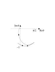
FIG. 8.: Dotted line: the trajectory of the retarded component of $\theta$ as a function of position for an infinite SN junction with coincident phases and $\epsilon/\Delta=0.6$ and $\gamma=0.1$. The trajectory starts at $x=0$ and approaches the origin as $x\to\infty$. Solid line: The same for an SNS system, with $L/\xi=5$, starting at $x=-L/2$ and ending at $x=L/2$. The trajectory reverses direction at the centre of the N region, $x=0$.

Fig. 9 shows the local DoS $\nu(x)=\nu_{n}{\rm Re}\cos\theta(x)$ (cf. Eq. (44)) obtained for a particular value of the material parameter $\gamma=\nu_{n}\sqrt{D_{n}}/(\nu_{s}\sqrt{D_{s}})$, where $D_{n,s}$ are the diffusion constants in the N,S-region. Note that the deeper one proceeds into the S-region, the more the DoS approaches the characteristic BCS-form. Due to the proximity effect, the structure of the subgap ($\epsilon<|\Delta|$) DoS in the N-region remains non-trivial. Only in the asymptotic limit $x\rightarrow-\infty$, the region of suppressed DoS shrinks to zero and ’normal’ behaviour is restored. More precisely, substantial alteration of the DoS induced by the proximity effect is restricted spatially to a region of several diffusion lengths from the interface into the normal metal, or several (dirty) superconducting coherence lengths into the superconductor.

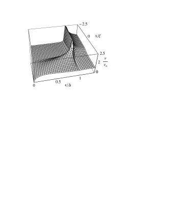
FIG. 9.: Local DoS of the infinite SN junction as a function of both energy and position for $\gamma=0.1$.

Fig. 10 shows how variation in $\gamma$ affects the DoS. In particular, we may take the ‘rigid’ limit $\gamma\rightarrow 0$, for which the bulk superconducting value of the Usadel angle is imposed at the interface, and retain a non-trivial structure in the spectrum.

FIG. 10.: The effect of $\gamma$ on the energy dependence of the DoS, at $x=1.5\xi$.

For a more comprehensive discussion of the local DoS of the system above we refer the reader to e.g. Ref.[70].

SNS-junction: As an example representative for the class of SN-systems with compact metallic region we next discuss the quasi one-dimensional SNS-junction displayed in fig. 2. As opposed to the SN-system, the physics of the SNS-system does depend on the phases of the order parameters in the superconducting terminals. For this reason SNS-systems with an in-built possibility to tune the phases of the superconductors are sometimes referred to as Andreev interferometers. In Appendix C 1 the quantitative solution of the Usadel equation is discussed explicitly for the comparatively simple case $\Delta\varphi\equiv\varphi_{1}-\varphi_{2}=0$.

An analytic solution to the general case, $\Delta\varphi\neq 0$, is also possible, although cumbersome. In the limits of a very short ($L\ll L_{\epsilon}$) and very long ($L\gg L_{\epsilon}$) junction, separate approximation schemes to the general solution may be employed: the short junction case has been treated by Kulik and Omelyanchuk [36] (for $L\ll\xi,L_{\epsilon}$) and Likharev [30, 32] (for $\xi\ll L\ll L_{\epsilon}$), while the long junction case ($L\gg\xi,L_{\epsilon}$) has been treated by Zaikin and Zarkov [31, 33]. At this point we restrict ourselves to a discussion of a few qualitative characteristics of the solutions obtained in various regimes.

The most conspicuous feature of the system is the appearance of a minigap, $E_{g}$. As mentioned in section II, the precise form of the gap depends on the phase difference $\Delta\varphi$. Its maximum width is taken for $\delta\varphi=0$, while this width tends to $\Delta$ and $E_{c}$ for short and long (as defined above) junctions, respectively. With growing phase difference, $E_{g}$ shrinks until, at $\Delta\varphi=\pi$, it closes altogether[35] (apart from a ’microgap’ of the width of the single particle level spacing[10] – the latter is induced by the general phenomenon of level repulsion in disordered metals).

We take as illustrative the case of an SNS-junction with coincident phases, and of arbitrary width. In this case, the solution for ${\mathbf{q}}$ again lies in the 1-3-plane and is parametrized, as before, by the angle $\cos\theta={\mathbf{q}}\cdot\hat{e}_{3}$. Fig. 8 shows the trajectory of the retarded $\theta$ in the complex plane as a function of position, and fig. 11 shows the local DoS as a function of both energy and position. Note, as compared to the infinite SN case (fig. 9), the appearance of the minigap, $E_{g}$, which is below the superconducting gap and independent of position.

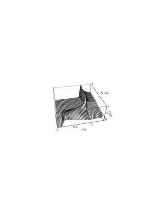
FIG. 11.: The local DoS for the SNS-junction as a function of both energy and position, for $L/\xi=5$, $\gamma=0.1$ and $\varphi=0$.

Figs. 12 and 13 show how variation of the material parameter $\gamma$ affects the local DoS. Further, fig. 13 shows how the local DoS at the SN-interface decreases as $\gamma$ is reduced (e.g. as the ratio of the disorder concentrations in the S- and the N-region is lowered.)

FIG. 12.: The effect of $\gamma$ on the energy dependence of the local DoS at the centre of the junction. Here $L/\xi=3$.

FIG. 13.: The effect of $\gamma$ on the position dependence of the DoS for the SNS-junction, with $\epsilon/\Delta=0.5$ and $L/\xi=3$.

VII Fluctuations

Having discussed the mean field content of the theory, we now turn to the central issue of this paper, that of mesoscopic fluctuations. The generality of the field theoretic machinery we have been discussing is such that it may be employed to analyse the majority of fluctuating observables in SN-systems. Our strategy of extending the conventional $\sigma$-model formalism allows us to take full advantage of the versatility of an approach that has been greatly developed in the study of fluctuation phenomena in purely N-mesoscopic systems. Yet in order not to diversify too much, we focus here on the discussion of the specific example of spectral fluctuations. In fact, the status of spectral fluctuations is slightly higher than that of an ordinary example, since a vast number of fluctuation phenomena are directly or indirectly related to fluctuations in the single particle spectrum (see Ref. [64, 88] for review).

A specific issue is the nature of fluctuations in the local DoS around the mean values (displayed in figs. 9 and 11). To characterize these fluctuations quantitatively, we employ the correlation function (22). Representing the correlation function in terms of Green functions (cf. Eq. (21)), we see that we need to compute functional expectation values of the type specified in Eq. (52). An evaluation of Eq. (52) on the mean field level discussed previously leads to a vanishing fluctuation component, $\langle{\cal G}^{\rm r}{\cal G}^{\rm a}\rangle-\langle{\cal G}^{\rm r}\rangle\langle{\cal G}^{\rm a}\rangle$, due to the fact that the mean field configuration, $\bar{Q}$, is diagonal in the ar-indices. In other words, there is no connection between advanced and retarded components and the functional evaluation of the product of Green functions equals the product of the averages. Consequently the physics of mesoscopic fluctuations is contained entirely in fluctuations around the block diagonal mean field configuration: $\bar{Q}\to T\bar{Q}T^{-1}$. At first sight the analysis of the fluctuation degrees of freedom, $T$ – after all a 16-dimensional matrix – seems to be a complicated task. Fortunately the totality of fluctuations may be organized into three separate types, each with its own physical significance. Such a classification scheme leads to a substantial simplification of the analysis. To be specific, we distinguish between fluctuation matrices, $T$, that

• are diagonal in the space of advanced and retarded components. These types of fluctuations still do not give rise to correlations between retarded and advanced Green functions. Nonetheless they are of physical significance: Quantum corrections to the Usadel solution are described by fluctuations of this type. We elaborate on these effects in section VII A.

• are non-diagonal in ar-space but are proportional to unity in ph-space, $[T,{\mathbf{\sigma}}^{\rm ph}]=0$. Fluctuations of this type do induce correlations between different Green functions and thereby mesoscopic fluctuations. They will be discussed in detail in section VII B.

• fulfill neither of the conditions a) and b). Whereas the physical significance of these fluctuations is less clearly identifiable than the one of the a- or b-type fluctuations, they are nevertheless of importance. The reason is that the c-type fluctuations tend to destroy at sufficiently high energies the correlations that derive from mesoscopic b-type fluctuations.

The three fluctuation types are summarized in the following table:

type	structure in ar space	ph space	lead to
a	diagonal	non-diagonal	corrections to Usadel Green function
b	non-diagonal	$\propto\openone^{\rm ph}$	mesoscopic fluctuations
c	non-diagonal	non-diagonal	destruction of b-type fluctuations

Besides the criteria a)–c), further restrictions to be imposed on the fluctuation matrices follow from two fundamental symmetries of the model: Firstly, general convergence criteria[64] enforce the condition

$$T^{\dagger}=\eta T^{-1}\eta^{-1},$$ (70)

where

$\displaystyle\eta=E_{11}^{\rm bf}\otimes\sigma_{3}^{\rm ph}\otimes\sigma_{3}^{\rm ar}+E_{22}^{\rm bf}.$

Secondly, the tr-space structure of the model implies[64]

$$T^{T}=\tau T^{-1}\tau^{-1},$$ (71)

where

$\displaystyle\tau=E_{22}^{\rm bf}\otimes i\sigma_{2}^{\rm tr}+E_{11}^{\rm bf}\otimes\sigma_{1}^{\rm tr}.$

For future reference we note that it is often convenient to represent both the matrices $T$ and the above symmetries in terms of the generators of the fluctuations:

$$T=\exp(W),$$ (72)

where the generators $W$ are subject to the constraints

$$W^{\dagger}=-\eta W\eta^{-1}$$ (73)

and

$$W^{T}=-\tau W\tau^{-1}.$$ (74)

The above scheme generally classifies the various types of fluctuation corrections to the quasiclassical picture of dirty superconductivity. Beginning with the a-modes, we now turn to a more comprehensive discussion of these fluctuations. Although we do not provide by any means a comprehensive survey of the full diversity of effects, we will find even in simple geometries of SNS-structures a significant range of fluctuation types and associated phenomena. In order to prevent the subdivision of these phenomena into excessively many classes, we assume throughout that the spatial extent of the N region is sufficiently large that $E_{c}\ll\Delta$. In this case, the minigap of the SNS-junction with zero phase difference, $\Delta\varphi=0$, lies at energy $E_{c}$. The significance of this restriction will be discussed further below, in section VIII.

A a-Type Fluctuations: Quantum Corrections to the Quasiclassical Theory

In this section, fluctuations of type a) around the Usadel saddle point will be considered. After specifying the general structure of these fluctuations, we will exemplify their effect by discussing the quantum corrections to the quasiclassical picture of single particle properties of SNS-structures. Other types of SN-structures can straightforwardly be subjected to an analogous analysis.

Fluctuations of type a) are diagonal in ar-space. Since the saddle point $\bar{Q}$ is also ar-diagonal, the full effect of the a-type fluctuations may be studied by considering just one of the ar-sectors of the model action (49). For example, we may consider the retarded sector describing the behaviour of a single, disorder-averaged retarded Green function. The restricted action is given by

$$S_{\rm ret}[Q^{11}]=-{\pi\nu_{n}\over 8}\int{\rm str}\left[D(\widetilde{\partial}Q^{11})^{2}+4iQ^{11}\left(i|\Delta|\sigma_{1}^{\rm ph}+\epsilon\sigma_{3}^{\rm ph}\right)\right],$$ (75)

where the eight dimensional matrix field $Q^{11}$ denotes the rr-block of $Q$ and the parameter $\omega$ (which is meaningless for a single Green function) has been dropped. To keep the notation simple, we will henceforth (until the end of the section) denote $Q^{11}$ again by $Q$.

Following the general philosophy of our classification, we organize the field $Q$ into a saddle point contribution $\bar{Q}$ (which is given by the solution of the retarded Usadel equation) and a-type fluctuations around it:

$$Q=RQ_{f}R^{-1},\qquad Q_{f}=T\sigma_{3}^{\rm ph}T^{-1},$$ (76)

where $R$ represents the inhomogeneous rotation parametrising the saddle-point,

$$\bar{Q}={\mathbf{q}}\cdot{\mathbf{\sigma}}^{\rm ph}=R\sigma_{3}^{\rm ph}R^{-1},$$ (77)

and the rotation matrices $T$ generate the a-fluctuations. More precisely, $T\in{\bf G}/{\bf H}$, where ${\bf G}$ is the group of eight dimensional matrices subject to the constraints (see Eq. (70)),

$$T^{\dagger}=\eta_{a}T^{-1}\eta_{a}^{-1},\qquad\eta_{a}=E_{11}^{\rm bf}\otimes\sigma_{3}^{\rm ph}+E_{22}^{\rm bf},$$ (78)

and Eq. (71). The subgroup ${\bf H}\subset{\bf G}$ is defined through ${\bf H}=\{h\in{\bf G}|[h,\sigma_{3}^{\rm ph}]=0\}$. Note that these symmetry relations imply that the matrices $T$ span Efetov’s eight dimensional coset space of orthogonal symmetry. In other words, save for the presence of the order parameter (and the different coupling of magnetic fields), the action (75) is identical to that of a conventional $\sigma$-model for an advanced and a retarded normal metal Green function.

In order to understand more fully the effect of the fluctuation matrices $T$, we first have to analyze their commutation behaviour with the different contributions to the action (75), i.e. the magnetic field, the energy term and the order parameter. Surprisingly, it turns out that there is a subset of $T$’s which not only commute through the order parameter (no matter what its phase) but also are insensitive to magnetic fields. For reasons that will become clear below, we will call these matrices the C-modes. In the limit $\epsilon\rightarrow 0$, the C-modes become completely massless. This implies that for low energies these modes need a special, or non-perturbative, treatment.

1 The C-Modes: Non-Perturbative Corrections to Quasiclassical Green Functions

Amongst the set of a-type matrices, $T$, consider the subset $T_{C}\equiv\exp(W_{C})$, subject to the additional constraints,

1. $[\sigma_{1}^{\rm ph},W_{C}]=0$ (order parameter $1$-component commutes through), and

2. $[\sigma_{3}^{\rm ph}\otimes\sigma_{3}^{\rm tr},W_{C}]=0$ (no coupling to magnetic field).

In combination with eqns. (73) and (74), this gives altogether four constraints and the non-trivial statement is that a set of generators $W_{C}$ obeying all of them actually exists. These are the C-modes. Before turning to the actual construction of these modes, let us qualitatively discuss some of their general properties.

First note that the conditions 1. and 2. above imply that the C-modes further commute with the 2-component of the order parameter. This follows from the observation that the phase twist needed to interpolate between the 1- and the 2-component of the order parameter is equivalent to the appearance of a magnetic gauge field which (see 2.) is invisible to the $W_{C}$’s. Being insensitive to both magnetic fields and order parameters with arbitrary phase positioning, the C-modes merely couple to the gradients and the energy term in the action (75). In the limit of small $\epsilon$, they become completely massless. More precisely, for a spatially constant $T_{C}^{0}\in{\bf G}_{C}$, where ${\bf G}_{C}$ is the subgroup of ${\bf G}$ fulfilling the extra constraints 1. and 2., $S[T_{C}^{0}\bar{Q}\left(T_{C}^{0}\right)^{-1}]\stackrel{{\scriptstyle\epsilon\rightarrow 0}}{{=}}S[\bar{Q}]$.

Physically, the C-modes represent modes of quantum interference in SN-systems which survive magnetic fields. Within a different formalism, these modes have for the first time been noticed in Ref. [17]. Subsequently various physical phenomena caused by their presence have been discussed in the literature:

• In the initial paper, Ref. [17] mentioned above, it was observed that in SN-systems weak localization corrections to the conductance may survive magnetic fields. The quantum interference process responsible for that effect is associated with the C-modes.

• In Ref. [10], an SN-system subject to a magnetic field, but not exhibiting a minigap (due to suppression of the proximity effect by the magnetic field), was considered. In this case the single-particle DoS vanishes at the chemical potential on a scale set by the mean level spacing. The existence of this ’micro-gap’ is also an effect caused by the C-modes.

• Feigl’man and Skvortsov[61] discuss the effect of C-modes on the transport behaviour of vortices in moderately clean type II-superconductors.

• The above phenomena relate to mean single particle properties. For the sake of completeness, we here mention some manifestations of C-mode fluctuations in two-particle properties: The level statistics of SN-quantum dots in a magnetic field falls into a symmetry class that is different from any of the standard Wigner-Dyson classes. Referring to a classification scheme due to Cartan, the SN/magnetic field symmetry class has been termed ’class C’[10]. As in standard mesosocopic systems, these level fluctuations can also be associated with channels of microscopic quantum interference. Whereas Wigner-Dyson fluctuations in diffusive N-systems are caused by ’diffuson’ and ’Cooperon’ modes, the class C fluctuations are connected to the modes specified above, and hence the name ’C-modes’. A $\sigma$-model formulation of the C-mode spectral statistics of random matrix ensembles was presented in Ref. [19].

  C-type level statistics in vortices has recently been microscopically derived by Skvortsov et al. [62]. Thermal transport carried by C-modes through the core of superconductor vortices is considered in a recent paper by Bundschuh et al. [63].

Being effective already on the level of single particle properties, the C-modes must originate from interference processes between particles and holes. However, they cannot be identical with the modes displayed in figure 1 (b), since the latter are field sensitive. A typical type-C path configuration is displayed in figure 14. In the analysis below we will derive quantitative expressions for processes of this type.

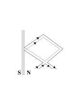
FIG. 14.: Semiclassical illustration of an interfering path configuration contributing to the C-mode corrections to the DoS. Compare the relative orientation of the arrows with those appearing in figure 1 (b).

After these general remarks, we next turn to the analysis of the C-mode contribution within the $\sigma$-model formalism. Specifically, we will discuss the effect of these modes on the mean density of states of the SNS-geometry displayed in figure 2.

Before turning to the core of the discussion, let us make a technical remark which will have some impact on the organization of the remainder of the section: The invariance of the action under spatially constant C-transformations , $S[T_{C}^{0}\bar{Q}\left(T_{C}^{0}\right)^{-1}]\stackrel{{\scriptstyle\epsilon\rightarrow 0}}{{=}}S[\bar{Q}]$ suggests an interpretation of these modes as a global symmetry of the action. In particular, it is more natural to let them act on $\bar{Q}$ from the outside: $Q=T_{C}\bar{Q}T_{C}^{-1}$ (compare with the inside representation of general a-fluctuations, Eq. (76), and the footnote on p.78). Of course it is possible to forcefully contrive an inside parameterization for the C-fluctuations, via $T_{C}\bar{Q}T_{C}^{-1}=R\tilde{T}_{C}\sigma_{3}\tilde{T}_{C}^{-1}R^{-1}$, where the unitarily transformed $\tilde{T}=R^{-1}T_{C}R$. In practice, however, this representation is inconvenient and, more seriously, makes it difficult to separate the C-mode fluctuations from general fluctuations around the saddle point. These considerations imply that, in general, it is difficult to treat the C-modes and the rest of the a-type fluctuations simultaneously. Physically, however, these problems are of little significance: Below it will be shown that the minimum price in energy associated with a non-C-fluctuation is of ${\cal O}(E_{c})$. This implies that two regimes with qualitatively different fluctuation behaviour exist:

• Low energies, $\epsilon\ll E_{c}$, where the C-modes are relevant, whereas the other a-fluctuations can safely be ignored, and

• High energies $\epsilon>E_{c}$, where all fluctuations have a comparable action of ${\cal O}(E_{c})$ and it is pointless to carefully distinguish between the different types (C or other).

Below we will discuss these cases separately. Although our analysis is not applicable to the crossover regime of intermediate energies, we do not expect qualitatively remarkable phenomena to arise there.

Low energies, $\epsilon\ll E_{c}$: To quantitatively analyse the fluctuation physics in this regime, we need first to derive an effective action for the C-modes. Fluctuations other than C are ignored.

To this end, we use that $[T_{C},\sigma_{1}^{\rm ph}]=[T_{C},\sigma_{2}^{\rm ph}]=0$ and represent the $Q$-field as

$$Q=q_{3}Q_{C},\qquad Q_{C}=T^{\vphantom{-1}}_{C}\sigma_{3}^{\rm ph}T_{C}^{-1}.$$ (79)

Substituting this parameterization into Eq. (75), we obtain the desired action

$$S_{C}[Q_{C}]=-{\pi\nu_{n}\over 8}\int{\;\rm str\;}\left[Dq_{3}^{2}(\partial Q_{C})^{2}+4iq_{3}\epsilon Q_{C}\sigma_{3}^{\rm ph}\right].$$ (80)

Among the general set of C-type fields $Q_{C}$ , there is a particular mode $Q_{C}^{0}=T^{0\vphantom{-1}}_{C}\sigma_{3}^{\rm ph}(T^{0}_{C})^{-1}$ which not only has C-symmetries but also is spatially constant. Substituting this ’zero-mode’ into (80), we obtain the action

$$S_{C}^{0}[Q_{C}^{0}]=-{i\tilde{s}\over 2}{\;\rm str\;}\left[Q_{C}^{0}\sigma_{3}^{\rm ph}\right],$$ (81)

where

$$\tilde{s}=\pi\epsilon\nu_{n}\int q_{3}.$$ (82)

Note that deep in N, where $q_{3}=1$, $\tilde{s}$ = $\pi\epsilon/\bar{d}$, where $\bar{d}$ is the mean level spacing, coincides with the standard parameter $s$ [64] commonly employed in the literature on spectral correlations in metals.

In order to give the above zero mode action some physical significance, it has to be shown that it is energetically gapped against the action of the higher (spatially fluctuating) field configurations of C-symmetry. The spectrum of fluctuating C-modes can be determined at various levels of accuracy. For our purposes, it suffices a) to demonstrate that a ground state gap exists and b) to coarsely estimate its magnitude. To do so, we first note that the mode spectrum is essentially determined by the gradient operator appearing in Eq. (80). Integrating by parts, the latter can be rewritten as

$$\sim\int q_{3}^{2}{\;\rm str\;}\left[QDq_{3}^{-2}\partial(q_{3}^{2}\partial)Q\right].$$ (83)

The rationale behind this reformulation is that $Dq_{3}^{-2}\partial(q_{3}^{2}\partial)$ may be regarded as a differential operator which is Hermitian with respect to the scalar product $\langle f,g\rangle\equiv\int q_{3}^{2}fg$. Being Hermitian with compact support (taking $q_{3}\rightarrow 0$ in S), the spectrum of the differential operator is discrete. To estimate the spacing $\Delta E$ between the zero eigenvalue of the spatially constant eigenmode and the first excited eigenvalue, we use the fact that the range of support of the operator is set by $L$, the extension of N. Standard reasoning for the eigenvalue structure of one-dimensional Hermitian differential operators with compact support then leads to the estimate $\Delta E\sim D/L^{2}=E_{c}$. Notice that the actual spatial structure of the excited eigenfunctions may be complicated. For example, unlike with standard applications of $\sigma$-models to N-systems, typical eigenmodes of the action obey neither Neumann nor Dirichlet boundary conditions, but rather exhibit more complicated edge behaviour which, in principle, may be derived from Eq. (83) once $q_{3}$ is known. For our purposes, entering this discussion will turn out to be unnecessary.

The considerations above show that for energies $\epsilon\ll E_{c}$, the action is governed by the spatially constant C-mode. It is reasonable to ask for which physical applications such low energies may be expected to play a rôle. For zero phase difference between the superconductor terminals, the minigap is of ${\cal O}(E_{c})$ and, with regard to the DoS, the C-mode fluctuations are expected to be of little importance. To actually make visible the impact of these fluctuations on the DoS, we concentrate here on the case of a junction close to $\pi$-phase difference, i.e. a junction where the gap is nearly but not completely closed: $E_{g}\ll E_{c}$. Note that previous studies of the C-type fluctuations having concentrated on the limiting case where the proximity effect is totally suppressed ($E_{g}\to 0$). It is worth remarking that, while we have limited here our comments to issues surrounding the DoS, subgap properties of SNS-junctions, such as the Josephson coupling, may well be affected by the C-fluctuations, even under the broader conditions of a fully-established proximity effect. However, the analysis of these phenomena lies beyond the scope of this paper.

Focusing on the range of applicability of the action (81), we notice that for very small energy parameters, so that $\tilde{s}={\cal O}(1)$, the zero mode must be treated in a non-perturbative manner. Very much as in the study of N $\sigma$-models at low energy scales, the fluctuations become unbounded as $\tilde{s}\rightarrow 0$. Rather than perturbatively expanding in terms of the generators $W_{C}$, it then becomes necessary to integrate over the entire manifold of matrices $T_{C}$. Non-perturbative analyses of this type have previously been applied to the study of a random matrix ensemble[19] of non-proximity effect SN-structures and of normal core excitations of vortices in superconductors [62]. Here we discuss how the C-fluctuations affect the low energy behaviour of the Gorkov Green function in SNS-junctions.

To this end, we first need to specify a global parameterization of the matrices $T_{C}$. It is a straightforward (if lengthy) matter to show that a general $8\times 8$-matrix $T_{C}=\exp(W_{C})$, subject to both the general constraints (73) and (74) and 1. and 2., can be parameterized as

$$T_{C}=vua,$$ (84)

$$\qquad a=\exp\left(\frac{i\theta}{2}E_{22}^{\rm bf}\otimes\sigma_{1}^{\rm ph}\otimes\sigma_{1}^{\rm tr}\right),$$ (85)

$$\qquad u=\exp\left(iyE_{22}^{\rm bf}\otimes\sigma_{3}^{\rm tr}\right)\otimes\openone_{\rm ph},$$ (86)

$$\qquad v=\exp\left(\begin{array}[]{cc}&\lambda-\mu\sigma_{3}^{\rm tr}\\ \mu+\lambda\sigma_{3}^{\rm tr}&\end{array}\right)_{\rm bf}\otimes\openone_{\rm ph},$$ (89)

Where $\lambda$ and $\mu$ are Grassmann variables. For the (invariant) measure associated to the integration over the matrix $Q_{C}$ we obtain (cf. the analogous but more difficult calculations of integration measures in [64])

$\displaystyle\int dQ_{C}(\dots)=\int_{0}^{2\pi}\frac{dy}{2\pi}\int_{0}^{\pi}\frac{d\theta\sin\theta}{2\sin^{2}(\theta/2)}\int d\lambda d\mu(\dots).$

Substituting the parametrisation (84) into the action (81) we obtain

$$S_{C}^{0}[Q_{C}^{0}]=-2i\tilde{s}(\cos\theta-1).$$ (90)

As an example, we apply this action to a calculation of the C-mode corrections to the local DoS. Substituting the zero mode integration over $Q_{C}$ for the functional expectation value in Eq. (44) and performing the (trivial) integrations over Grassmann variables and $y$, we obtain

$$\nu=\nu_{n}{\,\rm Re\,}\left\{q_{3}\left(1-\frac{1}{2}\int_{0}^{\pi}d\theta\sin\theta e^{2i\tilde{s}(\cos\theta-1)}\right)\right\}$$

$$\hskip 14.22636pt=\nu_{n}{\,\rm Re\,}\left\{q_{3}\left(1-\frac{1-e^{-4i\tilde{s}}}{4i\tilde{s}}\right)\right\}$$

$$\hskip 14.22636pt=\nu_{n}{\,\rm Re\,}\left\{q_{3}\left(1-\frac{\sin(4\tilde{s})}{4\tilde{s}}+\frac{1-\cos(4\tilde{s})}{4i\tilde{s}}\right)\right\}.$$

The last line tells us that for small energies, $\tilde{s}\rightarrow 0$, the DoS always (i.e. including the case of a $\pi$-junction) vanishes on a scale set by the mean level spacing. This is the DoS ’micro-gap’ that has been discussed previously in Refs.[10, 19, 61, 62]. Moreover, for general $\tilde{s}$, possessing real and imaginary components, the DoS is not only determined by ${\rm Re\;}q_{3}$ but also by the imaginary component, ${\rm Im\;}q_{3}$, of the Usadel solution. Finally, $\tilde{s}$ contains the Usadel solution in an integrated form, that is, the C mode introduces some non-local influence on the local DoS by the Usadel solution at different points of the system. The corrections vanish algebraically as $\tilde{s}^{-1}$. For ${\rm Im\;}\tilde{s}>1$ the (oscillatory) factors containing the exponentiated parameter $\tilde{s}$ can be neglected and we obtain the simplified result

$$\nu\simeq\nu_{n}\left({\rm Re\;}q_{3}+\frac{1}{4}{\;\rm Im\;}\frac{q_{3}}{\tilde{s}}\right).$$ (91)

Note that the definition (82) implies that for the global DoS ($\sim\int\nu$) the algebraic corrections vanish. For a diagrammatic interpretation of this correction to the Usadel DoS, cf. Ref. [10].

For $\Delta\varphi=\pi-0.0025$ and $g=5$, the quasiclassical DoS and the corrections to it are displayed in figure 15. We display here the DoS in the vicinity of the minigap, at an energy regime similar to that considered by Zhou et al. [71]. For this set of parameters, the quasiclassical DoS displays a very strong peak, which dies down for $(\epsilon-E_{g})/E_{g}={\cal O}(1)$.

$\displaystyle\begin{array}[]{ccc}\psfig{height=142.26378pt}&&\psfig{height=142.26378pt}\\ {\em(a)}&&{\em(b)}\end{array}$

FIG. 15.: (a) Quasiclassical DoS and (b) the C-mode correction for $\Delta\varphi=\pi-0.0025$ and $g=5$, at the centre of the junction and in the vicinity of the minigap. The dotted line represents the non-oscillatory part of the correction, as given by Eq. (91).

Large energies, $\epsilon>E_{c}$: For large energies, the isolated 0-mode action is no longer of significance. The energy of all modes, C- or other, is larger than $E_{c}$. In particular, spatially fluctuating configurations (with a ’kinetic’ energy cost of ${\cal O}(D/L^{2}=E_{c})$) need to be taken into account, too. Since the energy associated with all these fluctuations is parametrically of the same order, separating the C-modes from the rest becomes pointless. In the next section we discuss the corrections to quasiclassics at energies larger or comparable to $E_{c}$ arising from a perturbative treatment of all a-type fluctuations.

2 Perturbative Corrections to the Quasiclassical Green Function

In the following we consider the impact of a-type fluctuations on the ’high’ energy ($\epsilon\sim E_{c}$) behaviour of the average Gorkov Green function. To keep our discussion simple, we limit consideration in this section to a SNS geometry where time-reversal symmetry is maintained (i.e. where the phase difference between the two superconductors, $\Delta\varphi$, is zero.) The violation of time-reversal symmetry through the variation of the phase of the order parameter across the junction will not change our discussion qualitatively.

Specifically, the questions we are going to address are

• Do quantum corrections lead to the suppression of the minigap in the normal region?

• If so, does the minigap edge remain sharp, or are states introduced at all energy scales below the gap?

As in the previous sections, the theory developed in this section may also be straightforwardly generalized to other types of geometries and observables.

For large energies $\epsilon\sim E_{c}$, it is convenient to parameterize the totality of a-type fluctuations as in Eq. (76). Due to the comparatively large energy cost associated with fluctuations around the Usadel saddle point, it is sufficient to expand the action to low orders in terms of the generators $W$ of the fluctuation matrices $T$. Substituting the parameterization (76) into the action (75), we obtain

$$S[Q]=-{\pi\nu_{n}\over 8}\int{\rm str}\left[D(\widetilde{\partial}Q_{f})^{2}+4i\epsilon R^{-1}\sigma_{3}^{\rm ph}RQ_{f}\right],$$ (92)

where $\widetilde{\partial}=\partial+[R^{-1}\partial R,\;]$. Note that the above action does not contain the superconducting order parameter. This is accomplished by demanding that the non-C-type fluctuations obey Dirichlet boundary conditions at the NS-interface. As a consequence these modes are spatially varying with a minimum fluctuation energy of ${\cal O}(E_{c})$, which justifies their perturbative treatment. As for the C-modes, these do not couple to the order-parameter anyway. In principle, their treatment is difficult because, as mentioned above, they a) fulfill mixed boundary conditions different from Dirichlet or Neumann and b) are difficult to separate from the complementary set of a-type fluctuations. However, for large energies we believe these complications to be physically irrelevant: The spectrum of all fluctuating modes is discrete with a typical spacing of ${\cal O}(E_{c})$. For energies $\epsilon$ comparable with $E_{c}$, all modes need to be summed over. Under these conditions, the detailed structure of boundary conditions and/or eigenvalues of individual modes becomes largely inessential; What matter are the global features of the energy spectrum associated with the fluctuations, most importantly, the typical mean energy spacing. For this reason, we feel justified in ignoring the different boundary behaviour of the C-modes and to globally impose Dirichlet boundary conditions (thereby correctly modelling the typical spacing between consecutive eigenmodes). We believe that this simplification does not lead to qualitative errors.

To obtain the perturbative expansion of the action, we employ the exponential parameterization $T=\exp(W)$ and expand the generators $W$ in terms of ph-Pauli matrices, $W=w_{1}\sigma_{1}^{\rm ph}+w_{2}\sigma_{2}^{\rm ph}$ (so that $[W,\sigma_{3}^{\rm ph}]_{+}=0$). For zero phase difference, the Usadel solution encoded in the rotation matrices $R$ can be parameterized in terms of a single angle $\theta$ (cf. Eq. (C1)). The rotation matrices $R$ mediating between $\sigma_{3}^{\rm ph}$ and the Usadel saddle point then take the simple form

$$R=\exp\left[-i\frac{\theta}{2}\sigma_{2}^{\rm ph}\right],\qquad(\partial R)R^{-1}=-{i\over 2}\sigma_{2}^{\rm ph}\partial\theta.$$ (93)

Substituting these expressions into the action and expanding up to second order in $w_{i}$, it is a straightforward matter to show that

$$S[W]=\pi\nu_{n}\int{\rm str}_{0}\left[D\left((\partial w_{1})^{2}+(\partial w_{2})^{2}-(\partial\theta)^{2}w_{1}^{2}\right)-2i\epsilon\cos\theta\left(w_{1}^{2}+w_{2}^{2}\right)\right]+O(W^{3}).$$ (94)

Here and in the following, the notation ’${\rm str}_{0}$’ represents a supertrace over all degrees of freedom except for the ph-components, which have been traced over. The absence of terms at first order in $W$ is assured by the expansion around the saddle-point configuration of $Q$.

To eliminate the term in $\sim(\partial\theta)^{2}$, we make use of the fact that the Usadel equation (C2) possesses the first integral,

$$D(\partial\theta)^{2}-4i\epsilon(\cos\theta-\cos\theta(0))=0,$$ (95)

where we have used the fact that in the middle of the junction, $\partial\theta=0$. Substituting this result into Eq. (94), we obtain

$$S[W]=\pi\nu_{n}\int{\rm str}_{0}\left[D\left((\partial w_{1})^{2}+(\partial w_{2})^{2}\right)+2i\epsilon w_{1}^{2}(2\cos\theta(0)-3\cos\theta)-2i\epsilon w_{2}^{2}\cos\theta\right].$$ (96)

To compute corrections to the DoS, we substitute the exponential parameterization into the functional representation (44) to find

$$\nu(x) = {\nu_{n}\over 8}{\rm Re}\left\langle{\rm str}\left(R\sigma_{3}^{\rm bf}\otimes\sigma_{3}^{\rm ph}R^{-1}Q\right)\right\rangle_{Q}$$ (97)

$$= \nu_{n}{\rm Re}\cos\theta\left[1+\frac{1}{2}\left\langle{\rm str}_{0}\left(\sigma_{3}^{\rm bf}(w_{1}^{2}+w_{2}^{2})\right)\right\rangle_{W}\right]$$ (98)

$$= \nu_{n}{\rm Re}\cos\theta\left[1+\frac{1}{\pi\nu_{n}L_{\perp}^{d-1}}\left(\Pi_{1}(x,x)-\Pi_{2}(x,x)\right)\right],$$ (99)

where $x$ is the coordinate along the junction and $L_{\perp}$ is spatial extent of the N region in all other directions. The last line in Eq. (97) is obtained by an application of Wick’s theorem[64] to the Gaussian expectation values $\langle\sigma_{3}^{\rm bf}w_{i}^{2}\rangle_{W}$. The ’propagators’ $\Pi_{i}$ play the rôle of generalized diffusion poles. They are defined through

$$\left[-D\partial_{x}^{2}+2i\epsilon(2\cos\theta(0)-3\cos\theta(x))\right]\Pi_{1}(x,y) = \delta(x-y),$$ (100)

$$\left[-D\partial_{x}^{2}-2i\epsilon\cos\theta(x)\right]\Pi_{2}(x,y) = \delta(x-y).$$ (101)

Without going into details we remark that the relative minus sign between $\Pi_{1}$ and $\Pi_{2}$ in (97) derives from the different symmetries of the matrices $w_{1}$ and $w_{2}$ under matrix transposition (cf. Eq. (74)).

We will not proceed any further analytically. In order to quantitatively evaluate the $\Pi$-dependent corrections to the DoS, one would have to compute the generalized diffusion poles (100). Due to the presence of the spatially varying terms $\sim\cos\theta$, a general solution of the differential equations is difficult. Nonetheless, quite a few characteristic properties of the DoS corrections can be deduced from (97) simply by inspection:

For asymptotically large energies $\epsilon\gg E_{c}$, one expects no influence of the superconductor on the normal metal. Indeed, in that limit, $\cos\theta\to 1$ implying that a) the Usadel DoS becomes metallic and b) $\Pi_{1}-\Pi_{2}\to 0$, i.e. no quantum corrections to the DoS.

For intermediate energies just above the minigap edge $E_{g}$, $\cos\theta$ varies smoothly as a function of position. In this regime Eq. (97) gives corrections of ${\cal O}(g^{-1})$ to the DoS whose quantitative evaluation is difficult.

Finally, let us consider subgap energies, $\epsilon<E_{g}$ (remaining of course outside the regime $\epsilon\ll E_{c}$). Here, according to the quasiclassical analysis, the DoS vanishes, implying that $\cos\theta$ is purely imaginary and the effective action (96) purely real. As a consequence, the propagators $\Pi_{i}$ are real, too, and the DoS, as computed according to (97), vanishes identically below the quasiclassical minigap edge. In other words, the perturbative inclusion of first order quantum corrections does not give rise to the appearance of states below the quasiclassical edge. The vanishing of ${\rm Re\,}(\cos\theta)$ actually suffices to demonstrate that the robustness of the gap pertains to all orders of perturbation theory.

This conclusion presents something of a puzzle: Taking into account quantum corrections, the above result indicates that the minigap remains fixed at energy $E_{g}$. The latter is determined by the bare value of the diffusion constant, $D=v_{F}l/d$. However, the intuition afforded by the one-parameter scaling theory of localization [74] suggests that observables such as the tunneling DoS should depend only on the value of $D$ renormalized by weak localization corrections. In bulk normal metallic samples, weak localization corrections (to two-particle properties) stem from mechanisms of quantum interference between trajectories connected through a time reversal operation. (see fig. 16(a)). In the present case, weak localization effects can arise due to the interference of particles and holes (see fig. 16(b)). Since holes bear similarity with time reversed particles, there is no conceptual difference to the above N-interference mechanism, and one expects a standard renormalization of the diffusion constant (albeit already on the level of one-particle properties). Yet, according to the analysis above, the minigap edge, a function of the unrenormalized $D$, is robust against perturbative quantum corrections in the particle/hole channel.

$\displaystyle\begin{array}[]{ccc}\psfig{height=142.26378pt}&&\psfig{height=142.26378pt}\\ {\em(a)}&&{\em(b)}\end{array}$

FIG. 16.: Renormalisation of the diffusion constant, $D$, by interference of (a) trajectories with their time-reversed counterparts, and (b) particles and holes.

In fact, the absence of weak localization corrections to the minigap edge signals the failure of the perturbation theory. To properly identify quantum weak localization corrections to the diffusion constant, and therefore the minigap edge, it is necessary to renormalize the saddle-point equation itself. This situation parallels that encountered in the study of the renormalization of the gap in a dirty bulk superconductor where quantum corrections (in the Cooper channel) lead to a renormalization of the gap equation (see e.g. Ref. [77]). In the present case, weak localization corrections to the minigap edge are obtained within a renormalization group procedure. Since, operationally, this procedure is somewhat technical, its description has been made the subject of appendix E.

The renormalization group procedure described in appendix E may be employed safely down to energy scales in excess of $E_{c}$. However, at energy scales in the vicinity of the minigap, the Cooperon propagator depends sensitively on the geometry and it becomes necessary to include the additional flow in $R$ (the matrix rotating to the RG-affected saddle point of the theory), coupled to that in $D$, as the cutoff is lowered towards $E_{g}$. Although the manner in which such renormalisation processes are included self-consistently lies beyond the scope of this paper, the outcome of the RG procedure can be summarized as follows: Treating quantum interference correction within a RG-scheme leads to a shift of the minigap edge. The overall structure of the gap edge (e.g.the non-analytic behaviour of the DoS in the vicinity of the DoS) is maintained. In particular, no states are found below the (renormalized) gap edge.

These findings leave us with the question whether indeed, no states exist below the (renormalized) gap edge or whether the computation simply has not been accurate enough. Although a quantitative analysis of this question is beyond the scope of this paper, we believe that the second option is the correct one: To find states below the minigap, one must account for contributions to the action which cannot be accessed by a perturbative shift of the inhomogeneous saddle-point. Contributions of this kind have been identified in bulk normal conductors as soliton-like configurations of the $Q$-matrix fields, and have been associated with a rare class of states which are described as “anomalously” or “nearly” localized within the metallic phase [80, 82, 83]. Poorly contacted to the superconductor, these states are able to exist at energies below the minigap and generate contributions to the average DoS exponentially small in $g$. Although we see the SN system as a useful and challenging arena in which to investigate the localization properties of such rare states, their consideration lies beyond the scope of this paper.

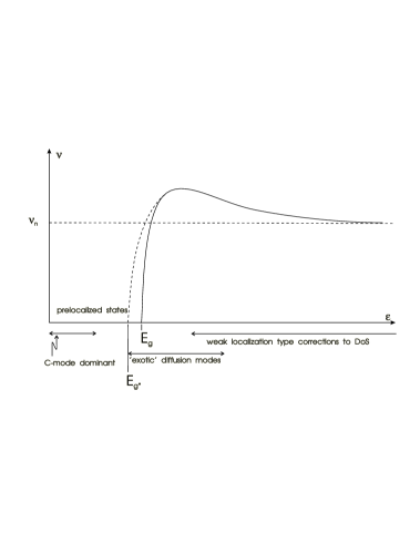
FIG. 17.: Schematic indication of the rôle of the various DoS corrections. $E_{g^{\ast}}$ denotes the renormalized gap edge.

Before leaving this section, let us in summary list the – admittedly diverse – set of a-type fluctuation mechanisms renormalizing the single-particle properties of mesoscopic SN-structures (see figure 17):

• For energies $\epsilon\gg E_{c}$, the N-component behaviour is largely metallic. However, the presence of the superconductor is exerted in terms of massive quantum corrections to the DoS and other single particle properties. The larger $\epsilon$ is, the smaller are the corrections.

• Energies just above the minigap edge $E_{g}$ are the most difficult to analyse. Quantum corrections to quasiclassics are carried by diffusion type modes which – due to the pronounced energetic and spatial inhomogeneity of the DoS – are difficult to treat analytically. By perturbatively including such corrections, one obtains corrections to the DoS above the gap. Both the position of the gap and the vanishing of the subgap density of states remain unchanged.

• By embedding the diffusive modes into an iteration of RG-analyses and solutions of renormalized Usadel-type mean field equations, one arrives at a shifted minigap edge. The non-analyticity of the gap is maintained – that is, there are no smooth DoS ’tails’ leaking downwards out of the sharp edge.

• Presumably, ’nearly localized’ subgap states can be found with a probability that is exponentially small in the metallic conductance $g$.

• Eventually, for energies $\epsilon\ll E_{c}$, the fluctuation physics is governed by the C-mode whose impact on various physical observables (for non-proximity effect SN-structures) has already been discussed in the literature.

It is important to question whether the above corrections can be made experimentally visible. As far as the DoS is concerned, the answer must be a conservative one: the chances are that it will be impossible to separate the high energy $1/g$-corrections from the Usadel background. Furthermore, for good metals ($g\gg 1$), finding nearly localized subgap states will also be difficult, since, as shown in Refs. [80, 82, 83], disorder configurations leading to nearly localized states are exponentially rare. Thus, as far as the mean DoS is concerned, the above fluctuation contributions will probably be hard to detect. However, the primary purpose of this section has been to demonstrate that a variety of interference mechanisms adding to the standard quasiclassical picture exist in principle. If and to what extent these fluctuations give rise to observable changes in single particle properties other than the DoS (e.g. the Josephson coupling characteristics) represents a subject of future research.

We now leave the issue of the renormalization of single particle properties and turn to the discussion of correlations between more than one Green function, as described by the b- and c-type fluctuations.

B b-Type Fluctuations: The Goldstone Mode

In this section we discuss the class of fluctuations around the Usadel saddle point which above has been denoted by ’type b)’. Unlike the a-fluctuations, fluctuations of type b) induce correlations between different Green functions. What makes the b-fluctuations particularly important is their Goldstone mode character: In the limit of vanishing energy difference between the considered Green functions, these modes become truly massless, a signature for the presence of pronounced mesoscopic fluctuations.

Consider the action (49) in the simple case $\omega_{+}={\mathbf{A}}=0$. Obviously, any transformation $\bar{Q}\rightarrow T_{0}\bar{Q}T_{0}^{-1}$ leaves the action invariant provided that $[T,\sigma_{i}^{\rm ph}]=0$. Among the group of matrices ${\bf G_{0}}\equiv\{T=T_{0}\otimes\openone^{\rm ph}\}$, there is a subgroup ${\bf H_{0}}\subset{\bf G_{0}}$, $[{\bf H_{0}},\sigma_{3}^{\rm ar}]=0$ which not only leaves the action invariant, but also the saddle point solution $\bar{Q}$ itself. As a consequence, fluctuation matrices contained in the subgroup ${\bf H_{0}}$ are completely ineffective and do not couple to the theory. However, the elements $T_{0}$ of the coset space ${\bf G_{0}}/{\bf H_{0}}$ do generate non-trivial transformations of the diagonal saddle point. Moreover, in the limit $T_{0}={\rm const.}$, these transformations do not alter the action – they are Goldstone modes.

Being Goldstone modes, the effective action of the $T_{0}$’s can only contain gradient terms and mass terms induced by sources of symmetry breaking, such as finite $\omega_{+}$ and ${\mathbf{A}}$. The actual structure of the action depends crucially on its behaviour under time reversal. For the sake of simplicity, we focus here on the two pure symmetry cases:

• Orthogonal symmetry: The action is time reversal invariant, ${\mathbf{A}}=0$.

• Unitary symmetry: Time reversal invariance is broken, $|{\mathbf{A}}|L\Phi_{0}^{-1}\gg g^{-1/2}$.

Here, $\Phi_{0}$ is the flux quantum. Note that ${\mathbf{A}}$ denotes the vector potential with account for the phase difference between the superconducting terminals, so that phase differences $\Delta\varphi\Phi_{0}^{-1}\gg g^{-1/2}$ suffice to drive the system into the unitary symmetry class. The reason that $g^{-1/2}$ appears as a measure for the strength of the perturbation is that, for $|{\mathbf{A}}|L\Phi_{0}^{-1}\gg g^{-1/2}$, the dimensionless coupling constant of the symmetry breaking operator in the action exceeds unity (see Appendix D). Alternatively, one may say that under these conditions, the mass of the ’Cooperon’ greatly exceeds the level spacing.

The derivation of the effective action, $S_{0}$, of the Goldstone modes is somewhat technical and has been deferred to Appendix D. Here we merely state the result,

$$S_{0}[Q_{0}]=-c_{\rm sym}\frac{\pi}{4}\int\left[\nu_{n}\tilde{D}{\,\rm str}_{0}\left(\partial Q_{0}\partial Q_{0}\right)+2i\omega_{+}\nu{\,\rm str}_{0}\left(Q_{0}\sigma_{3}^{\rm ar}\right)\right],$$ (102)

where $\tilde{D}=\frac{D}{2}(1-{\mathbf{q}}_{+}\cdot{\mathbf{q}}_{-})$ plays the rôle of a space dependent diffusion coefficient. The variation of $\tilde{D}$ with both position and energy is shown in fig. 18 for an SN junction with a typical choice of material parameter. In addition, $\nu$ is the space dependent, local DoS, as displayed already in fig. 9. (Notice that in the bulk of S both the diffusion constant and $\nu$ vanish. Hence, the support of the action of $Q_{0}$ is restricted to the N region.)

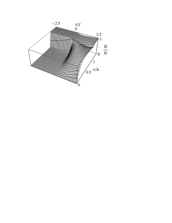
FIG. 18.: The effective diffusion constant, $\tilde{D}$, for the Goldstone modes in an SN junction as a function of both energy and position, for $\gamma=0.1$.

Further, in the case of

• Orthogonal symmetry: $c_{\rm sym}=1$, the matrices $T_{0}$ are eight dimensional and obey the time reversal symmetry relation (71), and of

• Unitary symmetry: $c_{\rm sym}=2$, the matrices $T_{0}$ are four dimensional (i.e. they do not carry a tr-index structure) and Eq. (71) is meaningless.

In either case the matrices $T_{0}$ obey the restricted version of the symmetry relation (70)

$$T_{0}^{\dagger}=\eta_{0}T_{0}^{-1}\eta_{0}^{-1},$$ (103)

where

$\displaystyle\eta_{0}=E_{11}^{\rm bf}\otimes\sigma_{3}^{\rm ar}+E_{22}^{\rm bf}.$

In summary, we see that the symmetry of the Goldstone fields is identical to those of the standard Efetov $Q$-matrix manifolds[64]. In other words, by freezing out the ph-degrees of freedom, the large 16-dimensional $\sigma$-model manifold collapses to smaller ones of dimensionality 8 (4) which are symmetrically identical to those encountered in orthogonal (unitary) applications of the standard $\sigma$-model.

Besides the general symmetry relations, a further condition to be imposed on the fields is that they obey Neumann boundary conditions $\partial_{\perp}T_{0}(x)=0$ at all SN-interfaces. The derivation of these boundary conditions is discussed in Appendix D.

So far the discussion has been for a general SN geometry. In order to actually demonstrate how the b-modes generate mesoscopic fluctuations we next consider a specific example, namely, the problem of DoS fluctuations above the minigap edge in an SNS-structure.

1 Level-Statistics in SNS-structures

It is well known that the single particle spectrum of mesoscopic, purely normal systems is governed by various types mesoscopic fluctuations (see e.g. Ref. [64] for review). The fluctuation behaviour can be characterized conveniently in terms of correlations $\sim\langle\nu(\epsilon-\omega/2)\nu(\epsilon+\omega/2)\rangle$ between the DoS’s at different energies. Extensive analyses of correlation functions of this type have shown that the DoS-correlations become increasingly universal in character, the lower the energy separation $\omega$ (a fact that follows heuristically from the interpretation of $\omega$ as an inverse time scale). In particular, for energies $\epsilon<E_{c}$ the correlations become fully universal in the sense that they depend on nothing more than the mean (and constant) level spacing $\bar{d}$ and the fundamental symmetries of the system. This is the regime of Wigner-Dyson statistics. For larger energies, the Wigner-Dyson behaviour crosses over to other and less universal types of statistics. Nevertheless, the correlations remain energetically long-ranged in the sense that they decay algebraically as a function of $\omega$.

Here we ask to which extend this behaviour carries over to the fluctuation behaviour of the SNS DoS in the vicinity of the minigap. As compared to normal metals, the situation is more intricate in that already the mean DoS is affected by mechanisms of quantum coherence. A conceivable situation is that the (strong) modes of quantum interference, giving rise to the particular structure in the mean DoS, decouple entirely from the modes responsible for DoS fluctuations. Another possibility is that one might end up with some kind of inseparable conglomerate of modes of interference, and thereby fundamentally non-universal types of spectral statistics. Here we demonstrate that the true picture lies somewhere halfway between these two extreme options: It is still possible to identify a regime of universal Wigner-Dyson statistics, albeit superimposed on an energetically non-uniform DoS. However, its range of validity shrinks down to a small energy window beyond which the correlations do become entirely non-universal.

To obtain specific information about spectral fluctuations in an SNS-structure, we apply the action (102) to the analysis of the SNS geometry, shown in fig. 2. The set of field configurations obeying Neumann boundary conditions at the SN-interfaces obviously contains a subset with trivial spatial dependence, $T_{0}={\rm const.}$ – the ’zero mode’. The zero mode action reads:

$$S_{0}[Q_{0}={\rm const.}]=-i\frac{\pi}{2}\frac{\omega_{+}}{\bar{d}(\epsilon)}{\rm str}_{0}[Q_{0}\sigma_{3}^{\rm ar}].$$ (104)

Here $\bar{d}(\epsilon)=(\int\nu(\epsilon))^{-1}$ denotes the average level spacing, which, in contrast to the purely normal case, is now energy dependent. Note the similarity with the action, (81), of the C-zero mode. The difference is in the pre-factor and in the physical spaces in which the matrices $Q$ and $Q_{C}^{0}$, respectively, operate.

In order to demonstrate any significance of the isolated zero mode action, we have to show that it is separated by an energy gap from the action of all other field configurations. At this point, the boundary conditions begin to play a crucial role. Expanding the fields in terms of cosines, that is, a complete set of functions compatible with Neumann boundary conditions, we see that, next to the zero mode, the field with least curvature varies as $\sim\rm cos(2\pi x/L)$. Due to the presence of the gradient term, the action associated with this configuration is of ${\cal O}(D/(L^{2}\bar{d})$. Thus, for $\omega_{+}\ll E_{c}$, the zero mode action is energetically gapped against all fluctuating contributions and plays a dominant role.

We will see in the next section that, due to the presence of the c-type fluctuations, the range of stability of the zero mode is actually much smaller than $\omega_{+}<E_{c}$. Yet, restricting ourselves for a moment to the consideration of the zero mode action, we can, without any further calculation, draw immediate conclusions about the level statistics in SNS-systems over small correlation intervals, $\omega_{+}$. In fact, actions of the structure (104) are standard in applications of the $\sigma$-model in N-mesoscopic physics: they appear a) whenever a model may be subjected to a zero mode approximation or b) when one is dealing with $\sigma$-model analyses of a single random matrix ensemble. With regard to spectral statistics, the existence of the zero mode action (104) implies that level correlations for small energies are of Wigner-Dyson type.

Furthermore, a comparison of the action (104) with the analogous action for N-systems [64] shows the correlations to depend on an average level spacing that is effectively halved. This is due to the strong ‘hybridisation’ of levels at energies $\sim\epsilon_{F}\pm\epsilon$ induced by Andreev scattering at the SN-interface.

A more comprehensive discussion of level fluctuations, including the differences to the types of spectral statistics found in N-materials, will be given after the c-type fluctuations have been incorporated in our analysis.

C c-Type Fluctuations: Quantum Corrections to Level Statistics

In the previous section, an effective action for b-type fluctuations was derived, and the latter were shown to be Goldstone modes of the theory. Furthermore, for the SNS geometry at energy scales $\omega_{+}\ll E_{c}$, the effective action was shown to be dominated by a zero mode which established universality of level statistics within the ergodic regime. Higher modes give rise to non-universal corrections on energy scales $\omega_{+}\sim E_{c}$. At the same time, c-type fluctuations, that is, fluctuations that commute with neither ${\mathbf{\sigma}}^{\rm ph}$ nor ${\mathbf{\sigma}}^{\rm ar}$), also become important.

The aim of this section is to examine the rôle played by c-type fluctuations in limiting the regime over which universal correlations persist. Since, for states above the minigap, c-type fluctuations incur a mass which is of order $\epsilon/\bar{d}>g\gg 1$, fluctuation corrections to the universal level statistics can be treated within a perturbative manner. Our approach will be based on the perturbative treatment introduced by Kravtsov and Mirlin [79] in studying similar corrections in normal disordered conductors.

We begin by employing the general parameterization

$$Q=T_{0}T{\mathbf{q}}\cdot{\mathbf{\sigma}}^{\rm ph}T^{-1}T_{0}^{-1},\qquad T=\exp\left[\sum_{\mu=0}^{3}W_{\mu}\sigma_{\mu}^{\rm ph}\right],$$ (105)

where $Q_{0}=T_{0}{\mathbf{q}}\cdot{\mathbf{\sigma}}^{\rm ph}T_{0}^{-1}$ represents the spatially homogeneous zero mode. Here we have applied the notation $\sigma_{0}\equiv\openone$, and, separating the zero mode, we impose the requirement that the fluctuations obey the constraint $\int W_{0}=0$. Here, as before, $q={\mathbf{q}}\cdot{\mathbf{\sigma}}^{\rm ph}$ represents the saddle-point, or Usadel, solution.

Applying this parameterization, and expanding to quadratic order in the fields $W$, the total correction to the zero mode action (104) takes the form

$$\delta S[Q_{0},W]= -\frac{\pi\nu_{n}}{8}\int{\rm str}\Big{\{}D\left([\widetilde{\partial}W,q]^{2}+2[\widetilde{\partial}W,W]q\widetilde{\partial}q\right)$$ (108)

$$-2i\epsilon q\left[W,[W,\sigma_{3}^{\rm ph}]\right]$$

$$+4i\omega_{+}U_{0}\sigma_{3}^{\rm ph}[W,q]\Big{\}}+O(W^{3}),$$

where $U_{0}=T_{0}^{-1}\sigma_{3}^{\rm ar}T_{0}$. In contrast to a normal conductor, inhomogeneity of the saddle-point solution $q$ allows a term linear in $W$ to survive in the action. The presence of this term has important consequences on the range over which level correlations are universal.

To proceed, it is convenient to further separate c-type fluctuations into two classes, $W=W^{A}+W^{D}$:

• Modes diagonal in ar-space ($[W_{\mu}^{D},\sigma_{3}^{\rm ar}]=0$), but off-diagonal in ph-space, are termed $D$ modes; $W^{D}=W_{1}^{D}\otimes\sigma_{1}^{\rm ph}+W_{2}^{D}\otimes\sigma_{2}^{\rm ph}$.

• Modes off-diagonal in ar-space ($[W_{\mu}^{A},\sigma_{3}^{\rm ar}]_{+}=0$), but diagonal in ph-space, are termed $A$ modes; $W^{A}=W_{0}^{A}\otimes\openone^{\rm ph}+W_{3}^{A}\otimes\sigma_{3}^{\rm ph}$.

On the level of the quadratic action, no mixing between these modes occurs. Finally, considerations analogous to those presented in connection with the a-type fluctuations show the spectrum of these modes to be discretely spaced, where the typical ’level distance’ is of ${\cal O}(E_{c})$. In passing we note that the c-modes, as introduced above, are in fact not complementary to the a-modes. For example, the above $W^{D}$’s contain modes $\propto\openone_{\rm ar}$, which, by definition, belong to type a). However, the present analysis, regarding the impact of non-universal fluctuations on the b-type Goldstone mode, does not require a separation of the a- and c-modes and it is sufficient to continue with the present definition of the c-modes.

Once again, to keep our discussion simple, we limit consideration to pure symmetry classes of either orthogonal or unitary type. This leads to a simplification of the effective action (108) allowing an explicit integration over the fluctuations $W$. Specifically, for pure symmetry, the action takes the form $\delta S=S_{A}+S_{D}$, where

$$S_{A} = \pi\nu_{n}\int{\rm str}\left[W_{0}^{A}\left(-\partial\tilde{D}\partial\right)W_{0}^{A}+i\omega_{+}W_{0}^{A}\sigma_{3}^{\rm ar}([q_{3}]_{+}-[q_{3}]_{-})U_{0}\right],$$ (109)

$$S_{D} = \pi\nu_{n}\int{\rm str}\left[W_{2}^{D}\left(-D\partial^{2}-2i\epsilon q_{3}\right)W_{2}^{D}+2\omega_{+}W_{2}^{D}q_{1}U_{0}\right]$$ (110)

and $\tilde{D}$ is the space and energy dependent diffusion constant that has been introduced in section VII B for the Goldstone modes. Note that the $W_{3}$ fluctuations do not couple linearly to $U_{0}$ in the pure symmetry case and so may be dropped.

As can be seen from the general structure of the action, c-type fluctuations in the vicinity of the minigap are generally ’massive’, that is, governed by an action which is at least of order $\epsilon/\bar{d}\gtrsim g\gg 1$. It is thus permissible to treat these fluctuations in a simple Gaussian approximation. Applying the shift operations

$$W_{0}^{A} \rightarrow W_{0}^{A}-\frac{i\omega_{+}}{2}\hat{P}_{0}(-\partial\tilde{D}\partial)^{-1}\sigma_{3}^{\rm ar}([q_{3}]_{+}-[q_{3}]_{-})U_{0},$$ (111)

$$W_{2}^{D} \rightarrow W_{2}^{D}-\omega_{+}\hat{P}_{2}(-D\partial^{2})^{-1}q_{1}U_{0},$$ (112)

where $\hat{P}_{\mu}$ represents a projector onto the field space of $W_{\mu}$, then performing the Gaussian integral, we obtain the renormalized zero mode action

$$S[Q_{0}]=S_{0}[Q_{0}]-\frac{\kappa(\epsilon)}{g}\left(\frac{\omega_{+}}{\bar{d}(\epsilon)}\right)^{2}{\rm str}[\sigma_{3}^{\rm ar},Q_{0}]^{2},$$ (113)

where $\kappa(\epsilon)\sim O(1)$ represents a constant that depends on the sample geometry.

Eq. (113) has a structure equivalent to that found in the study of universal parametric correlation functions and explicit expressions for the two-point correlator of DoS fluctuations for both orthogonal and unitary ensembles can be deduced from Ref. [84]. Qualitatively, the additional contribution in (113) counteracts the zero-mode fluctuations for non-vanishing frequencies $\omega_{+}$.

Furthermore, we find a marked difference in the manner in which level correlations are suppressed as compared to the purely N case. Already for energy separations $\omega_{+}/\bar{d}(\epsilon)\sim\sqrt{g}$, the zero-mode integration is largely suppressed which manifests in an exponential vanishing of the level correlations on these scales. This represents a qualitatively smaller energy scale than that for the purely N case, for which Wigner-Dyson statistics prevail all the way up to frequencies $\omega_{+}\simeq E_{c}$. In addition, the exponential suppression of correlations in the SN case differs from the purely N case, for which the Wigner-Dyson statistics are succeeded by other forms of algebraically decaying spectral statistics in the high frequency domain $\omega_{+}>E_{c}$[85]. Note that a similar phenomenon of zero-mode suppression has recently been observed by Skvortsov et al.[62] in their analysis of the level statistics of normal core excitations in type II superconductor vortices.

VIII Discussion

In conclusion a general framework has been developed in which the interplay of mesoscopic quantum coherence phenomena and the proximity effect can be explored. The connection between the conventional quasiclassical approach and the field theoretic approach adopted here has been emphasized. In applying the effective action we have introduced a classification of different modes of fluctuations.

To keep our analysis simple we have focussed on a regime in which the contact between the superconductor and normal regions is metallic, and where $\Delta\gg E_{c}$. Experimental analyses are often carried out in the complementary regime where tunnel barriers separate S and N and/or $\Delta\lesssim E_{c}$. It is straightforward to modify the theory so as to accommodate tunnel barriers, small order parameters and, in fact, altogether different sample layouts. However, in order not to diversify the present exposition of the formalism even further, we have restricted ourselves to the analysis of the relatively simple systems discussed above. Whereas certain of our conclusions (e.g. the existence of a Wigner-Dyson regime of spectral correlations) carry over to the case of barrier separated SN systems, others do not. More specifically, reducing the strength of the order parameter below $E_{c}$ affects both the behaviour of certain of the fluctuation classes discussed above and the spatial structure of the solutions of the Usadel equation[36]. Rather than attempting to set up a most general ’phase diagram’ of mean field and fluctuation regimes – given the diversity of SN-systems with qualitatively different physically behaviour, certainly a fruitless task – it is more efficient to treat different problems individually, i.e. to start out from the most general form of the action (49) and to restrict the analysis to those fluctuation modes that encompass the physics particular to the problem under consideration (see, e.g. Refs. [89] and [63] for recent examples.) Whether or not a certain type of fluctuation around the Usadel saddle point is ’relevant’ or not can be deduced from the way it couples to the different contributions to the action.

Finally, we note that, in this paper we have focussed on the influence of mesoscopic fluctuations on the proximity effect in disordered SN-structures. However, mechanisms of quantum interference analogous to those discussed here also induce mesoscopic fluctuations in irregular clean or “quantum chaotic” structures. Moreover, the proximity effect is strongly influenced by such coherence phenomena allowing them to be employed as a potential probe of chaotic behaviour [37, 90]. Can the framework developed above for disordered SN-structures be generalized to account for chaotic or ballistic SN-structures? To address this question we should begin by recalling the properties of normal chaotic structures.

In fact the connection between the statistical field theory of normal disordered conductors and ballistic chaotic structures was motivated by the quasiclassical approach of Eilenberger discussed previously. Recognizing that the Usadel equation could be associated with the equation of motion corresponding to the saddle-point of the action of the diffusive non-linear $\sigma$-model [80], Muzykantskii and Khmel’nitskii proposed that the Eilenberger equation could be identified with a ballistic analogue of the non-linear $\sigma$-model action [24]. In this case, the diffusive character of the action was replaced by a kinetic operator. Their work found support in subsequent investigations based on the study of energy averaged properties of (again normal) chaotic structures which led to a microscopic derivation of the ballistic action [87]. Taken together, these studies showed that, while density relaxation in disordered conductors is diffusive, in general chaotic structures it is governed by modes of the irreversible classical evolution operator.

The generalization of the ballistic field theory to encompass the proximity effect follows naturally from the ideas presented in this paper. Expanding the field space of $Q$ to accommodate particle/hole degrees of freedom and, as in the diffusive model, introducing the inhomogeneous order parameter $\hat{\Delta}$, the effective ballistic action takes the form

$$S[Q]=i\frac{\pi}{2\bar{d}}\int{\rm str}\left[2iT\sigma_{3}^{\rm ar}\otimes\sigma_{3}^{\rm ph}\{H,T^{-1}\}-\sigma_{3}^{\rm ph}\otimes\left(\hat{\Delta}+\epsilon+\frac{\omega_{+}}{2}\sigma_{3}^{\rm ar}\right)Q\right],$$ (114)

where $\{H,\ \}$ represents the Poisson bracket of the classical Hamiltonian, and the supermatrix fields $Q=T\sigma_{3}^{\rm ar}\otimes\sigma_{3}^{\rm ph}T^{-1}$ depend on the $2d-1$ phase space coordinates parameterizing the constant energy shell, ${\bf x}_{\parallel}=({\mathbf{r}},{\mathbf{p}})_{2d-1}$. (With this definition the integration measure is normalized such that $\int\equiv\int d{\bf x}_{\parallel}=1$.) In the presence of a Gaussian distributed $\delta$-correlated impurity potential, the ballistic action is supplemented by a further term corresponding to a collision integral [24]

$$S_{\rm coll}=\frac{\pi}{4\bar{d}\tau}\int\frac{d{\mathbf{r}}}{L^{d}}\frac{d{\mathbf{n}}d{\mathbf{n}}^{\prime}}{S_{d}^{2}}{\rm str}\left[Q({\mathbf{n}},{\mathbf{r}})Q({\mathbf{n}}^{\prime},{\mathbf{r}})\right],$$ (115)

where ${\mathbf{n}}={\mathbf{p}}/|{\mathbf{p}}|$ and $S_{d}=\int d{\mathbf{n}}$. Indeed, for a strong enough impurity potential, $\bar{d}\tau\ll 1$, a moment expansion of the action recovers the diffusive action. Varying the action with respect to $Q$, and applying the identification $g({\mathbf{n}},{\mathbf{r}})\leftrightarrow Q({\mathbf{n}},{\mathbf{r}})$, the saddle-point equation of motion coincides with the Eilenberger equation of transport, Eq. (8).

Although, in principle the ballistic action represents a complete theory of statistical correlations in chaotic SN-structures, an analytical description of the modes of the classical evolution operator has proved difficult to construct. In particular, the sensitivity of weak localization corrections to mechanisms of “quantum diffraction” and “irreversibility” in normal clean chaotic structures has proved difficult to quantify [40]. In the SN-geometry the same mechanisms have a dramatic effect on the single-particle properties of the device such as the minigap structure in the local DoS [37] (see the discussion in section II B). For this reason, we believe that SN-structures may provide a versatile arena in which properties quantum chaotic systems can be explored.

A Boundary conditions of the Usadel equation

In addition to the transport equations provided by quasiclassics, it is necessary to specify boundary conditions at the SN-interfaces. For the Eilenberger equation, at a planar SN-interface with an arbitrary transmission coefficient, $T$, these conditions have been derived by Zaitsev [47]. Note that these boundary conditions cannot be obtained using the standard quasiclassical Green function (7) alone. Instead, one must go back to a more microscopic formulation.

Following the general philosophy of this section we shall not review the (somewhat technical) derivation of the boundary conditions but merely formulate the main results. The Eilenberger Green function, $g({\mathbf{n}},{\mathbf{r}})$, may be separated into symmetric and antisymmetric parts, $g=g_{s}+g_{a}$, with respect to the operation ${\mathbf{v}}_{F}\rightarrow-{\mathbf{v}}_{F}$. The antisymmetric part, $g_{a}$, is continuous across the interface. In passing we note that this results in the conservation of the supercurrent density,

$${\mathbf{j}}=-\frac{p_{F}^{2}}{4\pi}\left\langle{\mathbf{n}}\,{\rm tr}\sigma_{3}^{\rm ph}g^{\rm r}({\mathbf{n}},{\mathbf{r}})\right\rangle_{{\mathbf{n}}},$$ (A1)

across the interface. In contrast, the symmetric part experiences a jump depending on the transmission coefficient. The resulting conditions are:

$$g_{a}(+)=g_{a}(-)\equiv g_{a},$$ (A3)

$$g_{a}\left\{R(1-g_{a}g_{a})+\frac{T}{4}(g_{s}(+)-g_{s}(-))^{2}\right\}=\frac{T}{4}[g_{s}(-),g_{s}(+)],$$ (A4)

where $R=1-T$ is the reflection coefficient, the r,a superscripts have been dropped, and $g_{s}(\pm)$ denotes the Green function infinitesimally to the left respectively right of the junction.

For a perfectly transparent ($T=1$) interface, both parts of $g$ are continuous. In the low transparency limit, $T\ll 1$, we have $g_{a}\sim T$ and (A4) reduces to

$$g_{a}=\frac{T}{4R}[g_{s}(-),g_{s}(+)].$$ (A5)

The above boundary conditions simplify further in the dirty limit. As shown by Kuprianov and Lukichev [51], the reformulation of (A3) and (A5) in terms of the Usadel Green function leads to the pair of conditions,

$$\sigma(-)g_{0}\partial_{r}g_{0}(-) = \sigma(+)g_{0}\partial_{r}g_{0}(+)$$ (A7)

$$\stackrel{{\scriptstyle T\ll 1}}{{=}} \frac{G_{T}}{2}[g_{0}(+),g_{0}(-)],$$ (A8)

where $\sigma(\pm)$ is the metallic conductance on either side of the interface, and

$$G_{T}=\frac{e^{2}\nu_{n}v_{F}}{2}\int_{0}^{1}d(\cos\alpha)\frac{T}{R}\cos\alpha,$$ (A9)

is the tunnel conductance of the junction, $\alpha$ is the angle between ${\mathbf{n}}$ and ${\mathbf{r}}$, and $\nu_{n}$ is the bulk, normal metallic DoS. Note that $T$ may depend here on $\alpha$. Note also that the second condition of Eq. (14) applies only in the limit $T\ll 1$. Lambert et al. [50] have recently examined this restriction and how it may be relaxed. In the following, we exclusively consider the opposite case of perfect transmittance, $T=1$, for which the second condition, Eq. (14), should be replaced by

$$g_{0}(+)=g_{0}(-).$$ (A10)

B Saddle Points and Analytic Continuation

This appendix is devoted to a discussion of the question of how the $Q$-saddle-point configurations that appear in applications with superconductivity may be accessed from the starting-point of the diagonal saddle-point configuration, $\sigma_{3}^{\rm ph}\otimes\sigma_{3}^{\rm ar}$, characteristic for bulk metallic phases. In order to specify what we mean by ’access’, we first have to summarize some facts regarding the structure of the field manifold of the $\sigma$-model. In the polar representation of Efetov [64], a general $Q$-matrix is parameterized as

$$Q=T(\sigma_{3}^{\rm ph}\otimes\sigma_{3}^{\rm ar})T^{-1},$$ (B1)

where $\sigma_{3}^{\rm ph}\otimes\sigma_{3}^{\rm ar}$ is the generalization of the standard matrix, $\Lambda=\sigma_{3}^{\rm ar}$, to applications with a ph-substructure. The rotation matrices obey $T\in{\bf G}/{\bf H}$, where ${\bf G}$ is a group of matrices that fulfill various symmetry conditions, dictated by both the internal symmetries of the model under consideration and convergence criteria. The group ${\bf H}\subset{\bf G}$ is determined by the condition $[{\bf H},\sigma_{3}^{\rm ph}\otimes\sigma_{3}^{\rm ar}]=0$. The most important constraint for the present discussion has to do with convergence and reads,

$$T^{\dagger}=\eta T^{-1}\eta^{-1},$$ (B2)

where

$\displaystyle\eta=E_{11}^{\rm bf}\otimes\sigma_{3}^{\rm ph}\otimes\sigma_{3}^{\rm ar}+E_{22}^{\rm bf}.$

The functional integration $\int dQ$ extends over the coset space ${\bf G}/{\bf H}$. A key question to address is whether or not all stationary phase points of the action are accessible within the integration domain specified by (B1).

To analyse this issue, we first focus on the simple case of a bulk superconductor in the regime $|\Delta|\gg\epsilon$. In this case, the saddle point is unique and reads (cf. section V B)

$\displaystyle\bar{Q}=\sigma_{1}^{\rm ph}.$

The above question reduces in this case to whether or not there exists a solution to the equation,

$$\sigma_{1}^{\rm ph}\otimes\openone^{\rm ar}\stackrel{{\scriptstyle!}}{{=}}T(\sigma_{3}^{\rm ph}\otimes\sigma_{3}^{\rm ar})T^{-1}$$ (B3)

Strictly speaking, no such solution exists. To demonstrate this point, we first note that, since the rhs of Eq. (B3) is trivial in ar, bf and tr-space, it is sufficient to focus on each sector of these spaces separately. Without loss of generality, we focus on the retarded-retarded (rr) sector, where Eq. (B3) takes the form,

$$\sigma_{1}^{\rm ph}\stackrel{{\scriptstyle!}}{{=}}T\sigma_{3}^{\rm ph}T^{-1}$$ (B4)

and we have, for reasons of notational simplicity, denoted the rr-restricted rotation matrices again by $T$. The analogous equation for the advanced-advanced block carries an overall minus sign on the rhs. Specializing the discussion further to the the fermion-fermion (ff) sector, we find that, in this sector, no problem arises in finding a solution to Eq. (B4) with the correct symmetries. When restricted to the ff-block, the symmetry relation (B2) takes the form

$\displaystyle T_{\rm ff}^{\dagger}=T_{\rm ff}^{-1},$

i.e. the ff-matrices are unitary. At the same time, the restriction of Eq. (B4) to the ff-sector reads

$\displaystyle\sigma_{1}^{\rm ph}\stackrel{{\scriptstyle!}}{{=}}T^{\vphantom{-1}}_{\rm ff}\sigma_{3}^{\rm ph}T_{\rm ff}^{-1},$

which may be solved by a unitary rotation matrix. For future reference, we explicitly write the solution as

$\displaystyle T_{\rm ff}=\exp(-i\theta_{\rm ff}\sigma_{2}^{\rm ph})\Big{|}_{{\theta_{\rm ff}}=\frac{\pi}{4}}\in{\bf G}/{\bf H}.$

In the bb-sector, the situation is more problematic: we fail to find a solution to (B4) with the correct symmetries. The restriction of the symmetry criterion (B2) on the retarded/retarded block reads

$\displaystyle T_{\rm bb}^{\dagger}=\sigma_{3}^{\rm ph}T_{\rm bb}^{-1}\sigma_{3}^{\rm ph},$

which fails to include any $T_{\rm bb}$ that further fulfill

$\displaystyle\sigma_{1}^{\rm ph}\stackrel{{\scriptstyle!}}{{=}}T_{\rm bb}^{\vphantom{-1}}\sigma_{3}^{\rm ph}T_{\rm bb}^{-1}.$

The resolution of this problem is provided by analytic continuation. In the derivation of the $\sigma$-model, the symmetry condition (B2) is enforced by convergence requirements. As long as no singularities are encountered, the condition may be relaxed, in the sense that the integration contours may be analytically continued to regions where the symmetry criterion is no longer fulfilled. Supposing now we are integrating over the subset (cf. fig. 19)

$\displaystyle\{T=\exp(-i\theta_{\rm bb}\sigma_{2}^{\rm ph})|\theta_{\rm bb}\in i{\cal R}\}\subset{\bf G}/{\bf H},$

the saddle point we wish to access is reached by distorting the integration contour so as to cross the point $\theta_{\rm bb}=\pi/4$. In lifting the integration path off the imaginary axis, no singularities are encountered. Moreover, a closer analysis shows that, in accordance with the basic conditions to be imposed on saddle point integrals, the direction of steepest descent is parallel to the imaginary axis. Analogous arguments may be applied to the advanced/advanced sector. Consequently we conclude that $q$ does represent a proper saddle point of the $Q$-integration.

FIG. 19.: Visualization of the deformed integration contour.

The question remains as to what happens if we encounter more complicated saddle-point configurations, such as those with a finite value of $\epsilon/\Delta$ or even with spatial variation. Although no mathematical proof has been given, we expect that by analytic continuation such configurations remain accessible. Independent evidence for the validity of such an assumption is provided by physical criteria: The disordered mean DoS may be calculated within the framework of the quasiclassical approach, while the solution to the quasiclassical equations coincides with the solution of the $\sigma$-model mean field equations. Suppose now that the solution were inaccessible in either block, bb or ff, or both. In this case the functional integral would exhibit supersymmetry-breaking on the mean field level and it would be obscure how to reproduce the correct results of quasiclassics. Given such sources of evidence, we adopt a pragmatic point of view and take for granted the accessibility of the Usadel-saddle points.

C Solutions to the Usadel Equation

In this section we provide explicit solutions of the Usadel equation for two simple, quasi-1D geometries: an SN junction and an SNS-junction with coincident phases of the order parameters of the S regions ($\Delta\varphi=0$).

1 SN junction

We begin with the SN geometry. As with the case of the bulk superconductor, we introduce an angular parameterization for ${\mathbf{q}}(x)$:

$${\mathbf{q}}(x)=(\sin\theta(x),0,\cos\theta(x)).$$ (C1)

Since in this geometry the phase of the order parameter is spatially constant, the gauge transformation of section VI allows us to set the second component of ${\mathbf{q}}$ to zero. The saddle-point equation for ${\mathbf{q}}$, Eq. (61), becomes a sine-Gordon equation,

$$\frac{D}{2}\partial^{2}_{x}\theta+i\epsilon\sin\theta+\Delta(x)\cos\theta=0,$$ (C2)

while the boundary condition at the interface, Eq. (64), becomes

$$\sigma_{s}\partial_{x}\theta(0^{-})=\sigma_{n}\partial_{x}\theta(0^{+}).$$ (C3)

Also, the symmetry relation, Eq. (69), becomes

$$\theta_{-}(x)=\pi-(\theta_{+})^{*}.$$ (C4)

In addition, there are further boundary conditions at infinity, at which the bulk values of the angle are approached, so that

$$\theta(x)\rightarrow\left\{\begin{array}[]{lr}\theta_{s},&x\rightarrow-\infty,\\ \theta_{n},&x\rightarrow\infty,\end{array}\right.$$ (C7)

where $\theta_{s}$ is defined by the equations for the bulk order parameter, eqns. (43), and $(\theta_{n})_{+,-}=0,\pi$. Note that, although the conditions (C7) takes different forms in the ar-sectors, the existence of the relation (C4) means that we need solve only for the retarded component, $\theta_{+}$, and in the following we drop the + subscript.

The solution of the sine-Gordon equation, Eq. (C2), with boundary condition (C7), is of the following (solitonic) form:

$$\theta(x)=\left\{\begin{array}[]{lr}\theta_{s}+4\tan^{-1}\left[\exp\left(-\sqrt{\frac{2\sqrt{R}}{D_{s}}}x\right)\tan\frac{\theta(0)-\theta_{s}}{4}\right],&x<0\\ 4\tan^{-1}\left[\exp\left(-\sqrt{\frac{-2i\epsilon}{D_{n}}}x\right)\tan\frac{\theta(0)}{4}\right],&x>0\end{array}\right.$$ (C10)

where $R=|\Delta|^{2}-\epsilon^{2}$ as before.

The integration constant $\theta(0)$ is fixed by imposing the condition (C3) at the interface, to give

$$\sin\frac{(\theta(0)-\theta_{s})}{2}=\gamma\sqrt{\frac{\epsilon}{i\sqrt{R}}}\sin\frac{\theta(0)}{2},$$ (C11)

where $\gamma$ is a parameter representing the mismatch between the two materials:

$$\gamma=\frac{\sigma_{n}/\sigma_{s}}{\sqrt{D_{n}/D_{s}}}.$$ (C12)

In the limit $\gamma\rightarrow 0$, the bulk value of the angle, $\theta_{s}$, is imposed asymptotically at the interface, $\theta(0)\rightarrow\theta_{s}$ – the boundary condition becomes ‘rigid’.

By Eq. (44), the local DoS is obtained from the relation,

$$\nu(x)=\nu_{n}{\rm Re}\cos\theta(x).$$ (C13)

2 SNS Junction with Coincident Phases

We turn now to the geometry of an SNS-junction, of width $L$, and with coincident phases of the order parameters in the S regions. Overall symmetry about the origin leads to the condition,

$$\partial_{x}\theta(0)=0.$$ (C14)

Since an identical condition holds at a normal-insulator interface, the solution here also applies to an SNI junction of width $L/2$. There are further conditions at infinity,

$$\begin{array}[]{lr}\theta(x)\rightarrow\theta_{s},&|x|\rightarrow\infty.\end{array}$$ (C16)

The solution of Eq. (C2) for $\theta(x)$, incorporating eqns. (C14) and (C16), is as follows:

$$\theta(x)=\cases{\theta_{s}+4\tan^{-1}\left(\exp\left(-\sqrt{\frac{2\sqrt{R}}{D_{s}}}(|x|-L/2)\right)\tan\frac{\theta(L/2)-\theta_{s}}{4}\right),&$|x|>L/2$,\cr 2\sin^{-1}\left(\sin\frac{\theta(0)}{2}\,{\rm sn}\left(i\left(\frac{-2i\epsilon}{D_{n}}\right)^{1/2}x+K\left(\sin\frac{\theta(0)}{2}\right),\sin\frac{\theta(0)}{2}\right)\right),&$|x|<L/2$.\cr}$$ (C17)

Here $K$ and sn are the complete elliptic integral of the first kind and the Jacobi elliptic function, respectively (see [78]). The two integration constants, $\theta(0)$ and $\theta(L/2)$, are related by

$$\sin\frac{\theta(L/2)}{2}=\sin\frac{\theta(0)}{2}\,{\rm sn}\left(i\left(\frac{-2i\epsilon}{D_{n}}\right)^{1/2}\frac{L}{2}+K\left(\sin\frac{\theta(0)}{2}\right),\sin\frac{\theta(0)}{2}\right),$$ (C18)

and the conditions at the interfaces, corresponding to Eq. (C3), give the further relation

$$\sin\frac{(\theta(L/2)-\theta_{s})}{2}=\gamma\sqrt{\frac{\epsilon}{i\sqrt{R}}}\left(\sin^{2}\frac{\theta(L/2)}{2}-\sin^{2}\frac{\theta(0)}{2}\right)^{1/2},$$ (C19)

where the parameter $\gamma$ is defined by Eq. (C12) as before. The integration constants may then be determined by numerical solution of eqns. (C18) and (C19).

D Effective Action of the Goldstone Mode

The subject of this Appendix is a derivation of the effective action for the Goldstone modes, represented by rotation matrices $T_{0}$ such that $[T_{0},{\bf\sigma}^{\rm ph}]=0$. We consider separately the cases of orthogonal and unitary symmetry.

1 Time Reversal Invariant Action

We begin with the case of orthogonal symmetry. Substituting the ansatz $Q\equiv T_{0}\bar{Q}T_{0}^{-1}$ into the effective action, Eq. (49), we notice that we obtain two $T_{0}$ dependent terms: a gradient term, and a term proportional to $\omega_{+}$. Note that the two remaining vertices, proportional to $\epsilon$ and $\hat{\Delta}$, commute through and do not couple to $T_{0}$. Focusing on the gradient term first, we obtain

$$-{\pi D\nu_{n}\over 8}\int{\rm str}\left(\partial Q\partial Q\right)=-{\pi D\nu_{n}\over 8}\int{\rm str}\left((\partial+[T_{0}^{-1}(\partial T_{0}),\,.\,])\bar{Q}(\partial+[T_{0}^{-1}(\partial T_{0}),\,.\,])\bar{Q}\right)$$ (D1)

$$=-{\pi D\nu_{n}\over 8}\int{\rm str}\left(\underbrace{\left([T_{0}^{-1}(\partial T_{0}),\bar{Q}]\right)^{2}}_{{\rm a)}}+2\underbrace{[T_{0}^{-1}(\partial T_{0}),\bar{Q}]\partial\bar{Q}}_{{\rm b)}}\right)+T_{0}{\rm-independent}.$$ (D2)

We first observe that the contribution b) vanishes, through the use of the condition $\bar{Q}^{2}=\openone$. Turning to the a)-term, we write

$\displaystyle{\rm a)}={\rm str}\left([T_{0}^{-1}(\partial T_{0}),\bar{Q}]^{2}\right)={\rm str}\left(\check{\partial}Q\check{\partial}Q\right),$

where $\check{\partial}$ is defined to be a derivative that acts only on $T_{0}$. Making use of the ph-commutativity of the $T_{0}$’s, we next introduce

$\displaystyle Q=T_{0}\bar{Q}T_{0}^{-1}=\frac{1}{2}\Delta{\mathbf{q}}\cdot{\mathbf{\sigma}}^{\rm ph}Q_{0},$

where

$\displaystyle Q_{0}\equiv T_{0}\sigma_{3}^{\rm ar}T_{0}^{-1}$

and $\Delta{\mathbf{q}}\equiv{\mathbf{q}}_{+}-{\mathbf{q}}_{-}$. Tracing out the ph-indices, we now obtain

$\displaystyle{\rm a)}={\rm str}\left(\check{\partial}Q\check{\partial}Q\right)=\frac{\Delta q\cdot\Delta q}{2}{\rm str}_{0}\left(\partial Q_{0}\partial Q_{0}\right).$

Substituting this expression into Eq. (D1) and using the fact that $\Delta{\mathbf{q}}\cdot\Delta{\mathbf{q}}=2(1-{\mathbf{q}}_{+}\cdot{\mathbf{q}}_{-})$, we finally arrive at

$$-{\pi D\nu_{n}\over 8}\int{\rm str}\left(\partial Q\partial Q\right)=-\frac{\pi\nu_{n}}{4}\int\tilde{D}{\rm str}_{0}\left(\partial Q_{0}\partial Q_{0}\right)$$ (D3)

as the gradient term of the Goldstone action. Here,

$$\tilde{D}\equiv\frac{D}{2}(1-{\mathbf{q}}_{+}\cdot{\mathbf{q}}_{-})$$ (D4)

plays the role of an effective (and generally space dependent) diffusion coefficient. Note that the symmetry relation (69) implies that this diffusion coefficient is real.

We next turn to the computation of the $\omega_{+}$-dependent vertex:

$$-\frac{i\pi\nu_{n}\omega_{+}}{4}\int{\rm str}\left(Q\sigma_{3}^{\rm ph}\otimes\sigma_{3}^{\rm ar}\right) = -\frac{i\pi\nu_{n}\omega_{+}}{2}\int\Delta q_{3}{\,\rm str}_{0}\left(Q_{0}\sigma_{3}^{\rm ar}\right)$$ (D5)

$$= -\frac{i\pi\omega_{+}}{2}\int\nu{\,\rm str}_{0}\left(Q_{0}\sigma_{3}^{\rm ar}\right),$$ (D6)

where $\Delta q_{3}$ is the 3-component of the vector $\Delta{\mathbf{q}}$ and $\nu=\nu_{n}\Delta q_{3}$, the space dependent local DoS (cf. Eq. (44)). Combining eqns. (D3) and (69), we finally obtain

$$S_{0}[Q_{0}]=-\int\left[\frac{\pi\nu_{n}}{4}\tilde{D}{\rm str}_{0}\left(\partial Q_{0}\partial Q_{0}\right)+\frac{i\pi\omega_{+}\nu}{2}{\rm str}_{0}\left(Q_{0}\sigma_{3}^{\rm ar}\right)\right]$$ (D7)

as the final expression for the time reversal invariant Goldstone mode action, as included in Eq. (102). We emphasize that both the diffusion coefficient, $\tilde{D}$, and the local DoS, $\nu$, are space dependent.

2 Broken Time Reversal Invariance

If the invariance under time reversal is broken by an external magnetic field and/or significant phase differences between the adjacent superconductors, rotations operating non-trivially in tr-space are frozen out. More precisely, if the total flux threading the system, $\Phi/\Phi_{0}$, exceeds $1/g^{1/2}$, symmetry breaking contributions to the action with coupling constants greater than unity appear. In the infrared limit, fluctuations coupling to these vertices become inessential and only $T$-matrices with tr-block diagonal structure survive, through their commutativity with the tr-symmetry breaking operators:

$\displaystyle T_{0}=T_{1}\otimes E_{11}^{\rm tr}+T_{2}\otimes E_{22}^{\rm tr}.$

The symmetry relation (71) implies that the two blocks are related to each other by

$$T_{1}^{T}=T_{2}.$$ (D8)

Substituting the block diagonal form into the action of Eq. (49), all T-invariance breaking operators drop out. Thus, similarly to the preceding subsection, we again arrive at Eq. (D7) as an effective Goldstone action. Exploiting the tr-block structure of the $T$-matrices, the action may be written as the sum of two contributions, $S=S_{1}+S_{2}$, where the subscript refers to the tr-index. Due to Eq. (D8) and the invariance of the ’str’ under matrix transposition, the two contributions are identical and we obtain

$$S_{0}[Q_{0}]=\int\left[\frac{\pi\nu_{n}}{2}\tilde{D}{\,\rm str}_{0}\left(\partial Q_{0}\partial Q_{0}\right)-i\pi\omega_{+}\nu{\,\rm str}_{0}\left(Q_{0}\sigma_{3}^{\rm ar}\right)\right]$$ (D9)

as the final result for the T-non-invariant Goldstone mode action, as also included in Eq. (102). In Eq. (D9), we have used

$\displaystyle Q_{0}=T_{0}\bar{Q}T_{0}^{-1}$

where – for the sake of a homogeneous notation – we have denoted $T_{1}$ again by $T_{0}$ and the tr-block $\bar{Q}_{11}$ by $\bar{Q}$. Note, however, that the matrix dimension of the fields in (D9) is twice as small as the one in (D9), as the tr-index structure is missing, and that there is no symmetry relation such as Eq. (71).

3 Boundary Conditions

In order to make the gradient terms appearing in eqns. (D7) and (D9) well defined, boundary conditions at all interfaces between the N-region and external regions need to be specified. Whereas the boundary conditions to be imposed at interfaces to insulators ($\partial T=0$) and idealized leads ($T=\openone$) have been derived previously[64], the interfacial behaviour at SN-boundaries has so far not been analyzed. Note that the present analysis applies to the boundary condition of the Goldstone mode as opposed to the behaviour of a single-particle Green function (the ar-diagonal blocks of the $Q$-matrices) – The latter has been summarized already in appendix A.

Some insight into the structure of the boundary conditions may be gained from the fact that two types of currents across the SN-boundary may be identified:

• A potentially non-vanishing electric current. (Two elementary charges flow across the interface whenever Andreev scattering takes place.)

• A quasiparticle current that vanishes (even in the case of a nonzero reflection coefficient at the interface). The quasiparticle current democratically counts the flow of electrons and holes. Since incoming electrons are either reflected or Andreev converted into holes, the normal component of the boundary quasiparticle current vanishes.

Taking into account the fact that the Goldstone mode does not distinguish between particles and holes, one may anticipate that the boundary condition reads $\partial_{\perp}T_{0}=0$, corresponding to zero quasiparticle current flow. We confirm this supposition below.

First it is necessary to decide on the location of the NS boundary. Since superconductive behaviour penetrates, in the sense of the proximity effect, into the normal region (and vice versa), the position of the boundary is to some extent arbitrary and need not necessarily coincide with the material boundary, at which the jump in $\Delta$ appears. However within the superconductor both the effective diffusion constant and the DoS vanish on a scale of the order of $\xi=(D/\Delta)^{1/2}$, which is much smaller than the diffusion length, $L_{\epsilon}$ (for $\epsilon\ll\Delta$). With a type of coarse-graining in mind for which the details of variation over scales of $\xi$ in the S region becomes irrelevant, we make a simple choice of the physical SN-interface as the effective one for the Goldstone action.

To derive boundary conditions for the Goldstone mode, we employ the method of boundary Ward-identities, as previously used in Ref. [91]. As is usual with Ward identities, the scheme is to subject the $Q$-degrees of freedom to an infinitesimal gauge transformation and to exploit the fact that physical expectation values ought to be invariant, whilst the action need not.

Specifically, we perform the infinitesimal rotation

$$Q_{0}\rightarrow e^{-R}Q_{0}e^{R}\simeq Q_{0}-[R,Q_{0}],$$ (D10)

where

$$R(x)=\left(\begin{array}[]{cc}&R_{+-}(x)\\ R_{-+}(x)&\end{array}\right)\otimes\openone_{\rm tr,bf,ph},$$ (D11)

and the matrix structure refers to the ar-indices. A straightforward calculation then shows that the effective action (D7) transforms as

$$S_{0}[Q_{0}]\rightarrow S_{0}[Q_{0}]+\delta S_{\rm N}[Q_{0},R]+\delta S_{\rm S/N}[Q_{0},R],$$ (D12)

$$\hskip 14.22636pt\delta S_{\rm N}[Q_{0},R]=\int\left[\pi\nu_{n}\tilde{D}{\rm str}_{0}\left(R\partial\left(Q_{0}\partial Q_{0}\right)\right)+\frac{i\pi\omega_{+}\nu}{2}{\rm str}_{0}\left(R[Q_{0},\sigma_{3}^{\rm ar}]\right)\right],$$ (D13)

$$\hskip 14.22636pt\delta S_{\rm S/N}[Q_{0},R]=-\frac{\pi\nu_{n}}{2}\int_{\rm S/N}dSD_{\rm S/N}{\,\rm str}_{0}\left[RQ_{0}\partial_{\perp}Q_{0}\right],$$ (D14)

where $\int_{\rm S/N}dS$ denotes a surface integral over the SN-boundary (induced by an integration by parts necessary to shuffle all derivatives from $R$ to $Q_{0}$) and $D_{\rm S/N}$ is the local diffusion coefficient at the boundary. In order to use (D12) to construct a boundary condition, we consider the functional expectation value

$$X\equiv\langle F(Q_{0}(y))\rangle_{Q_{0}},$$ (D15)

where $F$ may be an arbitrary function of the matrix $Q_{0}(y)$ at point $y\in{\rm N}$. Whereas both the action and $F(Q_{0}(y))$ need not be invariant under the transformation (D10), the expectation value, $X$, must be. Expanding the expression (D15) to first order in $R$ and omitting the matrix arguments in the notation, we obtain

$\displaystyle X\rightarrow X+\langle\delta F+F(\delta S_{\rm N}+\delta S_{\rm S/N})\rangle$

and hence

$\displaystyle\langle\delta F+F(\delta S_{\rm N}+\delta S_{\rm S/N})\rangle\stackrel{{\scriptstyle!}}{{=}}0.$

Since the action $\delta S_{\rm S/N}$ is singular at the boundary, its contribution to the above expression must vanish individually, that is, we have to demand

$\displaystyle\left\langle F(Q_{0}(y))\int_{\rm S/N}dSD_{\rm S/N}{\,\rm str}_{0}\left[RQ_{0}\partial_{\perp}Q_{0}\right]\right\rangle_{Q_{0}}\stackrel{{\scriptstyle!}}{{=}}0$

for any function $F$. As $R$ is arbitrary, this can be generally true only if

$$\left\langle F(Q_{0}(y)){\,\rm str}_{0}\left[RQ_{0}(x)\partial_{\perp}Q_{0}(x)\right]\right\rangle=0,\hskip 14.22636pt\forall y\in{\rm N\,},x\in{\rm S/N},$$ (D16)

where $R$ may be any matrix of the structure (D11). In order to transform Eq. (D16) into a more practical form, by which we mean an effective condition to be imposed on the differential operator governing the action, we subject both the action and the expectation value in Eq. (D16) to a perturbative expansion. Introducing

$$Q_{0}=e^{W}\sigma_{3}^{\rm ar}e^{-W},\hskip 14.22636ptW=\left(\begin{array}[]{cc}&B\\ \bar{B}&\end{array}\right),$$ (D17)

and expanding the action to lowest order in $B$, we obtain

$$S_{0}[Q_{0}]\rightarrow\int{\,\rm str}_{0}\left(\bar{B}\Pi^{-1}B\right)+\dots,$$

where $\Pi$ is a shorthand for the diffusion type operator governing the quadratic action. Note that for the present discussion the detailed structure of $\Pi$ is of no concern. Further, choosing

$\displaystyle F(Q_{0}(y))={\rm str}_{0}\left(Q_{0}(y)E_{21}^{\rm ar}\otimes\sigma_{3}^{\rm bf}\right),$

Eq. (D16) takes the form

$$\left\langle F(Q_{0}(y)){\,\rm str}_{0}\left[RQ_{0}(x)\partial_{\perp}Q_{0}(x)\right]\right\rangle \rightarrow \left\langle{\,\rm str}_{0}(B(y)\sigma_{3}^{\rm bf}){\,\rm str}_{0}(\partial_{\perp}\bar{B}(x))\right\rangle_{B,\bar{B}}$$

$$= 0\hskip 14.22636pt\forall y\in{\rm N\,},x\in{\rm S/N},$$

where $\langle\dots\rangle_{B,\bar{B}}$ stands for a functional average with respect to the above quadratic action. Computing the expectation value by means of Wick’s theorem, we obtain finally

$\displaystyle\partial_{\perp}\Pi(x,y)=0,\hskip 14.22636pt\forall y\in{\rm N\,},x\in{\rm S/N}.$

This is the required boundary condition. It implies that the eigenfunctions of the operator $\Pi$ must be drawn from the set of functions obeying Neumann boundary conditions at the S/N interface. In order to install this condition generally, we restrict the functional integration to the set of field configurations, $B$, that obey the same boundary condition, $\partial_{\perp}B=0$. Since $T=\exp(W)$, where $W$ is given in Eq. (D17), an alternative formulation reads $\partial_{\perp}T=0$.

E Renormalization of the Minigap Edge

In section VII A 2 the rôle of a-type fluctuations on the single-particle properties was investigated within the framework of a perturbative expansion around the inhomogeneous saddle-point solution of the Usadel equation. There it was shown that, in the SNS geometry, the minigap induced by the proximity effect is not destroyed by quantum fluctuations. However, this calculation failed to account for the shift of the minigap edge resulting from the quantum renormalization of the diffusion constant due to mechanisms of weak localization. This phenomenon is described below.

To take into account weak localization corrections, we apply a conventional momentum shell renormalization group procedure to the effective action as it is detailed e.g. in [64]. Beginning with the parameterization defined in Eq. (76), we factorise rotations $T=T_{>}T_{<}$ into fast $T_{>}$ and slow $T_{<}$ degrees of freedom. Here rotations $T_{>}$ ($T_{<}$) involve spatial fluctuations on scales shorter (longer) than $b/\Lambda$, where $\Lambda$ represents an ultraviolet cut-off and $0<b<1$. Applying the parameterization

$$Q=UQ_{>}U^{-1},\qquad Q_{>}=T_{>}\sigma_{3}^{\rm ph}T_{>}^{-1},\qquad U=RT_{<},$$ (E1)

where the rotation $R$ defines the saddle-point (76), we obtain

$$S=-\frac{\pi\nu_{n}}{8}\int{\rm str}\left[D\left((\partial Q_{>})^{2}+4Q_{>}\partial Q_{>}\cdot{\mathbf{\Phi}}+[{\mathbf{\Phi}},Q_{>}]^{2}\right)+4i\epsilon Q_{>}U^{-1}\sigma_{3}^{\rm ph}U\right],$$ (E2)

where ${\mathbf{\Phi}}=U^{-}\partial U$. Setting $T_{>}=e^{W}$, and expanding $Q_{>}$ to quadratic order in in the generators of rotations $W$, the action separates into three contributions:

$$S=S_{\rm S}+S_{\rm SF}+S_{\rm F},$$ (E3)

where, defining $Q_{<}=U\sigma_{3}^{\rm ph}U^{-1}$ and $\breve{Q}_{<}=U^{-1}\sigma_{3}^{\rm ph}$,

$$S_{\rm S} = -\frac{\pi\nu_{n}}{8}\int{\rm str}\left[D\left(\partial Q_{<}\right)^{2}+4i\epsilon\sigma_{3}^{\rm ph}Q_{<}\right],$$ (E4)

$$S_{\rm SF} = -\pi\nu_{n}\int{\rm str}\left[D\left\{[W,\partial W]\cdot{\mathbf{\Phi}}+\left({\mathbf{\Phi}}\sigma_{3}^{\rm ph}W\right)^{2}+\left({\mathbf{\Phi}}\sigma_{3}^{\rm ph}\right)^{2}W^{2}-\partial W\cdot{\mathbf{\Phi}}+W({\mathbf{\Phi}}\sigma_{3}^{\rm ph})^{2}\right\}\right.$$ (E6)

$$\left.\mbox{}+i\epsilon\left(W\sigma_{3}^{\rm ph}\breve{Q}_{<}+W^{2}\sigma_{3}^{\rm ph}\breve{Q}_{<}\right)\right],$$

$$S_{\rm F} = \frac{\pi\nu_{n}}{2}\int D{\rm str}\left[(\partial W)^{2}+{\Lambda^{2}\over b^{2}}W^{2}\right].$$ (E7)

We now integrate over the fast fluctuations, at the one-loop level, to obtain a new effective action, of the form $S=S_{\rm S}+\langle S_{\rm SF}\rangle_{\rm F}$. Taking the energy cut-off $\Lambda/b$ to be far above $E_{c}$, it is sufficient to neglect the linear terms in $W$ and to integrate over the whole range of energies $[\Lambda/b,\infty)$ with a constant $R$. We find

$$\langle S_{\rm SF}\rangle_{\rm F}=\frac{\pi\nu_{n}}{4}\int d{\mathbf{r}}\ D\Pi({\mathbf{r}},{\mathbf{r}}){\rm str}(\partial Q_{<})^{2},$$ (E8)

where $\Pi({\mathbf{r}},{\mathbf{r}}^{\prime})$ represents the diffusion propagator

$$2\pi\nu_{n}D\left(-\partial^{2}+{\Lambda^{2}\over b^{2}}\right)\Pi({\mathbf{r}},{\mathbf{r}}^{\prime})=\delta({\mathbf{r}}-{\mathbf{r}}^{\prime}).$$ (E9)

Altogether, applying the rescaling, at one-loop we obtain the renormalized action

$$S^{\prime}=-\frac{\pi\nu_{n}}{8}\int{\rm str}\left[D_{\rm eff}(\partial Q)^{2}+4i\epsilon\sigma_{3}^{\rm ph}Q\right],$$ (E10)

where $D_{\rm eff}=D[1-2\Pi(0,0)]$ denotes the renormalized diffusion constant. From this result, we see that the bare diffusion constant is subject to a standard weak localization correction [74], albeit derived from purely within the particle/hole sector.

As a result of the renormalization procedure, no new terms are generated in the effective action. Instead, we obtain the usual kinetic term but with a renormalized diffusion coefficient. However, as a consequence of the renormalization, ${\mathbf{q}}\cdot\sigma_{3}^{\rm ph}=R^{-1}\sigma_{3}^{\rm ph}R$ no longer represents the saddle-point of the theory. Accordingly, it is necessary to recalculate the saddle-point solution in the presence of the renormalized diffusion constant. The result is a corresponding renormalization of the minigap edge discussed in the text.