Disorder-Induced Critical Phenomena in Hysteresis:
Numerical Scaling in Three and Higher Dimensions

Abstract

We present numerical simulations of avalanches and critical phenomena associated with hysteresis loops, modeled using the zero–temperature random–field Ising model. We study the transition between smooth hysteresis loops and loops with a sharp jump in the magnetization, as the disorder in our model is decreased. In a large region near the critical point, we find scaling and critical phenomena, which are well described by the results of an $\epsilon$ expansion about six dimensions. We present the results of simulations in 3, 4, and 5 dimensions, with systems with up to a billion spins ($1000^{3}$).

I Introduction

The increased interest in real materials in condensed matter physics has brought disordered systems into the spotlight. Dirt changes the free energy landscape of a system, and can introduce metastable states with large energy barriers [1]. This can lead to extremely slow relaxation towards the equilibrium state. On long length scales and practical time scales, a system driven by an external field will move from one metastable local free-energy minimum to the next. The equilibrium, global free energy minimum and the thermal fluctuations that drive the system toward it, are in this case irrelevant. The state of the system will instead depend on its history.

The motion from one local minima to the next is a collective process involving many local (magnetic) domains in a local region - an avalanche. In magnetic materials, as the external magnetic field $H$ is changed continuously, these avalanches lead to the magnetic noise: the Barkhausen effect[2, 3]. This effect can be picked up as voltage pulses in a coil surrounding the magnet. The distribution of pulse (avalanche) sizes is found [3, 4, 5, 6] to follow a power law with a cutoff after a few decades, and was interpreted by some [6] to be an example of self-organized criticality (SOC) [7]. (In SOC, a system organizes itself into a critical state without the need to tune an external parameter.) Other systems can exhibit avalanches as well. Several examples where disorder may play a part are: superconducting vortex line avalanches [8], resistance avalanches in superconducting films [9], and capillary condensation of helium in Nuclepore [10].

The history dependence of the state of the system leads to hysteresis. Experiments with magnetic tapes [11] have shown that the shape of the hysteresis curve changes with the annealing temperature. The hysteresis curve goes from smooth to discontinuous as the annealing temperature is increased. This transition can be explained in terms of a plain old critical point with two tunable parameters: the annealing temperature and the external field. At the critical temperature and field, the correlation length diverges, and the distribution of pulse (avalanche) sizes follows a power law.

We have argued earlier [25] that the Barkhausen noise experiments can be quantitatively explained by a model [12] with two tunable parameters (external field and disorder), which exhibits universal, non-equilibrium collective behavior. The model is athermal and incorporates collective behavior through nearest neighbor interactions. The role of dirt or disorder, as we call it, is played by random fields. This paper presents the results and conclusions of a large scale simulation of that model: the non-equilibrium zero-temperature Random Field Ising Model (RFIM), with a deterministic dynamics. The results compare very well to our $\epsilon$ expansion[13, 14], and to experiments in Barkhausen noise[25].

We should mention that there are other models for avalanches in disordered magnets. There is a large body of work on depinning transitions and the motion of the single interface[24, 15, 16]. In these models, avalanches occur only at the growing interface. Our model though, deals with many interacting interfaces: avalanches can grow anywhere in the system. Models of hysteresis similar to ours exist [23], including ones with random bonds[17, 18] and random anisotropies.

This paper is a condensed version of an unpublished manuscript, available electronically [19]. We focus here on the numerical results and scaling methods in dimensions three through six. Some of the other topics touched upon in the original manuscript are being published separately. Our interpretation of the behavior in dimension two has been substantially altered by further analysis [20]. A full description of the numerical method is available, including sample code and executables on the Web [21]. For a full discussion of the behavior in mean field theory, and interesting behavior below the critical point in seven and nine dimensions, we refer the reader to the electronic version of the original manuscript [19], and to recent work on the Bethe lattice [22].

II The Model

The model we use is the zero–temperature random–field Ising model [23, 24, 12, 25], which we briefly review here. Magnetic domains are represented by spins $s_{i}$ on a hypercubic lattice, which can take two values: $s_{i}=\pm 1$. The spins interact ferromagnetically with their nearest neighbors with a strength $J_{ij}$, and are exposed to a uniform magnetic field $H$ (which is directed along the spins). Disorder is simulated by a random field $h_{i}$, associated with each site of the lattice, which is given by a gaussian distribution function $\rho(h_{i})$:

$$\rho(h_{i})={1\over{\sqrt{2\pi}}R}\ e^{-{h_{i}}^{2}\over 2R^{2}}$$ (1)

of width proportional to $R$, which we call the disorder. The Hamiltonian is then

$${\cal H}=-\sum_{<i,j>}J_{ij}s_{i}s_{j}-\sum_{i}(H+h_{i})s_{i}$$ (2)

For the analytic calculation, as well as the simulation, we have set the interaction between the spins to be independent of the spins and equal to one for nearest neighbors, $J_{ij}=J=1$, and zero otherwise. We use periodic boundary conditions in the results of this paper; we’ve checked that the results near $R_{c}$ are unchanged when a slab of pre–flipped spins is introduced (fixed boundary conditions along two sides).

The dynamics is deterministic, and is defined such that a spin $s_{i}$ will flip only when its local effective field $h^{ef\!f}_{i}$:

$$h^{ef\!f}_{i}=J\sum_{j}s_{j}+H+h_{i}$$ (3)

changes sign. All the spins start pointing down ($s_{i}=-1$ for all $i$). As the field is adiabatically increased, a spin will flip. Due to the nearest neighbor interaction, a flipped spin will push a neighbor to flip, which in turn might push another neighbor, and so on, thereby generating an avalanche of spin flips. During each avalanche, the external field is kept constant. For large disorders, the distribution of random fields is wide, and spins will tend to flip independently of each other. Only small avalanches will exist, and the magnetization curve will be smooth. On the other hand, a small disorder implies a narrow random field distribution which allows larger avalanches to occur. As the disorder is lowered, at the disorder $R=R_{c}$ and field $H=H_{c}$, an infinite avalanche in the thermodynamic system will occur for the first time, and the magnetization curve will show a discontinuity. Near $R_{c}$ and $H_{c}$, we find critical scaling behavior and avalanches of all sizes. Therefore, the system has two tunable parameters: the external field $H$ and the disorder $R$. We found from the mean field calculation [13, 14] and the simulation that a discontinuity in the magnetization exists for disorders $R\leq R_{c}$, at the field $H_{c}(R)\geq H_{c}(R_{c})$, but that only at $(R_{c},H_{c})$, do we have critical behavior. For finite size systems of length $L$, the transition occurs at the disorder $R_{c}^{ef\!f}(L)$ near which avalanches first begin to span the system in one of the d dimensions (spanning avalanches). The effective critical disorder $R_{c}^{ef\!f}(L)$ is larger than $R_{c}$, and $R_{c}^{ef\!f}(L)\rightarrow R_{c}$ as $L\rightarrow\infty$.

The algorithm we use to simulate this model is described in a separate manuscript [21]. For a simulation with $N$ spins, the computer time scales as $N\log N$ and the memory required for the simulation scales to one bit per spin (i.e., we do not store the random fields).

III Scaling

We use data obtained from the simulation to find and describe the critical transition. We do so using scaling collapses, which we review briefly here. For example, the magnetization as a function of external field $H$ is expected to have the form

$$M(H,R)-M_{c}(H_{c},R_{c})\sim|r|^{\beta}\ {\cal M}_{\pm}(h^{\prime}/|r|^{\beta\delta})$$ (4)

where $M_{c}$ is the critical magnetization (the magnetization at $H_{c}$, for $R=R_{c}$), $r=(R-R_{c})/R$ and $h=(H-H_{c})$ are the reduced disorder and reduced field respectively,

$$h^{\prime}=h+Br$$ (5)

is a (non-universal) rotation between the experimental control variables $(r,h)$ and the scaling variables $(r,h^{\prime})$, and ${\cal M}_{\pm}$ is a universal scaling function ($\pm$ refers to the sign of $r$). Scaling is expected asymptotically for small $r$ and $h$ — i.e., for $H$ near $H_{c}$ and $R$ near $R_{c}$. The critical exponent $\beta$ gives the scaling for the magnetization at the critical field $H_{c}$ ($h=0$). If we plot $|r|^{-\beta}(M(H,R)-M_{c}(H_{c},R_{c})$ versus $h/r^{\beta\delta}$, we should obtain the curve ${\cal M}(x)$, independently of what disorder $R$ we choose (so long as it is close to $R_{c}$): different experimental and numerical data sets should collapse onto one universal curve ${\cal M}(x)$. (Actually, one has two curves ${\cal M}_{\pm}$ depending on whether $R>R_{c}$ or $R<R_{c}$.) We use scaling forms similar to (4) to analyze all of our measurements.

One can easily show using the scaling form (4) that the magnetization scales with a power law $M-M_{c}\sim h^{\delta}$ at $R_{c}$, and that the jump in the magnetization (the size of the infinite avalanche) scales as $\Delta M\sim r^{\beta}$ as one varies the disorder below $R_{c}$. Thus the critical exponents $\beta$ and $\delta$ give the power laws for the singularities in these measured quantities: indeed, that is how these exponents were originally defined and measured. In our system, we will find that directly measuring power laws is not effective in getting good exponents: the critical regime is so large that we need both to use the general scaling form and to extrapolate to the critical point.

The explanatory power of the theory resides in the fact that the same universal critical exponents $\beta$ and $\delta$ and the same universal function ${\cal M}(x)$ should be obtained by simulations at different values of the disorder, simulations of different Hamiltonians, and simulations of real experiments, so long as the systems share certain important features and symmetries (so long as they lie in the same universality class). The underlying explanation for why universality and scaling should occur near the critical point is given by the renormalization group [26, 13, 14, 19]. Above six dimensions, fluctuations are asymptotically not important, and we can calculate ${\cal M}(x)$ and the values of $\beta$ and $\delta$ from mean field theory ($\beta_{\rm MF}=1/2$, $\delta_{\rm MF}=3$ [12]. Below six dimensions, the exponents and scaling curves are non-trivial, and to find them one must rely on either perturbative methods [13, 14], experiments, or numerical methods [12, 25] as used here.

IV The Simulation Results

The following measurements were obtained from the simulation as a function of disorder R:

$\bullet$ the magnetization $M(H,R)$ as a function of the

external field $H$.

$\bullet$ the avalanche size distribution integrated over the

field $H$: $D_{int}(S,R)$.

$\bullet$ the avalanche correlation function integrated over the

field $H$: $G_{int}(x,R)$.

$\bullet$ the number of spanning avalanches $N(L,R)$ as a

function of the system length $L$, integrated over the

field $H$.

$\bullet$ the discontinuity in the magnetization $\Delta M(L,R)$ as

a function of the system length $L$.

$\bullet$ the second $\langle S^{2}\rangle_{int}(L,R)$, third $\langle S^{3}\rangle_{int}(L,R)$, and

fourth $\langle S^{4}\rangle_{int}(L,R)$ moments of the avalanche size

distribution as a function of the system length $L$,

integrated over the field $H$.

In addition, we have measured:

$\bullet$ the avalanche size distribution $D(S,H,R)$ as a

function of the field $H$ and disorder $R$.

$\bullet$ the distribution of avalanche times $D_{t}^{(int)}(S,t)$ as a

function of the avalanche size $S$, at $R=R_{c}$, integrated

over the field $H$.

A Magnetization Curves

Unfortunately the most obvious measured quantity in our simulations, the magnetization curve $M(H)$, is the one which collapses least well in our simulations. We start with it nonetheless.

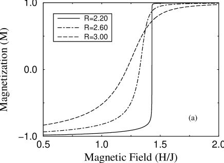
FIG. 1.: (a) Magnetization curves in $3$ dimensions for size $L=320$, and three values of disorder. The curves are averages of up to $48$ different random field configurations. Note the discontinuity in the magnetization for $R=2.20$. In finite size systems, the discontinuity in the magnetization curve occurs even for $R>R_{c}$ ($R_{c}=2.16$ in $3$ dimensions). (b) Scaling collapse (see text) of the magnetization curves in $3$ dimensions for size $L=320$. The disorders range from $R=2.35$ to $R=3.20$. The critical magnetization is chosen as $M_{c}=0.9$ from an analysis of the magnetization curves and is kept fixed during the collapse. The universal exponents are $\beta=0.036$, $\beta\delta=1.81$. The non–universal critical field $H_{c}=1.435$, critical disorder $R_{c}=2.16$, and rotation parameter $B=0.39$.

Figure 1a shows the magnetization curves obtained from our simulation in $3$ dimensions for several values of the disorder $R$. As the disorder $R$ is decreased, a discontinuity or jump in the magnetization curve appears where a single avalanche occupies a large fraction of the total system. In the thermodynamic limit this would be the infinite avalanche: the largest disorder at which it occurs is the critical disorder $R_{c}$. For finite size systems, like the ones we use in our simulation, we observe an avalanche which spans the system at a higher disorder, which gradually approaches $R_{c}$ as the system size grows.

FIG. 2.: $dM/dH$ curves in $3$ dimensions (a) Derivative of the magnetization $M$ with respect to the field $H$ for disorders $R=$ $2.35$, $2.4$, $2.45$, $2.5$, $2.6$, $2.7$, $2.85$, $3.0$, and $3.2$ (highest to lowest peak), (b) Scaling collapse of the data in (a) with $\beta=0.036$, $\beta\delta=1.81$, $B=0.39$, $H_{c}=1.435$, and $R_{c}=2.16$. While the curves are not collapsing onto a single curve, the quality of the collapse is quite similar to that found at similar distances from $R_{c}$ in mean field theory [19], for which we know analytically that scaling works as $R\to R_{c}$.

Figure 2 shows the slope $dM/dH$ and its scaling collapse. By using this derivative, the critical region is emphasized as the peak in the curve, and the dependence on the parameter $M_{c}$ drops out. The lower graphs in figures 1b and 2b show the scaling collapses of the magnetization and its slope. Clearly in neither case is all the data collapsing onto a single curve. This would be distressing, were it not for the fact that this also occurs in mean field theory [19] at a similar distance to the critical point.

Because the scaling of the magnetization is so bad, we use other quantities to estimate the critical exponents and the location of the critical point (tables I and III). Fixing these quantities, we use the collapse of the $dM/dH$ curves to extract the rotation $B$ mixing the experimental variables $r$ and $h$ into the scaling variable $h^{\prime}=h+Br$ (equation 5).

B Avalanche Size Distribution

1 Integrated Avalanche Size Distribution

FIG. 3.: Integrated avalanche size distribution curves in $3$ dimensions for $320^{3}$ spins and disorders $R=4.0,3.2$, and $2.6$. The last curve is at $R=2.25$, for a $1000^{3}$ spin system. The $320^{3}$ curves are averages over up to $16$ initial random field configurations. The inset shows the scaling collapse of the integrated avalanche size distribution curves in $3$ dimensions, using $r=(R-R_{c})/R$, $\tau+\sigma\beta\delta=2.03$, and $\sigma=0.24$, for sizes $160^{3}$, $320^{3}$, $800^{3}$, and $1000^{3}$, and disorders ranging from $R=2.25$ to $R=3.2$ ($R_{c}=2.16$). The two top curves in the collapse, at $R=3.2$, show noticeable corrections to scaling. The thick dark curve through the collapse is the fit to the data (see text). In the main figure, the distribution curves obtained from the fit to the collapsed data are plotted (thin lines) alongside the raw data (thick lines). The straight dashed line is the expected asymptotic power law behavior: $S^{-2.03}$, which does not agree with the measured slope of the raw data due to the shape of the scaling function (see text).

In our model the spins flip in avalanches: each spin can kick over one or more neighbors in a cascade. These avalanches come in different sizes. The integrated avalanche size distribution is the size distribution of all the avalanches that occur in one branch of the hysteresis loop (for $H$ from $-\infty$ to $\infty$). Figure 3[25] shows some of the raw data (thick lines) in $3$ dimensions. Note that the curves follow an approximate power law behavior over several decades. Even $50\%$ away from criticality (at $R=3.2$), there are still two decades of scaling, which implies that the critical region is large. In experiments, a few decades of scaling could be interpreted in terms of self-organized criticality (SOC). However, our model and simulation suggest that several decades of power law scaling can still be present rather ${\it far}$ from the critical point (note that the size of the critical region is non–universal). The slope of the log-log avalanche size distribution at $R_{c}$ gives the critical exponent $\tau+\sigma\beta\delta$. Notice, however, that the apparent slopes in figure 3 continue to change even after several decades of apparent scaling is obtained. The cutoff in the power law diverges as the critical disorder $R_{c}$ is approached. This cutoff size scales as $S\sim|r|^{-1/\sigma}$.

These critical exponents can be obtained by using a scaling collapse for the curves of figure 3, shown in the inset. The scaling form is

$$D_{int}(S,R)\sim S^{-(\tau+\sigma\beta\delta)}\ \bar{{\cal D}}^{(int)}_{+}(S^{\sigma}|r|)$$ (6)

where $\bar{{\cal D}}_{+}^{(int)}$ is the scaling function (the $+$ sign indicates that the collapsed curves are for $R>R_{c}$). We are sufficiently far from the critical point that corrections to scaling are important: as described in reference [19], we do collapses for small ranges of $R$ and then linearly extrapolate the best–fit critical exponents to $R_{c}$. We estimate from this curve that the critical exponents $\tau+\sigma\beta\delta=2.03$ and $\sigma=0.24$

The scaling function ${\cal D}_{+}^{(int)}(X)$ with $X=S^{\sigma}|r|$ is a universal prediction of our model. To facilitate comparisons with experiments, we fit a curve to the data collapse in the inset of figure 3. We have fit the scaling collapses in dimensions $3$, $4$, and $5$ to a phenomenological form of an exponential times a polynomial. In three dimensions, our fit is

$$\bar{{\cal D}}_{+}^{\it(int)}(X)\ =\ e^{-0.789X^{1/\sigma}}\ \times$$ (7)

$$(0.021+0.002X+0.531X^{2}-0.266X^{3}+0.261X^{4})$$ (8)

where $1/\sigma=4.20$. The distribution curves obtained using the above fit are plotted (thin lines in figure 3) alongside the raw data (thick lines). They agree remarkably well even far above $R_{c}$. We should recall though, that the fitted curve to the collapsed data can differ from the “real” scaling function even for large sizes and close to the critical disorder (in mean field [19] the error in the corresponding curve was about $10\%$).

The scaling function in the inset of figure 3 has a peculiar shape: it grows by a factor of ten before cutting off. The consequence of this bump in the shape is that in the simulations it takes many decades in the size distribution for the slope to converge to the asymptotic power law. This can be seen from the comparison between a straight line fit through the $R=2.25$ (billion spin) simulation in figure 3 and the asymptotic power law $S^{-2.03}$ obtained from extrapolating the scaling collapses (thick dashed straight line in the same figure). A similar bump exists in other dimensions and mean field as well. Figure 4 shows the scaling functions in different dimensions and in mean field. In this graph, the scaling functions are normalized to one and the peaks are aligned (the scaling forms allow this). The curves plotted in figure 4 are not raw data but fits to the scaling collapse in each dimensions, as was done in the inset of figure 3. For $5$, $4$, and $2$ dimensions, we have respectively:

$$\bar{{\cal D}}_{5}^{\it(int)}(X)\ =\ e^{-0.518X^{1/\sigma}}\ \times$$ (9)

$$(0.112+0.459X-0.260X^{2}+0.201X^{3}-0.050X^{4})$$ (10)

$$\bar{{\cal D}}_{4}^{\it(int)}(X)\ =\ e^{-0.954X^{1/\sigma}}\ \times$$ (11)

$$(0.058+0.396X+0.248X^{2}-0.140X^{3}+0.026X^{4})$$ (12)

$$\bar{{\cal D}}_{2}^{\it(int)}(X)\ =\ e^{-1.076X^{1/\sigma}}\ \times$$ (13)

$$(0.492-4.472X+14.702X^{2}-$$ (14)

$$20.936X^{3}+11.303X^{4})$$ (15)

with $1/\sigma=2.35,3.20$, and $10.0$. The errors in the fits are again in the 10% range, judging from mean–field theory [19].

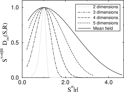
FIG. 4.: Integrated avalanche size distribution scaling functions in $2$, $3$, $4$, and $5$ dimensions, and mean field. The curves are fits (see text) to the scaling collapses done with exponents from Table I and corresponding calculations in two dimensions [20]. The peaks are aligned to fall on (1,1). Due to the “bump” in the scaling function the power law exponent can not be extracted from a linear fit to the raw data for reasonable simulation sizes [25].

In mean field theory (dimensions six and greater) a similar fit [19] to the analytical form of the scaling function above $R_{c}$ gives

$$\bar{{\cal D}}_{\rm MF}^{\it(int)}(X)\ =\ e^{-{X^{2}\over 2}}\ (0.204+0.482X-0.391X^{2}+$$ (16)

$$0.204X^{3}-0.048X^{4})$$ (17)

It is clear from the figure that the growing bump in the scaling curves as the dimension decreases is a foreshadowing of a zero in the scaling curve in two dimensions: this will be discussed further in reference [20].

2 Binned in $H$ Avalanche Size Distribution

The avalanche size distribution can also be measured at a field $H$ or in a small range of fields centered around $H$. We have measured this ${\it binned}$ in $H$ avalanche size distribution for systems at the critical disorder $R_{c}$ ($r=0$). To obtain the scaling form, we start from the distribution of avalanches at field $H$ and disorder $R$

$$D(S,R,H)\sim S^{-\tau}\ {\cal D}_{\pm}(S^{\sigma}|r^{\prime}|,|h|/|r^{\prime}|^{\beta\delta})$$ (18)

where as before ${\cal D}_{\pm}$ is the scaling function and $\pm$ indicates the sign of $r$.

The parameter $B$ of equation 5, which rotates the measured axes $(r,h)$ into the scaling axes $(r,h^{\prime}=h+Br)$, will be important [19] only for large avalanches of size $S>h^{-1/\sigma}$ near the critical point. In three and four dimensions, this does not affect our scaling collapses; in five dimensions we account for it [19].

The scaling function can be rewritten as ${\hat{\cal D}}_{\pm}\Bigl{(}S^{\sigma}|r|,(S^{\sigma}|r|)^{\beta\delta}|h|/|r|^{\beta\delta}\Bigr{)}$, where ${\hat{D}}_{\pm}$ is a new scaling function and $\pm$ represents whether $H$ is greater than or less than $H_{c}$ (i.e., $H$ rather than $R$). Letting $R\rightarrow R_{c}$, the scaling for the avalanche size distribution at the field $H$, measured at the critical disorder $R_{c}$ is:

$$D(S,H)\sim S^{-\tau}\ {\hat{\cal D}}_{\pm}(|h|S^{\sigma\beta\delta})$$ (19)

Figure 5a shows the binned in $H$ avalanche size distribution curves in $4$ dimensions, for values of $H$ below the critical field $H_{c}$. (The curves and analysis are similar in $3$ and $5$ dimensions; results in $4$ dimensions are used here for variety.) The simulation was done at the best estimate of the critical disorder $R_{c}$ ($4.1$ in $4$ dimensions). The binning in $H$ is logarithmic and started from an approximate critical field $H_{c}$ obtained from the magnetization curves; better estimates of $H_{c}$ are then obtained from the binned distribution data curves and their collapses. Our best estimate for the critical field $H_{c}$ in $4$ dimensions is $1.265\pm 0.007$. The scaling form for the logarithmically binned data is the same as in equation (19), if the log-binned data is normalized by the size of the bin. Figure 5b shows the scaling collapse for our data, both below and above the critical field $H_{c}$. The “top” collapse gives the shape of the ${\hat{\cal D}_{-}}$ ($H<H_{c}$) function, while the “bottom” collapse gives the ${\hat{\cal D}_{+}}$ ($H>H_{c}$) function. Above the critical field $H_{c}$, there are spanning avalanches in the system [28]. These are not included in the binned avalanche size distribution collapse shown in figure 5b.

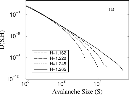
FIG. 5.: (a) Binned in $H$ avalanche size distribution in $4$ dimensions for a system of $80^{4}$ spins at $R=4.09$ ($R_{c}=4.10$). The critical field is $H_{c}=1.265$. The curves are averages over close to $60$ random field configuration. Only a few curves are shown. (b) Scaling collapse of the binned avalanche size distribution for $H<H_{c}$ (upper collapse) and $H>H_{c}$ (lower collapse). The critical exponents are $\tau=1.53$ and $\sigma\beta\delta=0.54$, and the critical field is $H_{c}=1.265$. The bins are at fields $1.162$, $1.185$, $1.204$, $1.220$, $1.234$, $1.245$, $1.254$, $1.276$, $1.285$, $1.296$, $1.310$, $1.326$, $1.345$, and $1.368$.

The exponent $\tau$ which gives the power law behavior of the binned avalanche size distribution is obtained from collapses of neighboring curves as described above [19], extrapolating to $H=H_{c}$. The exponent $\sigma\beta\delta$ is found to be very sensitive to $H_{c}$, while $\tau$ is not. We have therefore used the values of $\tau+\sigma\beta\delta$ and $\sigma$ from the integrated avalanche size distribution collapses, and $\tau$ from the binned avalanche size distribution collapses to further constrain $H_{c}$ (by constraining $\sigma\beta\delta$), and to calculate $\beta\delta$. The latter is then used to obtain collapses of the magnetization curves. We should mention here that $H_{c}$ in all the dimensions is difficult to find and that it is influenced by finite sizes. The values listed in Table III are the best estimates obtained from the largest system sizes we have. Nevertheless, systematic errors for $H_{c}$ could be larger than the errors given in Table III. These errors could produce systematic errors for $\sigma\beta\delta$ which depends on $H_{c}$, and for $\beta\delta$ which is calculated from $\sigma\beta\delta$: hence errors in these exponents could also be larger than the errors listed in Table II.

FIG. 6.: Linear fit to binned avalanche size distribution curve in $4$ dimensions, for a system of $80^{4}$ spins at $R_{c}=4.09$. The magnetic field is $H=1.265$. The straight solid line is a linear fit to the data for $S<13,000$ spins. The slope from the fit is $1.55$ (this varies by not more than $3\%$ as the range over which the fit is done is changed), while the exponent $\tau$ obtained from the collapses and the extrapolation in figure 5 is $1.53\pm 0.08$.

From figure 5b, we see that the two binned avalanche size distribution scaling function do not have a “bump” as does the scaling function for the integrated avalanche size distribution (inset in figure 3). Therefore, we expect that the exponent $\tau$ which gives the slope of the distribution in figure 5a can also be obtained by a linear fit through the data curve closest to the critical field. Figure 6 shows the curve for the $H=1.265$ bin (dashed curve) as well as the linear fit. The slope from the linear fit is $1.55$ while the value of $\tau$ obtained from the collapses and the extrapolation in figure 5 is $1.53\pm 0.08$.

C Avalanche Correlations

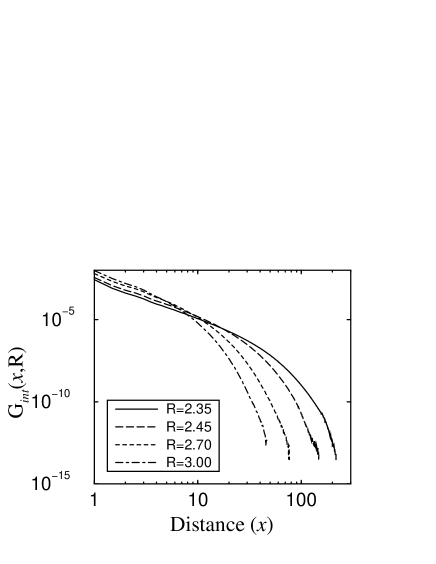
FIG. 7.: Avalanche correlation function integrated over the field $H$ in $3$ dimensions, for $L=320$. The curves are averages of up to $19$ random field configurations. The critical disorder $R_{c}$ is $2.16$.

The avalanche correlation function $G(x,R,H)$ measures the probability that the initial spin of an avalanche will trigger, in that avalanche, another spin a distance $x$ away. From the renormalization group description[13, 14], close to the critical point and for large distances $x$, the correlation function is given by:

$$G(x,R,H)\sim{1\over{x^{d-2+\eta}}}\ {\cal G}_{\pm}(x/{\xi(r,h)})$$ (20)

where $r$ and $h$ are respectively the reduced disorder and field, ${\cal G_{\pm}}$ ($\pm$ indicates the sign of $r$) is the scaling function, $d$ is the dimension, $\xi$ is the correlation length, and $\eta$ is called the “anomalous dimension”. Corrections can be shown to be subdominant [19]. The correlation length $\xi(r,h)$ is a macroscopic length scale in the system which is on the order of the mean linear extent of the largest avalanches. At the critical field $H_{c}$ (h=0) and near $R_{c}$, the correlation length scales like $\xi\sim|r|^{-\nu}$, while for small field $h$ it is given by

$$\xi\sim|r|^{-\nu}\ {\cal Y}_{\pm}(h/|r|^{\beta\delta})$$ (21)

where ${\cal Y}_{\pm}$ is a universal scaling function. The avalanche correlation function should not be confused with the cluster or “spin-spin” correlation which measures the probability that two spins a distance $x$ away have the same value. (The algebraic decay for this other, spin-spin correlation function at the critical point ($r=0$ and $h=0$), is $1/{x^{d-4+{\tilde{\eta}}}}$[13].)

We’ve mostly used, for historical reasons, a slightly different avalanche correlation function, which scales the same way as the “triggered” correlation function $G$ described above. Our function basically ignores the difference between the triggering spin and the other spins in the avalanche: alternatively, it calculates for avalanches of size $S$ the correlation function for pairs of spins, and then averages over all avalanches (weighting each avalanche equally). We’ve checked that our correlation function agrees to within 3% with the “triggered” correlation function described above, for $R>R_{c}$ in three dimensions and above. (In two dimensions, the two definitions differ more substantially, but appear to scale in the same way [20].)

We have measured the avalanche correlation function integrated over the field $H$, for $R>R_{c}$. For every avalanche that occurs between $H=-\infty$ and $H=+\infty$, we keep a count on the number of times a distance $x$ occurs in the avalanche. To decrease the computational time not every pair of spins is selected; instead we do a statistical sampling [21]. The spanning avalanches are not included in our correlation measurement. Figure 7 shows several avalanche correlation curves in $3$ dimensions for $L=320$. The scaling form for the avalanche correlation function integrated over the field $H$, close to the critical point and for large distances $x$, is obtained by integrating equation (20):

$$G_{\it int}(x,R)\sim\int{1\over{x^{d-2+\eta}}}\ {\cal G}_{\pm}\Bigl{(}x/{\xi(r,h)}\Bigr{)}\ dh$$ (22)

Using equation (21) and defining $u=h/|r|^{\beta\delta}$, equation (22) becomes:

$$G_{\it int}(x,R)\sim|r|^{\beta\delta}{x^{-(d-2+\eta)}}\int{\cal G}_{\pm}\Bigl{(}x/|r|^{-\nu}{\cal Y}_{\pm}(u)\Bigr{)}\ du$$ (23)

The integral ($\cal I$) in equation (23) is a function of $x|r|^{\nu}$ and can be written as:

$${\cal I}=(x|r|^{\nu})^{-\beta\delta/\nu}\ {\widetilde{\cal G}}_{\pm}(x|r|^{\nu})$$ (24)

to obtain the scaling form:

$$G_{\it int}(x,R)\sim{1\over x^{d+\beta/\nu}}\ {\widetilde{\cal G}}_{\pm}(x|r|^{\nu})$$ (25)

where we have used the scaling relation $(2-\eta)\nu=\beta\delta-\beta$ (see [13] for the derivation).

FIG. 8.: Scaling collapse of the avalanche correlation function integrated over the field $H$, in $3$ dimensions for $L=320$. The values of the disorders range from $R=2.35$ to $R=3.0$, with $R_{c}=2.16$. The exponents used in the collapse are $\nu=1.39\pm 0.20$ and $d+\beta/\nu=3.07\pm 0.30$. When collapses of neighboring curves are extrapolated to $R_{c}$, we get a slightly smaller value of $\nu=1.37\pm 0.18$.

FIG. 9.: Anisotropies in the avalanche correlation function. The curves are for a system of $320^{3}$ spins at $R=2.35$. Four curves are shown on the graph: one is the avalanche correlation function integrated over the field $H$ (as in figure 7), while the other three are measurements of the correlation along the three axis, the six face diagonals, and the four body diagonals. Avalanches involving more than four spins show no noticeable anisotropy: the critical point appears to have spherical symmetry. The same result is found in $2$ dimensions.

Figure 8 shows the integrated avalanche correlation curves collapse in $3$ dimensions for $L=320$ and $R>R_{c}$. The exponent $\nu$ is obtained from such collapses by extrapolating to $R=R_{c}$ as was done for other collapses [19]. The exponent $\beta/\nu$ can be obtained from these collapses too, but it is much better estimated from the magnetization discontinuity covered below. The value of $\beta/\nu$ listed in Table I is derived exclusively from the magnetization discontinuity collapses.

We have also looked for possible anisotropies in the integrated avalanche correlation function in $2$ and $3$ dimensions. The anisotropic integrated avalanche correlation functions are measured along “generalized diagonals”: one along the three axis, the second along the six face diagonals, and the third along the four body diagonals. We compare the integrated avalanche correlation function and the anisotropic integrated avalanche correlation functions to each other, and find no anisotropies in the correlation, as can be seen from figure 9.

D Spanning Avalanches

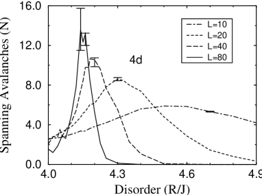
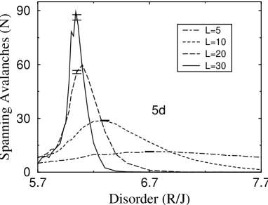
FIG. 10.: Spanning avalanches in $3$, $4$, and $5$ dimensions. (a) Number of spanning avalanches $N$ in $3$ dimensions, occurring in the system between $H=-\infty$ to $H=\infty$, as a function of the disorder $R$, for linear sizes $L$: $20$ (dot-dashed), $40$ (long dashed), $80$ (dashed), $160$ (dotted), and $320$ (solid). The critical disorder $R_{c}$ is at $2.16$. The error bars for each curve tend to be smaller than the error bar shown at the peak for disorders above the peak and larger for disorders below the peak. They are not given here for clarity. Note that the number of avalanches increases only slightly as the size is increased. (b) Number of spanning avalanches in $4$ dimensions. The critical disorder is $4.1$. (c) Number of spanning avalanches in $5$ dimensions. The critical disorder is $5.96$. Both in $4$ and $5$ dimensions, the peaks grow and shift towards $R_{c}$ as the size of the system is increased. (d) Collapse of the spanning avalanche curves in $4$ dimensions for linear sizes $L=20,40$, and $80$. The exponents are $\theta=0.32$ and $\nu=0.89$, and the critical disorder is $R_{c}=4.10$. The collapse is done using $r=(R_{c}-R)/R$.

The critical disorder $R_{c}$ was defined earlier as the disorder $R$ at which an ${\it infinite}$ avalanche first appears in the system, in the thermodynamic limit, as the disorder is lowered. At that point, the magnetization curve will show a discontinuity at the magnetization $M_{c}(R_{c})$ and field $H_{c}(R_{c})$. For each disorder $R$ below the critical disorder, there is ${\it one}$ infinite avalanche that occurs at a critical field $H_{c}(R)>H_{c}(R_{c})$ [13, 14], while above $R_{c}$ there are only finite avalanches. This is the behavior for an infinite size system. In a finite size system far below and above $R_{c}$ the above picture is still true, but close to the critical disorder, as we approach the transition, the avalanches get larger and larger, and there will be a first point where one of them will span the system from one side to another in at least one direction. This avalanche is not the infinite avalanche; if the system was larger, this avalanche would typically be non–system spanning. Such an avalanche (which spans the system) we call a spanning avalanche.

In our numerical simulation, we find that for finite sizes $L$, there are not one but ${\it many}$ such avalanches in $4$ and $5$ dimensions (and maybe $3$), and that their number increases as the system size increases [29]. Figures 10(a-c) show the number of spanning avalanches as a function of disorder $R$, for different sizes and dimensions. In $4$ and $5$ dimensions, the spanning avalanche curves become more narrow as the system size is increased. Also, the peaks shift toward the critical value of the disorder ($4.1$ and $5.96$ respectively), and the number of spanning avalanches at $R_{c}$ increases. This suggests that in $4$ and $5$ dimensions, for $L\rightarrow\infty$, there will be one infinite avalanche below $R_{c}$, none above, and an infinite number of infinite, spanning avalanches at the critical disorder $R_{c}$. In $3$ dimensions, the results are not conclusive, as noted both from figure 10a and from the value of the spanning avalanche exponent $\theta=0.15\pm 0.15$ defined below: a value of $\theta=0$ is consistent with one infinite or spanning avalanche at $R_{c}$ as $L\rightarrow\infty$. It is clear that $\theta=0$ in two dimensions, since spanning avalanches can’t interpenetrate: it’s thus plausible that $\theta$ is near zero in three dimensions because it must vanish one dimension lower.

In percolation, a similar multiplicity of infinite clusters [30, 31] as the system size is increased is found for dimensions above six which is the upper critical dimension (UCD). The UCD is the dimension at and above which the mean field exponents are valid. Below six dimensions, there is only one such infinite cluster in percolation. The existence of a diverging number of infinite clusters in percolation is associated with the breakdown of the hyperscaling relation above six dimensions. Since a hyperscaling relation is a relation between critical exponents that includes the dimension $d$ of the system, it is always only satisfied up to and including the upper critical dimension. In our system, the upper critical dimension is also six, but we find spanning avalanches in dimensions even below that. In a comment by Maritan et al.[29], it was suggested that our system should satisfy the hyperscaling relation $d\nu-\beta=1/\sigma$ found in percolation [31]. But since our system has spanning avalanches below the upper critical dimension, this hyperscaling relation breaks down below six dimensions. Due to the existence of many spanning avalanches near $R_{c}$, the new “violation of hyperscaling” relation for dimensions three and above becomes [13]:

$$(d-\theta)\nu-\beta=1/\sigma$$ (26)

where $\theta$ is the “breakdown of hyperscaling” or spanning avalanches exponent defined below. One can check that our exponents in $3$, $4$, and $5$ dimensions and mean field satisfy this equation (see Tables I and II).

For the simulation, we define a spanning avalanche to be an avalanche that spans the system in a particular direction. We average over all the directions to obtain better statistics. Depending on the size and dimension of the system and the distance from the critical disorder, the number of spanning avalanches for a particular value of disorder $R$ is obtained by averaging over as few as $5$ to as many as $2000$ different random field configurations. We define the exponent $\theta$ such that the number $N$ of spanning avalanches, at the critical disorder $R_{c}$, increases with the linear system size as: $N\sim L^{\theta}$ ($\theta>0$). The finite size scaling form[27] for the number of spanning avalanches close to the critical disorder is:

$$N(L,R)\sim L^{\theta}\ {\cal N}_{\pm}(L^{1/\nu}|r|)$$ (27)

where $\nu$ is the correlation length exponent and ${\cal N}_{\pm}$ is the corresponding scaling function ($\pm$ indicates the sign of $r$). The collapse is shown in figure 10d. (We show the collapses in $4$ dimensions here since the existence of spanning avalanches in $3$ dimensions is not conclusive.) These values are used along with the results from other collapses to obtain Table I. In the analysis of the avalanche size distribution, magnetization, and correlation functions for $R>R_{c}$, how close we chose to come to the critical disorder $R_{c}$ was determined by the spanning avalanches: we include no values $R$ below the first value which exhibited a spanning avalanche.

E Magnetization Discontinuity

We have mentioned earlier that in the thermodynamic limit, at and below the critical disorder $R_{c}$, there is a critical field $H_{c}(R)>H_{c}(R_{c})$ at which the infinite avalanche occurs. Close to the critical transition, for small $r<0$, the change in the magnetization due to the infinite avalanche scales as (equation (4)):

$$\Delta M(R)\sim\ r^{\beta}$$ (28)

where $r=(R_{c}-R)/R$, while above the transition, there is no infinite avalanche.

In finite size systems, the transition is not as sharp: we have spanning avalanches above the critical disorder. If we measure the change in the magnetization due to all the spanning avalanches as a function of disorder $R$ at various system sizes $L$, we expect it will obey finite–size scaling (as did the number of spanning avalanches):

$$\Delta M(L,R)\sim\ |r|^{\beta}\ \Delta{\cal M}_{\pm}(L^{1/\nu}|r|)$$ (29)

where $\Delta{\cal M}_{\pm}$ is a universal scaling function. (The parameter $B$ here (equation 5) is unimportant [19] because we $\Delta M$ is measured at $h^{\prime}=0$.) Defining a new universal scaling function $\Delta\widetilde{\cal M}_{\pm}$:

$$\Delta{\cal M}_{\pm}(L^{1/\nu}|r|)\equiv\ (L^{1/\nu}|r|)^{-\beta}\ \Delta\widetilde{\cal M}_{\pm}(L^{1/\nu}|r|)$$ (30)

we obtain the scaling form:

$$\Delta M(L,R)\sim\ L^{-\beta/\nu}\ \Delta{\widetilde{\cal M}_{\pm}}(L^{1/\nu}|r|)$$ (31)

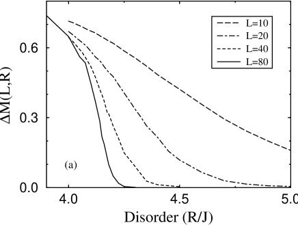
FIG. 11.: Jump in the magnetization, in $4$ dimensions (a) Change in the magnetization due to the spanning avalanches in $4$ dimensions, for several linear sizes $L$, as a function of the disorder $R$. (b) Scaling collapse of the curves in (a) using $r=(R_{c}-R)/R$. The exponents are $1/\nu=1.12$ and $\beta/\nu=0.19$, and the critical disorder is $R_{c}=4.1$.

Figures 11a and 11b show the change in the magnetization due to the spanning avalanches in $4$ dimensions, and a scaling collapse of that data (similar results exist in $3$ and $5$ dimensions). Notice that as the system size increases, the curves approach the $|r|^{\beta}$ behavior. The exponents $1/\nu$ and $\beta/\nu$ are extracted from scaling collapses (figure 11b) and extrapolated to $R_{c}$ [19]. The value of $\beta$ is calculated from $\beta/\nu$ and the knowledge of $\nu$, and is the value used for collapses of the magnetization curves (discussed earlier).

F Moments of the Avalanche Size Distribution

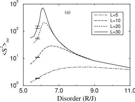
FIG. 12.: Second moments. (a) Second moments of the avalanche size distribution integrated over the field $H$, in $5$ dimensions. Error bars are largest for smaller disorders (shown on the curves). The curves have between $24$ and $50$ points, and the value of the second moment for each disorder is averaged over $3$ to $100$ different random field configurations. (b) Scaling collapse of the $L=10,20$, and $30$ curves from (a) using $r=(R_{c}-R)/R$. The exponents are $1/\nu=1.47$ and $\rho=-(\tau+\sigma\beta\delta-3)/\sigma\nu=2.95$, and the critical disorder is $R_{c}=5.96$.

The second moment of the integrated avalanche size distribution has a finite–size scaling form

$$\langle S^{2}{\rangle}_{\it int}\sim L^{-(\tau+\sigma\beta\delta-3)/\sigma\nu}\ {\widetilde{\cal S}}_{\pm}^{(2)}(L^{1/\nu}|r|)$$ (32)

where $L$ is the linear size of the system, $r$ is the reduced disorder, $\widetilde{\cal S}_{\pm}^{(2)}$ is the scaling function, and $\nu$ is the correlation length exponent. We can similarly define the third and fourth moment, with the exponent $-(\tau+\sigma\beta\delta-3)/\sigma\nu$ replaced by $-(\tau+\sigma\beta\delta-4)/\sigma\nu$ and $-(\tau+\sigma\beta\delta-5)/\sigma\nu$ respectively. Figures 12a and 12b show the second moments data in $5$ dimensions for sizes $L=5,10,20,$ and $30$, and a collapse (again, results in $3$ and $4$ dimensions are similar and we have chosen to show the curves in $5$ dimensions for variety). The curves are normalized by the average avalanche size integrated over all fields $H$: $\int_{-\infty}^{+\infty}\int_{1}^{\infty}S\ D(S,R,H,L)\ dS\ dH$. The spanning avalanches are not included in the calculation of the moments. We omit the $L=5$ curve from the collapse; it doesn’t collapse with the others well, presumably because of subdominant finite size effects. The exponents for the third and fourth moment can be calculated from those of the second moment, and we find that they agree with the values obtained from their respective collapses.

G Avalanche Time Measurement

The exponents we have measured so far are static scaling exponents: they do not depend on the dynamics of the model. If we measure the time an avalanche takes to occur, we are making a dynamical measurement. The time measurement in the numerical simulation is done by increasing the time clock by one for each shell of spins in the avalanche. That is, we implement time as a synchronous dynamics, where in each time step all unstable spins from the previous step are flipped. The scaling relation between the time $t$ it takes an avalanche to occur and the linear size $\xi$ of the avalanche defines the critical exponent $z$ [32, 33]:

$$t\sim\xi^{z}$$ (33)

The exponent $z$ is known as the dynamical critical exponent. Equation (33) gives the scaling for the time it takes for a spin to “feel” the effect of another a distance $\xi$ away. Since the correlation length $\xi$ scales like $r^{-\nu}$ close to the critical disorder, and the characteristic size $S$ as $r^{-1/\sigma}$, the time $t$ then scales with avalanche size as:

$$t\sim S^{\sigma\nu z}$$ (34)

In our simulation, we measure the distribution of times for each avalanche size $S$. The distribution of times $D_{t}(S,R,H,t)$ for an avalanche of size $S$ close to the critical field $H_{c}$ and critical disorder $R_{c}$ is

$$D_{t}(S,R,H,t)\sim S^{-q}\ {\bar{\cal D}}_{\pm}^{(t)}(S^{\sigma}|r|,h/|r|^{\beta\delta},t/S^{\sigma\nu z})$$ (35)

where $q=\tau+\sigma\nu z$, and is defined such that

$$\int_{-\infty}^{+\infty}\!\!\int_{1}^{\infty}D_{t}(S,R,H,t)\ dH\ dt\ =\$$ (36)

$$S^{-(\tau+\sigma\beta\delta)}\ {\bar{\cal D}}_{\pm}^{(int)}(S^{\sigma}|r|)$$ (37)

where ${\bar{\cal D}}_{\pm}^{(int)}$ was defined in the integrated avalanche size distribution section. The avalanche time distribution integrated over the field $H$, at the critical disorder ($r=0$) is:

$$D_{t}^{(int)}(S,t)\ \sim\ t^{-{(\tau+\sigma\beta\delta+\sigma\nu z)/\sigma\nu z}}\ {\cal D}_{t}^{(int)}(t/S^{\sigma\nu z})$$ (38)

which obtained from equation (35) (reference [19]).

FIG. 13.: (a) Avalanche time distribution curves in $3$ dimensions, for avalanche size bins from about $2000$ to $40000$ spins (from upper left to lower right corner). The system size is $800^{3}$ at $R=2.26$. The curves are from only one random field configuration. (b) Scaling collapse of curves in (a). The values of the exponents are $\sigma\nu z=0.57$ and $(\tau+\sigma\beta\delta+\sigma\nu z)/\sigma\nu z=4.0$.

Figures 13a and 13b show the avalanche time distribution integrated over the field $H$ for different avalanche sizes, and a collapse of these curves using the above scaling form, for a $800^{3}$ system at $R=2.260$ (just above the range where spanning avalanches occur). The data is saved in logarithmic size bins, each about $1.2$ times larger than the previous one. The time is also measured logarithmically (next bin is $1.1$ times larger than the previous one). The extracted value for $z$ in $3$ dimensions is $1.68\pm 0.07$. The results for other dimensions are listed in Table I.

H Tables of Results

measured exponents	$3$d		$4$d		$5$d		mean field
$1/\nu$	0.71$\,\pm\,$	0.09	1.12$\,\pm\,$	0.11	1.47$\,\pm\,$	0.15	2
$\theta$	0.015$\,\pm\,$	0.015	0.32$\,\pm\,$	0.06	1.03$\,\pm\,$	0.10	1
$(\tau+\sigma\beta\delta-3)/\sigma\nu$	-2.90$\,\pm\,$	0.16	-3.20$\,\pm\,$	0.24	-2.95$\,\pm\,$	0.13	-3
$1/\sigma$	4.2$\,\pm\,$	0.3	3.20$\,\pm\,$	0.25	2.35$\,\pm\,$	0.25	2
$\tau+\sigma\beta\delta$	2.03$\,\pm\,$	0.03	2.07$\,\pm\,$	0.03	2.15$\,\pm\,$	0.04	9/4
$\tau$	1.60$\,\pm\,$	0.06	1.53$\,\pm\,$	0.08	1.48$\,\pm\,$	0.10	3/2
$d+\beta/\nu$	3.07$\,\pm\,$	0.30	4.15$\,\pm\,$	0.20	5.1$\,\pm\,$	0.4	7 (at $d_{c}=6$)
$\beta/\nu$	0.025$\,\pm\,$	0.020	0.19$\,\pm\,$	0.05	0.37$\,\pm\,$	0.08	1
$\sigma\nu z$	0.57$\,\pm\,$	0.03	0.56$\,\pm\,$	0.03	0.545$\,\pm\,$	0.025	1/2

TABLE I.: Universal critical exponents. Values for the exponents extracted from scaling collapses in $3$, $4$, and $5$ dimensions. The mean field values are calculated analytically[12, 13]. $\nu$ is the correlation length exponent and is found from collapses of avalanche correlations, number of spanning avalanches, and moments of the avalanche size distribution data. The exponent $\theta$ is a measure of the number of spanning avalanches and is obtained from collapses of that data. $(\tau+\sigma\beta\delta-3)/\sigma\nu$ is obtained from the second moments of the avalanche size distribution collapses. $1/\sigma$ is associated with the cutoff in the power law distribution of avalanche sizes integrated over the field $H$, while $\tau+\sigma\beta\delta$ gives the slope of that distribution. $\tau$ is obtained from the binned avalanche size distribution collapses. $d+\beta/\nu$ is obtained from avalanche correlation collapses and $\beta/\nu$ from magnetization discontinuity collapses. $\sigma\nu z$ is the exponent combination for the time distribution of avalanche sizes and is extracted from that data. Error bars are based on variations in the results based on different approaches to the analysis: statistical fluctuations are typically smaller.

calculated exponents	$3$d		$4$d		$5$d		mean field
$\sigma\beta\delta$	0.43$\,\pm\,$	0.07	0.54$\,\pm\,$	0.08	0.67$\,\pm\,$	0.11	3/4
$\beta\delta$	1.81$\,\pm\,$	0.32	1.73$\,\pm\,$	0.29	1.57$\,\pm\,$	0.31	3/2
$\beta$	0.035$\,\pm\,$	0.028	0.169$\,\pm\,$	0.048	0.252$\,\pm\,$	0.060	1/2
$\sigma\nu$	0.34$\,\pm\,$	0.05	0.28$\,\pm\,$	0.04	0.29$\,\pm\,$	0.04	1/4
$\eta=2+(\beta-\beta\delta)/\nu$	0.73$\,\pm\,$	0.28	0.25$\,\pm\,$	0.38	0.06$\,\pm\,$	0.51	0

TABLE II.: Values for exponents in $3$, $4$, and $5$ dimensions that are not extracted directly from scaling collapses, but instead are derived from Table I and the exponent relations (see [13]). The mean field values are obtained analytically [12, 13]. Both $\sigma\beta\delta$ and $\beta\delta$ could have larger systematic errors than the errors listed here. See the binned avalanche size distribution section for details.

	$3$d		$4$d		$5$d		mean field
$R_{c}$	2.16$\,\pm\,$	0.03	4.10$\,\pm\,$	0.02	5.96$\,\pm\,$	0.02	0.79788456
$H_{c}$	1.435$\,\pm\,$	0.004	1.265$\,\pm\,$	0.007	1.175$\,\pm\,$	0.004	0
$B$	0.39$\,\pm\,$	0.08	0.46$\,\pm\,$	0.05	0.23$\,\pm\,$	0.08	0

TABLE III.: Non-universal scaling variables. Numerical values for the critical disorders and fields, and the rotation parameter $B$ (equation 5), in $3$, $4$, and $5$ dimensions extracted from scaling collapses. The critical disorder is obtained from collapses of the spanning avalanches and the second moments of the avalanche size distribution. The critical field is obtained from the binned avalanche size distribution and the magnetization curves. $H_{c}$ is affected by finite sizes, and systematic errors could be larger than the ones listed here. The mean field values are calculated analytically[12, 13]. The rotation $B$ is obtained from the $dM/dH$ collapses.

V Comparison with the analytical results

Here we compare the simulation results with the renormalization group analysis of the same system [13, 14]. According to the renormalization group the upper critical dimension (UCD), at and above which the critical exponents are equal to the mean field values, is six. Close to the UCD, it is possible to do a $6-\epsilon$ expansion, and obtain estimates for the critical exponents and the magnetization scaling function, which can then be compared with our numerical results.

FIG. 14.: Comparison between the critical exponents from the simulation and the $\epsilon$ expansion Numerical values (filled symbols) of the exponents $\tau+\sigma\beta\delta$, $\tau$, $1/\nu$, $\sigma\nu z$, and $\sigma\nu$ (circles, diamond, triangles up, squares, and triangle left) in $2$, $3$, $4$, and $5$ dimensions. The empty symbols are values for these exponents in mean field (dimension 6). Exponents in two dimensions are discussed elsewhere [25, 19, 20]. Note that the value of $\tau$ in $2$d conjectured value [25]. We have simulated sizes up to $30000^{2}$, $1000^{3}$, $80^{4}$, and $50^{5}$, where for $320^{3}$ for example, more than $700$ different random field configurations were measured. The long-dashed lines are the $\epsilon$ expansions to first order for the exponents $\tau+\sigma\beta\delta$, $\tau$, $\sigma\nu z$, and $\sigma\nu$. The short-dashed lines are Borel sums[34] for $1/\nu$, as discussed in [25]. The lowest is the variable-pole Borel sum from LeGuillou et al.[34], the middle uses the method of Vladimirov et al. to fifth order, and the upper uses the method of LeGuillou et al., but without the pole and with the correct fifth order term. The error bars denote systematic errors in finding the exponents from extrapolation of the values obtained from collapses of curves at different disorders $R$. Statistical errors are smaller.

Figure 14 shows the numerical and analytical results for five of the critical exponents obtained in dimensions two to six (in six dimensions, the values are the mean field ones). The other exponents can be obtained from scaling relations[13]. The exponent values in figure 14 are obtained by extrapolating the results of scaling collapses to either $R\rightarrow R_{c}$ or $1/L\rightarrow 0$ (see [19]). The long-dashed lines are the $\epsilon$ expansions to first order for $\tau+\sigma\beta\delta$, $\tau$, $\sigma\nu z$, and $\sigma\nu$. The three short-dashed lines[13] are Borel sums[34] for $1/\nu$. Notice that the numerical values converge nicely to the mean field predictions, as the dimension approaches six, and that the agreement between the numerical values and the $\epsilon$ expansion is quite impressive.

FIG. 15.: Comparison between simulated $dM/dH$ curves in $5$ dimensions, and the $dM/dH$ curve obtained from the $\epsilon$ expansion. The thick dashed line shows the prediction of the $\epsilon$ expansion to third order in $\epsilon$ for the slope of the magnetization curve $dM/dH$ in five dimensions. The theoretical curve is a parametric form [35] taken from the analysis of the ordinary, pure, thermal Ising model in three dimensions [14]. The six simulation curves (thin lines) are for a system of $30^{5}$ spins at disorders $7.0,7.3,$ and $7.5$ ($R_{c}=5.96$ in $5$ dimensions), and for a system of $50^{5}$ spins at disorders $6.3,6.4$, and $6.5$. The latter curves are closer to the theoretical dashed line). All the curves have been stretched/shrunk in the horizontal and vertical direction and shifted horizontally to lie on each other.

The $\epsilon$ expansion can be an even more powerful tool if it can predict the scaling functions. This has been done for the magnetization scaling function of the pure Ising model in $4-\epsilon$ dimensions [36, 35]. Since the $\epsilon$ expansion for our model is the same as the one for the equilibrium RFIM [13], and the latter has been mapped to all orders in $\epsilon$ to the corresponding expansion of the regular Ising model in two lower dimensions [13, 37, 38], we can use the results obtained in [36, 35]. This is done in figure 15, which shows the comparison between the $dM/dH$ curves obtained in $5$ dimensions and the predicted scaling function for $dM/dH$, to third order in $\epsilon$, where $\epsilon=1$ in $5$ dimensions (see [35]). As we see, the agreement is very good in the scaling region (close to the peaks).

VI Summary

We have used the zero temperature random field Ising model, with a Gaussian distribution of random fields, to model a random system that exhibits hysteresis. We found that the model has a transition in the shape of the hysteresis loop, and that the transition is critical. The tunable parameters are the amount of disorder $R$ and the external magnetic field $H$. The transition is marked by the appearance of an infinite avalanche in the thermodynamic system. Near the critical point, ($R_{C}$, $H_{C}$), the scaling region is quite large: the system can exhibit power law behavior for several decades, and still not be near the critical transition. This is important to keep in mind whenever experimental data are analyzed: decades of scaling need not imply self–organized criticality.

We have extracted critical exponents for the magnetization, the avalanche size distribution (integrated over the field and binned in the field), the moments of the avalanche size distribution, the avalanche correlation, the number of spanning avalanches, and the distribution of times for different avalanche sizes. These values are listed in Table I, and were obtained as an average of the extrapolation results (to $R\rightarrow R_{c}$ or $L\rightarrow\infty$) from several measurements [19]. As shown earlier, the numerical results compare well with the $\epsilon$ expansion [13, 14]. Comparisons to experimental Barkhausen noise measurements [25] are very encouraging.

We acknowledge the support of DOE Grant #DE-FG02-88-ER45364 and NSF Grant #DMR-9805422. We thank Matt Kuntz for noticing and fixing the differences between our analytical and numerical avalanche correlation functions. We would like to thank Sivan Kartha, Bruce Roberts, M. E. J. Newman, J. A. Krumhansl, J. Souletie, and M. O. Robbins for helpful conversations. This work was conducted partly on the SP1 and SP2 at the Cornell Theory Center (funded in part by the National Science Foundation, by New York State, and by IBM), and partly on IBM 560 workstations and an IBM J30 SMP system (both donated by IBM). We would like to thank CNSF and IBM for their support. Further pedagogical information using Mosaic is available at http://www.lassp.cornell.edu/sethna/hysteresis/ and http://SimScience.org/crackling/.

REFERENCES

- [1] J. D. Shore, M. Holzer, and J. P. Sethna, Phys. Rev. B 46, 11376 (1992); J. D. Shore and J. P. Sethna, Phys. Rev. B 43, 3782 (1991); T. Riste and D. Sherrington, Phase Transitions and Relaxation in Systems with Competing Energy Scales (Proc. NATO Adv. Study Inst., Geilo, Norway, April 13-23, 1993), and references therein; M. Mézard, G. Parisi, M. A. Virasoro, Spin Glass Theory and Beyond (World Scientific, Singapore, 1987), and references therein; K. H. Fischer and J. A. Hertz, Spin Glasses (Cambridge University Press, Cambridge, 1993), and references therein; G. Grinstein and J. F. Fernandez, Phys. Rev. B 29, 6389 (1984); J. Villain, Phys. Rev. Lett. 52, 1543 (1984); D. S. Fisher, Phys. Rev. Lett. 56, 416 (1986).
- [2] D. Jiles, Introduction to Magnetism and Magnetic Materials (Chapman and Hall, New York, 1991).
- [3] J. C. McClure, Jr. and K. Schröder, CRC Crit. Rev. Solid State Sci. 6, 45 (1976);
- [4] K. P. O’Brien and M. B. Weissman, Phys. Rev. E 50, 3446 (1994), and references therein; K. P. O’Brien and M. B. Weissman, Phys. Rev. A 46, R4475 (1992); U. Lieneweg and W. Grosse-Nobis, Intern. J. Magnetism 3, 11 (1972); Djordje Spasojević, Srdjan Bukvić, Sava Milošević, and H. Eugene Stanley, preprint (1995).
- [5] J. S. Urbach, R. C. Madison, and J. T. Markert, Phys. Rev. Lett. 75, 276 (1995).
- [6] P. J. Cote and L. V. Meisel, Phys. Rev. Lett. 67, 1334 (1991); L. V. Meisel and P. J. Cote, Phys. Rev. B 46, 10822 (1992);
- [7] P. Bak, C. Tang, and K. Wiesenfeld, Phys. Rev. Lett. 59, 381 (1987); Phys. Rev. A 38, 364 (1988).
- [8] S. Field, J. Witt, and F. Nori, Phys. Rev. Lett. 74, 1206 (1995), (vortex lines).
- [9] W. Wu and P. W. Adams, Phys. Rev. Lett. 74, 610 (1995), (resistance measurement in a superconductor).
- [10] M. P. Lilly, P. T. Finley, and R. B. Hallock, Phys. Rev. Lett. 71, 4186 (1993), (helium in Nuclepore).
- [11] A. Berger, not published.
- [12] J. P. Sethna, K. A. Dahmen, S. Kartha, J. A. Krumhansl, B. W. Roberts, and J. D. Shore, Phys. Rev. Lett. 70, 3347 (1993).
- [13] K. A. Dahmen and J. P. Sethna, accepted for publication in PRB; K. A. Dahmen, Ph.D. Thesis, Cornell University (1995).
- [14] K. A. Dahmen and J. P. Sethna, Phys. Rev. Lett. 71, 3222 (1993).
- [15] O. Narayan and D. S. Fisher, Phys. Rev. Lett. 68, 3615 (1992) and Phys. Rev. B 46, 11520 (1992); D. Ertaş and M. Kardar, Phys. Rev. E 49, R2532 (1994); C. Myers and J.P. Sethna, Phys. Rev. B 47 11171 (1993) and Phys. Rev. B 47 11194 (1993).
- [16] T. Nattermann, S. Stepanow, L. H. Tang and H. Leschhorn, J. Phys. II France 2, 1483 (1992); O. Narayan and D. S. Fisher, Phys. Rev. B 48, 7030 (1993).
- [17] C. M. Coram, A. E. Jacobs, N. Heinig, and K. B. Winterbon, Phys. Rev. B 40, 6992 (1989).
- [18] E. Vives, J. Goicoechea, J. Ortín, and A. Planes, Phys. Rev. E 52, R5 (1995). E. Vives and A. Planes, Phys. Rev. B 50, 3839 (1994). A comparison between our simulation and their results show that the dimensional results agree quite nicely. However, in dimensions, there are large differences, which we believe occur because of the small system sizes used by the authors for their simulation (only up to , but the reported their results first). We have seen that our results are very size dependent. We would expect for a system of spins to find a critical disorder , as was found by these authors; however, we find after increasing the system size that the critical disorder is or lower [19, 20]. These authors also explore the zero temperature random bond Ising model, which they show also exhibits a critical transition in the shape of the hysteresis loop, where the mean bond strength is analogous to our disorder . They give numerical evidence that the random bond Ising model is in the same universality class as our random field model. We argue elsewhere on symmetry grounds that this is likely the case [14], and that the experimentally more relevant random–anisotropy model is also likely described by our critical point.
- [19] O. Perković, K. A. Dahmen, and J. P. Sethna, Condensed-Matter Archive preprint #9609072.
- [20] M. C. Kuntz, O. Perković, and J. P. Sethna, manuscript in preparation.
- [21] J. P. Sethna, O. Perković, M. C. Kuntz, K. A. Dahmen, and B. W. Roberts, “Hysteresis, Avalanches, and Noise: Numerical Methods”, manuscript in preparation.
- [22] D. Dhar, P. Shukla, and J. P. Sethna, J. Phys. A 30 5259 (1997).
- [23] J.–G. Zhu and H. Neal Bertram, J. Appl. Phys. 69, 4709 (1991) studied a hexagonal two-dimensional model with in-plane magnetization, ferromagnetic bonds with the four neighbors along the field direction and antiferromagnetic (or missing) bonds with the two neighbors perpendicular to the field.
- [24] Hong Ji and Mark O. Robbins, Phys. Rev. B 46, 14519 (1992), and references therein. Robbins and Ji initiated the study of this particular model, except that they use it to study the closely related interface depinning problem (which does not allow avalanches to start except next to existing flipped spins).
- [25] O. Perković, K. A. Dahmen, and J. P. Sethna, Phys. Rev. Lett. 75, 4528 (1995).
- [26] K. G. Wilson, Phys. Rev. B 4, 3174, 3184 (1971); K. G. Wilson and M. E. Fisher, Phys. Rev. Lett. 28, 240 (1972); K. G. Wilson and J. Kogut, Phys. Rep. C 12, 75 (1974); J.M. Yeomans, Statistical Mechanics of Phase Transitions (Clarendon Press, Oxford 1992); M. Plischke and B. Bergersen, Equilibrium Statistical Physics (Prentice Hall, NJ 1989); S. Ma, Modern Theory of Critical Phenomena (Benjamin, Massachusetts, 1976); M. E. Fisher in Critical Phenomena, Lecture Notes in Physics, Vol. 186, Ed. F. J. W. Hahne (Springer–Verlag, Berlin 1983).
- [27] For a good introduction on static scaling and finite size scaling, see: N. Goldenfeld, Lectures on Phase Transition and the Renormalization Group (Addison Wesley, 1992). M. N. Barber in Phase Transitions and Critical Phenomena, Vol. 8, eds. C. Domb and J. L. Lebowitz (Academic Press, NY, 1983).
- [28] In and dimensions, below the critical field , we have not found any spanning avalanches. In dimensions, spanning avalanches appeared below the critical field . We believe this is due to the small system size () used for the dimensional simulation. We however, do not expect substantial corrections to the exponents derived from that data.
- [29] The divergence in the number of spanning avalanches near and the association with hyperscaling was originally discussed in our response to a comment by A. Maritan, M. Cieplak, M. R. Swift and J. Banavar, Phys. Rev. Lett. 72, 946 (1994); J. P. Sethna, K. A. Dahmen, S. Kartha, J. A. Krumhansl, O. Perković, B. W. Roberts, and J. D. Shore, Phys. Rev. Lett. 72, 947 (1994).
- [30] L. de Arcangelis, J. Phys. A 20, 3057 (1987); A. Coniglio, Springer Proc. Phys., 5, 84 (1985).
- [31] D. Stauffer and A. Aharony, Introduction to Percolation Theory, revised second edition (Taylor & Francis, London, Bristol, PA 1994).
- [32] P. C. Hohenberg and B. I. Halperin, Rev. Mod. Phys. 49,(1977).
- [33] J. J. Binney, N. J. Dowrick, A. J. Fisher, and M. E. J. Newman, The Theory of Critical Phenomena (Clarendon Press, Oxford, 1992). S. Ma, Modern Theory of Critical Phenomena (Benjamin, Massachusetts, 1976).
- [34] H. Kleinert, J. Neu, V. Schulte-Frohlinde, K.G. Chetyrkin, and S. A. Larin (Phys. Lett. B 272, 39 (1991) and erratum in Phys. Lett. B 319, 545 (1993)) provide the expansion for the pure, equilibrium Ising exponents to fifth order in . A. A. Vladimirov, D. I. Kazakov, and O. V. Tarasov, (Sov. Phys. JETP 50 (3), 521 (1979) and references therein) introduce a Borel resummation method with one parameter, which is varied to accelerate convergence. J.C. LeGuillou and J. Zinn-Justin (Phys. Rev. B 21, 3976 (1980)) do a coordinate transformation with a pole at , and later (J. Physique Lett. 46, L137 (1985) and J. Physique 48, 19 (1987)) make the placement of the pole a variable parameter (leading to a total of four real acceleration parameters for a fifth order expansion!). Unfortunately, LeGuillou et al. used a form for the fifth order term which turned out to be incorrect (Kleinert, above). The expansion is an asymptotic series, which need not determine a unique underlying function (J. Zinn-Justin “Quantum Field Theory and Critical Phenomena”, 2nd edition, Clarendon Press, Oxford (1993)). Our model likely has non-perturbative corrections (as did the equilibrium, thermal random-field Ising model [38].
- [35] J. Zinn-Justin, Quantum Field Theory and Critical Phenomena, 2nd edition (Clarendon Press, Oxford 1993).
- [36] E. Brézin, D. J. Wallace, and K. G. Wilson, Phys. Rev. Lett. 29, 591 (1972), and Phys. Rev. B 7, 232 (1973); G. M. Avdeeva and A. A. Midgal, J.E.T.P. Letters 16, 178 (1972); D. J. Wallace and R. P. K. Zia, Phys. Lett. A 46, 261 (1973); D. J. Wallace and R. P. K. Zia, J. Phys. C 7, 3480 (1974); C. Domb and M. S. Green, Phase Transitions and Critical Phenomena, Vol. 6, Section 5, (Academic Press, NY, 1976), and references therein.
- [37] A. Aharony, Y. Imry, and S. K. Ma, Phys. Rev. Lett. 37, 1364 (1976); G. Parisi and N. Sourlas, Phys. Rev. Lett. 43, 744 (1979).
- [38] G. Parisi, lectures given at the 1982 Les Houches summer school XXXIX “Recent advances in field theory and statistical mechanics” (North Holland), and references therein.