Determining Pair Interactions from Structural Correlations

Abstract

We examine metastable configurations of a two-dimensional system of interacting particles on a quenched random potential landscape and ask how the configurational pair correlation function is related to the particle interactions and the statistical properties of the potential landscape. Understanding this relation facilitates quantitative studies of magnetic flux line interactions in type II superconductors, using structural information available from Lorentz microscope images or Bitter decorations. Previous work by some of us supported the conjecture that the relationship between pair correlations and interactions in pinned flux line ensembles is analogous to the corresponding relationship in the theory of simple liquids. The present paper aims at a more thorough understanding of this relation. We report the results of numerical simulations and present a theory for the low density behavior of the pair correlation function which agrees well with our simulations and captures features observed in experiments. In particular, we find that the resulting description goes beyond the conjectured classical liquid type relation and we remark on the differences.

I Introduction

Magnetic flux lines in type II superconductors belong to a class of systems in which interacting particles are subjected to random pinning forces [1, 2]. At very low temperatures, the resulting configurations are determined by a competition between elastic energy cost and pinning energy gain as the flux line ensemble attempts to accommodate the random medium. This competition gives rise to a rich and complex energy landscape of metastable states. One expects that structural properties of the particle configurations should contain information about the interparticle interactions as well as the statistical properties of the pinning potential landscape, the pinscape.

In an earlier publication [3] by some of us, henceforth referred to as SHTCG, the near-equilibrium configurations of flux lines in a Nb thin film obtained from Lorentz microscope images [4] were analyzed. SHTCG argued that a sequence of flux line configurations on the fixed pinscape resembles the instantaneous configurations of a classical simple liquid, with the underlying pinscape playing the role of an effective heat bath. This conjecture implies that in the low-density limit, the pair-correlation function $g(r)$ should be of the form [5]

$$g(r)=e^{-U(r)/U_{o}}+\ldots,$$ (1)

where $U(r)$ is the flux line pair interaction, $U_{o}$ is an effective pinning energy scale, and the terms omitted correspond to higher order corrections due to many-body effects. For stiff magnetic flux lines, the interparticle potential $U(r)$ (per unit length) is given in the low density limit by the asymptotic form [6, 7]

$$U(r)=\frac{{\phi_{o}}^{2}}{8\pi^{2}\lambda^{2}}\sqrt{\frac{\pi\lambda}{2r}}\,e^{-r/\lambda},$$ (2)

where $\phi_{o}$ is the flux quantum and $\lambda$ is the London penetration depth. By treating $U_{o}$ as an adjustable parameter, SHTCG showed that the small $r$ behavior (lift-off) of the pair correlation function agrees well with the form given in Eq. (1), yielding a value for the penetration depth in good agreement with the accepted value for Nb (see Fig. 1).

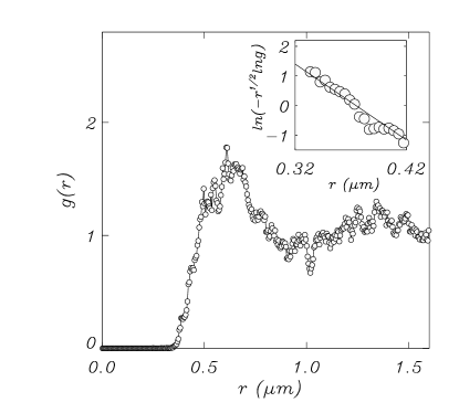
FIG. 1.: Pair correlation function obtained from averaging over Lorentz microscope images of flux lines in Nb [3, 4] at $T=5$ K. The region of interest is where $g(r)$ rises from zero (lift-off). The inset shows a comparison of the lift-off region of $g(r)$ with liquid theory behavior, Eq. (1) (refer to section II for further details).

Bitter decoration images of flux line configurations in the high temperature superconductor BSCCO analyzed in the same manner also yield results in good quantitative agreement with the accepted value of the penetration depth for BSCCO [8]. The fit value for $U_{o}$ presumably describes the characteristic energy scale for the pinscape disorder.

The present paper aims at a more thorough understanding of how structural correlations arise from microscopic properties such as the particle interactions and potential landscape. Particular questions we address include: Under what conditions can the static configurations of an interacting system in a quenched random potential give rise to liquid-like correlations of the form Eq. (1)? How does Eq. (1) compare to a theory where the quenched nature of randomness is accounted for explicitly?

We report the results of numerical simulations and present a theory that captures the essential features observed both in experiments and in our simulations, providing thus some answers to the questions raised above. In particular our simulations show that a relation of the form Eq. (1) emerges in the limit of point-like pins, i.e. pins of small spatial extent, and for broad (e.g. exponential) pinning strength distributions. In contrast, pinscapes composed of identically strong or spatially extended pins are not well described by Eq. (1). Our theory is based on the observation that the behavior of the pair correlation function at small $r$ is dominated by strongly pinned flux lines. In the low-density limit, the functional form of the pair correlation function therefore arises essentially from a convolution of the tails of the pinning energy distribution with the probability distribution for locating a flux line at a given position.

The paper is organized as follows. We present our model and its motivation in Section II. Section III contains details of the numerical simulations. Numerical results and their discussion are given in Section IV, while Section V is devoted to a description of the underlying theoretical picture. We conclude with a discussion and summary of our results in Section VI.

II The Model

We consider a two-dimensional system of $N$ particles in a quenched random pinscape consisting of discrete pinning sites positioned at random. The particles, which can be interpreted as stiff magnetic flux lines, have positions that are specified by (two-dimensional) vectors ${\bf r}_{i}$. As a convention, particle and pinning site locations are subscripted with Latin and Greek indices, respectively. The force on the $i^{th}$ flux line at position ${\bf r}_{i}$ is given by

$${\bf F}_{i}=-\sum_{j\neq i}^{N}{\bf\nabla}_{i}U({\bf r}_{i}-{\bf r}_{j})-\sum_{\alpha}{\bf\nabla}_{i}V_{\alpha}({\bf r}_{i}-{\bf r}_{\alpha}).$$ (3)

Here the first and second sum are the contributions to the total force on a given particle due to its interactions with the other particles and with the pinning sites; $U(r)$ is the interparticle interaction, whereas $V_{\alpha}(r)$ is the particle- pin interaction. For stiff magnetic flux lines, the interparticle potential $U(r)$ (per unit length) is given in the low-density limit by the asymptotic form Eq. (2). We assume that the pinning potential due to a single pin is attractive and short ranged,

$$V_{\alpha}(r)=-V_{\alpha}e^{-r^{2}/r_{p}^{2}},$$ (4)

where $V_{\alpha}$ is the pin’s strength, and $r_{p}$ its range.

The locations of the pinning sites ${\bf r}_{\alpha}$ are assumed to be distributed at random. We seek stable and static flux line configurations $\{{\bf r}^{*}_{i}\}$ given by solutions to

$${\bf F}_{i}({\bf r}^{*}_{1},{\bf r}^{*}_{2},\ldots,{\bf r}^{*}_{N})={\bf 0},$$ (5)

with the additional stability constraint that the matrix $-\partial{{\bf F}_{i}}/\partial{{\bf r}^{*}_{j}}$ be positive-definite. If $\{{\bf r}^{*}_{1},{\bf r}^{*}_{2},\ldots,{\bf r}^{*}_{N}\}$ is such a configuration, the pair correlation function $g^{*}(r)$ for this configuration is given by

$$g^{*}(r)=\frac{\langle\int\rho^{*}({\bf x}-{\bf r})\rho^{*}({\bf x})\,d{\bf x}\rangle_{\theta}}{[\int\rho^{*}({\bf x})\,d{\bf x}]^{2}},$$ (6)

with

$$\rho^{*}({\bf x})=\sum_{i=1}^{N}\delta({\bf x}-{\bf r}^{*}_{i}),$$ (7)

and $\langle\ldots\rangle_{\theta}$ denoting an average over angles. The pair correlation function $g(r)$ is obtained by averaging Eq. (6) over independent configurations.

If the analogy to liquid structure theory adequately describes the emergence of structure in this quenched random system, then Eqs. (1) and (2) imply that (to lowest order)

$$\ln(-r^{\frac{1}{2}}\ln g(r))\propto-\frac{r}{\lambda}.$$ (8)

Thus liquid theory predicts that a plot of the corresponding quantity versus $r$ should yield a linear relation with slope $1/\lambda$, as observed experimentally in the inset to Fig. 1.

Our numerical work involves solving Eq. (5) for static configurations and thereby obtaining the configuration-averaged pair correlation function. Details of the implementation and presentation of our numerical results are given in the following two sections.

III Numerical Implementation

In this section we describe our numerical implementation. Simulations were carried out on a square region with $7250$ randomly placed pins. Having constructed a random pinscape, we placed $N=65$ flux lines at random and solved numerically for stable equilibrium configurations of Eq. (5) using a three stage procedure: (i) Starting from a random initial configuration, the vortex system is allowed to relax dynamically according to

$$\frac{d{\bf{r}}_{i}}{dt}={\bf F}_{i}({\bf r}_{1},{\bf r}_{2},\ldots,{\bf r}_{N}),$$ (9)

until the magnitudes of all forces on the RHS are less than a prescribed target value. (ii) Once this has been achieved, the resulting configuration is used as an initial guess in a Newton-Raphson algorithm to find a solution to Eq. (5). Solutions found this way are not guaranteed to be stable with respect to small perturbations of the particle locations. Therefore, (iii), a linear stability analysis is carried out to check for stability. If the configuration obtained this way does not turn out to be stable, stage (i) is resumed with a reduced target value. The whole procedure is repeated until a stable configuration has been found. The combination of a molecular dynamics algorithm with a Newton-Raphson scheme, as described above, turns out to be far more computationally efficient than using molecular dynamics alone [9].

Lengths were chosen so that the square corresponds to a $5\times 5~{}\mu$m² field of view in a magnetic field of roughly $50$ Gauss. With this choice, all lengths will be reported in $\mu$m. The London penetration depth was taken to be $\lambda=0.04~{}{\mu}$m. These choices resemble the experimental condition in Ref. [3]. The parameters varied in the simulations were the range of the pinning forces $r_{p}$, with values $r_{p}\in[0.015,0.05]~{}\mu$m, and the distribution of pinning strengths $V_{\alpha}$, cf. Eq. (4). We considered the following distributions:

$${\cal P}(V_{\alpha})=\delta(V_{\alpha}-V_{o}),$$ (10)

for identical pinning strengths, and

$${\cal P}_{\nu}(V_{\alpha})=\frac{c_{1}}{V_{o}}e^{-(c_{2}\frac{V_{\alpha}}{V_{o}})^{\nu}},V_{\alpha}>0,$$ (11)

for stretched-exponentially distributed pinning strengths, with the constants $c_{1}$ and $c_{2}$ given by $c_{1}=\nu c_{2}/\Gamma(1/\nu)$, and $c_{2}=\frac{\Gamma(2/\nu)}{\Gamma(1/\nu)}$, where $\Gamma(x)$ is the Gamma function. In particular, the distributions used were $\nu=2$ (half-gaussian), $\nu=1$ (exponential), and $\nu=1/2$ (stretched exponential). The mean of the above distributions is given by $V_{o}$. The unit of energy was chosen such that

$$\frac{{\phi_{o}}^{2}r_{p}}{8\pi^{2}\lambda^{2}V_{o}}=200.$$ (12)

This choice is consistent with experimental observations [3], and ensures that the maximum force exerted by a pin is independent of the range of the pinning potential.

The numerical integration in stage (i) was carried out using a $4^{th}$ order Runge-Kutta method [10] with adaptive stepsize and an initial force resolution of $10^{-6}$ in the above units with subsequent decrements by factors of 10, as needed. Algorithms of the software libraries LINPACK and EISPACK [11] were used in putting together stages (ii) and (iii). The maximum residual force on any particle in a stable configuration was found to be smaller than $\Delta F={\cal O}(10^{-12})$.

Free boundary conditions were employed, and flux lines leaving the square (leaks) were put back in random locations. Typically, only a few leaks occurred in a given run.

In order to speed up computations further, several additional measures were taken: If a stable configuration was not found after a fixed number of integration steps $(5000)$, a new initial configuration was generated. Initial configurations were such that flux lines were randomly positioned, but no two were allowed to be closer initially than $0.2~{}\mu$m. These measures were found to reduce the computation time without changing the results significantly. The particle-pin interaction, Eq. (4), was cut off at a distance of $4r_{p}$. Prior to each run, the area was subdivided into a mesh of squares and a look-up table was generated providing each square with the location and strength of pins within the effective interaction distance $4r_{p}$. This eliminates the need to search all pinning sites for each computation of the pinning forces.

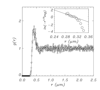
FIG. 2.: Pair correlation function $g(r)$ obtained from averaging over $212$ stable flux line configurations on a pinscape, for $\lambda=0.04$ and $r_{p}=0.015$. The pinning strengths are exponentially distributed. The inset shows a comparison with the liquid theory prediction, Eq. (8).

IV Numerical Results

In this section we present the results of our simulations described above. Fig. 2 shows the scaling of the pair correlation function obtained from averaging over $212$ stable flux line configurations on a pinscape generated with exponentially distributed pinning strengths according to Eq. (11), with $r_{p}=0.015$. The inset to Fig. 2 shows the scaling behavior of $\ln(-r^{\frac{1}{2}}\ln g(r))$ with $r$. The solid line has slope $1/\lambda$. Note the good agreement with the liquid theory prediction, Eq. (8), for values of $r$ in the initial lift-off of $g(r)$. The deviations for larger $r$ arise from excess correlations (pile-up) near the peak of $g(r)$ not accounted for in the naïve scaling Ansatz. Such excess correlations also are seen experimentally [3, 8].

Having thus observed numerically a liquid-like relation of the form Eq. (8), we next ask how the behavior of the pair correlation function depends on the range of the pinning potential $r_{p}$. Fig. 3 shows the scaling of $\ln(-r^{\frac{1}{2}}\ln g(r))$ with $r$ for different values of $r_{p}$, ranging from $0.015~{}\mu$m to $0.05~{}\mu$m.

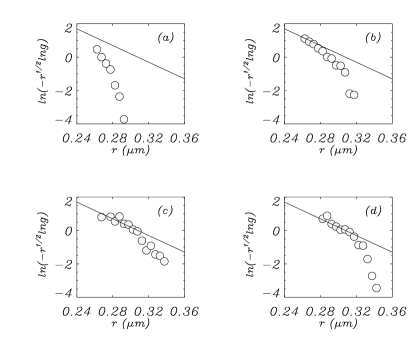
FIG. 3.: Dependence of the pair correlation function on the range of the pinning potential $r_{p}$ for exponentially distributed pinning strengths. Solid lines correspond to a liquid theory scaling, Eq.  (8), with $\lambda=0.04~{}\mu$m. The values for $r_{p}$ are $0.05~{}\mu$m (a), $0.025~{}\mu$m (b), $0.017~{}\mu$m (c), and $0.015~{}\mu$m (d). Averages were calculated from $596$, $600$, $323$ and $212$ configurations, respectively.

The asymptotic form, Eq. (8), is realized only in the limit of a short-ranged pinning potential ($r_{p}\ll\lambda$).

The dependence of the pair correlation function on the breadth of the pinning strength distribution is shown in Fig. 4. Here we compare the results for configurations on a pinscape of spatially narrow pins whose strengths were drawn from increasingly broad distributions: delta function [Eq. (10)], $\nu=2$, $1$ and $1/2$ [Eq. (11)].

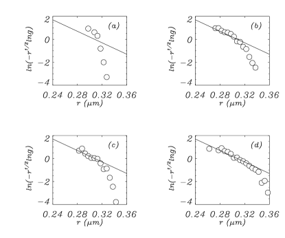
FIG. 4.: Dependence of the pair correlation function on the distribution of pinning strengths: (a) identical pinning strengths, (b) half-gaussian, $\nu=2$, (c) exponential, $\nu=1$, and (d) stretched exponential, $\nu=1/2$. Solid lines indicate the scaling, Eq. (8), for $\lambda=0.04$ ($r_{p}=0.015$). Averages were obtained from $148$, $228$, $212$, and $152$ configurations, respectively.

The pair correlation functions corresponding to the three broad distributions, $\nu=2$, $1$ and $1/2$ agree with the prediction of the liquid-like theory, Eq. (1), at least for small $r$. In contrast, Eq. (1) does not describe the case of identical pinning strengths; the rapid fall-off of $\ln(-r^{\frac{1}{2}}\ln g(r))$ indicates a steeper than expected lift-off of $g(r)$.

Thus the results of our numerical simulations clearly show a liquid-like behavior of the form Eq. (8) as observed in experiments. Furthermore our simulations indicate that this scaling only arises in the limit of point-like pins drawn from a broad distribution of pinning strengths. Its successful application to experimental data suggests that the pinscape in these materials also is characterized by point-like pins with a broad distribution of strengths. Moreover, these observations serve as a warning that simulation results based on identical pinning strengths may differ subtly from the behavior of physical systems.

V Theoretical Description

The analogy drawn between pinned flux lines and thermally disordered fluids yields an empirically satisfactory description of flux line pair correlations. To this point, though, it has been justified by heuristic arguments. This section introduces a statistical treatment of structure in strongly pinned flux lines which provides a superior description of disordered flux line distributions yet yields the liquid structure result, Eq. (1), as a limiting case.

We begin by assuming that the dominant contribution to the force on a given flux line is due to its nearest neighbor. Because of the short-range nature of the flux line interactions, this assumption is justified in the limit of low flux line concentration, where the average flux line separation, as well as fluctuations around it, are much larger than the London penetration depth. Furthermore, our simulations reveal that more than $99\%$ of the flux lines in a stable configuration are pinned, i.e. within a distance of $r_{p}/\sqrt{2}$ of a pinning site. Thus assuming that the flux lines are pinned in pairs is reasonable. In particular, this approximation is valid for pairs of flux lines pinned at distances smaller than average. These pairs determine the behavior of the pair correlation function near lift-off, i.e. the region where the function rises from zero. They occur only if sufficiently strong pins are available. In other words, a pair of nearest-neighbor flux lines can be pinned at a separation $r$ only if both pins are strong enough to overcome the flux line repulsion force, $f(r)=-\partial U(r)/\partial r$.

From Eq. (4) we see that a pin $\alpha$ of strength $V_{\alpha}$ can exert a maximum force given by

$$F_{\alpha}=\sqrt{\frac{2}{e}}\>\frac{V_{\alpha}}{r_{p}}.$$ (13)

Let $P_{d}(F_{\alpha})$ be the probability that a flux line has come to rest on a pin of maximal pinning force $F_{\alpha}$. The cumulative probability

$$Q_{d}(F)=\int_{F}^{\infty}P_{d}(F_{\alpha})dF_{\alpha}.$$ (14)

is the likelihood that the occupied pin is at least as strong as $F$. If we assume that flux lines are equally likely to be pinned anywhere in the sample as long as the corresponding pinning forces are large enough to overcome the flux line interaction, it follows that the pair correlation function $g(r)$ has the form

$$g(r)={Q_{d}}^{2}(f(r))+\ldots.$$ (15)

This expression should be valid in the low-density limit, where only pairwise-pinned flux lines have to be considered and screening effects due to the presence of other flux line pairs can be neglected. One can readily show that the resulting flux line configurations are stable.

The distribution of dynamically selected pinning strengths, $P_{d}(F_{\alpha})$, does not coincide with the corresponding distribution of a priori available strengths, $P(F_{\alpha})$. The latter is readily obtained from the pinning energy distribution, ${\cal P}_{\nu}(V_{\alpha})$, using Eq. (13). Fig. 5 compares the distributions of dynamically selected and available maximal pinning forces for exponentially distributed ($\nu=1$) pinning strengths, Eq. (11).

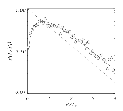
FIG. 5.: Distribution of available and dynamically selected maximal pinning forces. Shown here is the case of exponentially distributed pinning strengths, $\nu=1$. The dashed line corresponds to the distribution of available maximal pinning forces as obtained from Eqs. (13) and (11). Data points correspond to the distribution obtained by determining the pinning strength of the pins associated with every pinned flux line. The solid line corresponds to Eq. (20), as explained in the text.

We see clearly that the particles preferentially occupy strong pins. This is consistent with our expectation that an isolated flux line, or one that is effectively isolated, is more likely to be in the domain of attraction of a strong pin in its vicinity.

On the basis of this observation, we hypothesize that a given flux line dynamically selects the strongest of $n$ pins in its immediate vicinity so that

$$Q_{d}(F)=1-\left[1-Q(F)\right]^{n},$$ (16)

and thus

$$P_{d}(F)=nP(F)\left[\int_{0}^{F}P(F^{\prime})dF^{\prime}\right]^{n-1}.$$ (17)

Equations (15) – (17) and their successful application to our simulations are the central results of this article.

Fig. 5 shows that $P_{d}(F)$ is very well approximated by $n=2$, i.e.,

$$P_{d}(F)=2P(F)\int_{0}^{F}P(F^{\prime})dF^{\prime},$$ (18)

implying that its cumulative distribution $Q_{d}(F)$ obeys,

$$Q_{d}(F)=1-\left[1-Q(F)\right]^{2}.$$ (19)

We find that $n=2$ also satisfactorily describes dynamically selected pinning in our simulations with half-gaussian and stretched exponentially distributed pinning strengths, $\nu=2$ and $\nu=1/2$.

For exponentially distributed pinning strengths, $\nu=1$, we obtain

$$P_{d}(F)=\frac{2}{F_{o}}e^{-F/F_{o}}\left(1-e^{-F/F_{o}}\right),$$ (20)

where $F_{o}=\sqrt{2/e}\>V_{o}/r_{p}$. Thus,

$$Q_{d}(F)=2e^{-F/F_{o}}\left(1-\frac{1}{2}e^{-F/F_{o}}\right),$$ (21)

and, using Eq. (15),

$$g(r)=4e^{-2f(r)/F_{o}}\left[1-\frac{1}{2}e^{-f(r)/F_{o}}\right]^{2}+\ldots.$$ (22)

Analogous predictions can be obtained for the cases $\nu=2$ and $\nu=1/2$.

Fig. 6 shows comparisons of the theoretically predicted scaling of $\ln(-r^{\frac{1}{2}}\ln g(r))$ with the values obtained from our simulations for $\nu=2$, $\nu=1$ and $\nu=1/2$. These comparisons involve no adjustable parameters once $n$ has been fixed (Fig. 5), since the force scale $F_{o}$ was specified for each simulation. The results for all three pinning distributions are in very good agreement with the form predicted by Eq. (15) for $g(r)$ near lift-off.

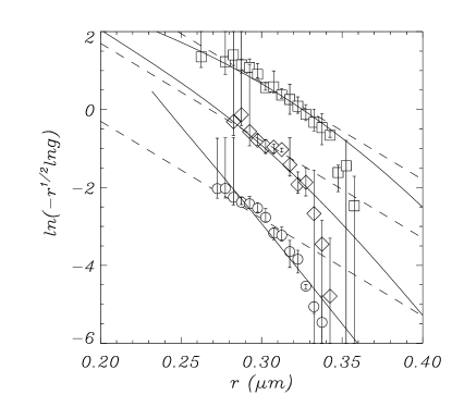
FIG. 6.: Comparison of the behavior of the pair correlation function near lift-off against simulation results, liquid theory type scaling (dashed lines) and theoretical prediction, Eqs. (15) and (19), for half-gaussian (circles), exponential (diamonds), and stretched exponential $\nu=1/2$ (boxes) distribution of pinning strengths. Note that the theoretical predictions contain no free parameter once $n$ has been fixed (Fig. 5), while the liquid theory predictions are one-parameter fits to the form Eq. (1). Curves have been vertically offset for clarity.

The relative success of the present theory compared with the liquid structure Ansatz in predicting the behavior of $g(r)$ near lift-off emphasizes fundamental differences between the two classes of systems. In thermal systems such as simple liquids, structural correlations arise from the interplay of interaction energies and the thermal energy scale. Systems such as pinned flux lines are dominated by quenched disorder and select configurations in which forces are balanced. Nevertheless, the two approaches yield comparable predictions for the flux line distribution because of the exponential form of the pair potential, Eq. (2).

Fig. 4(a) reveals that a pinscape generated by identical pins differs from the more broadly distributed cases in that it gives rise to a distinctively steep lift-off in the pair correlation function. This behavior is captured also by the present treatment. In the low-density limit, the theoretical description, Eq. (15), predicts a step-like increase in $g(r)$ for the smallest separation at which a pair of flux lines can be pinned against their mutual repulsion. Fig. 4(a) shows somewhat smoother behavior. Analyzing the configurations contributing to the lift-off of $g(r)$ shows that this smoothing is due to many-body effects, i.e. flux lines pinned by the interaction with two or more close-by flux lines. Comparing this discrepancy to the good agreement with the theoretical prediction in the case of broadly distributed pinning strengths leads us to conclude that, in these cases, the disorder due to variation in pinning strength dominates the contribution arising from the spatial disorder of the flux line configurations.

A liquid-like form for $g(r)$ can be obtained only if the distribution of dynamically selected pins is exponential. Eqs. (15) and (16) show that, in the general case, prefactors and different forms of leading order behavior can arise depending on the the tails of the (dynamical) pinning energy distribution. Our results in Fig. 6 suggest, however, that this dependence is weak and will become detectable only for very small values of $r$. This is consistent with the success of Eq. (1) in describing experimental data. We also investigated systems of particles interacting with power law potentials and found that, when the interactions fall off sufficiently fast, the pair correlation is again of the form Eq. (15).

VI Discussion and Conclusions

We have shown that the pair correlation function arising from stable configurations of interacting particles in a random pinscape can contain information about both the particle interactions and also the statistical properties of the underlying pinscape. Our analysis shows that this is the case in the regime where the pinning and pair interactions are of comparable strength. If the pinning completely dominates pair interactions, the pair correlation function will essentially reveal the spatial disorder of the active pinning sites. In the opposite limit, in which the pair interactions dominate, the pair correlation function will contain features corresponding to crystalline order. In both cases, little information can be extracted about the form of the interactions.

We have derived an expression for the pair correlation function in the limit of point-like disorder and low flux line density, Eq. (15). Our theory shows that the small $r$ behavior of the pair correlation function depends both on the pair interaction and also on the availability of strong pinning sites. We found that the distribution of the latter is not necessarily the same as the distribution of a priori available pinning sites. Rather, the dynamics favor strong pins. Inspection of the stable configurations revealed that the distribution of dynamically selected pins is consistent with a process of choosing the strongest out of $n$ available pins. For the parameters used in our simulations, $n=2$ described the dynamically selected pinning strength distributions very well. We expect however that the parameter $n$, while apparently independent of the width of the pinning strength distribution, should depend on both the concentration of pins and also the penetration depth of the flux line interaction. A more detailed investigation will be left for future work.

We now turn to a comparison of the qualitative features of the experimentally obtained pair correlation functions with those obtained from simulation. We find that the width and location of the first peak of $g(r)$ is different: while the first peak of the pair correlation function as obtained from experiments (cf. Fig. 1) is broad and occurs around the mean flux line spacing, we see a much narrower peak in our simulations (cf. Fig. 2). Moreover the first peak occurs at a distance significantly smaller than the mean flux line spacing. Thus the numerical simulations have larger fluctuations in the local flux line density than are seen in experiment. A reason for this is that our particle-like treatment of flux lines ignores their magnetic properties. One expects that including boundary conditions for a uniform applied external magnetic field would favor a homogeneous flux line concentration and thus would penalize the large fluctuations in our simulations.

We thank Gene Mazenko for enlightening discussions. This work was supported in part by the National Science Foundation through the Science and Technology Center for Superconductivity under Award Number DMR-9120000 and in part by the MRSEC program of the National Science Foundation under Award Number DMR-9400379. C. H. S. would like to acknowledge the support of the National University of Singapore. M. M. acknowledges partial support from the Kerpişçi Foundation.

REFERENCES

- [1] G. Blatter, M. V. Feigel’man, V. B. Geshkenbein, A. I. Larkin, and V. M. Vinokur, Rev. Mod. Phys. 66, 1125 (1994).
- [2] See for example: G. Grüner, Rev. Mod. Phys. 60, 1129 (1988); E. Y. Andrei, G. Deville, D. C. Glattli, F. I. B. Williams, E. Paris and B. Etienne, Phys. Rev. Lett. 60, 2765 (1988); R. L. Willett, in Phase Transitions and Relaxations in System with Competing Energy Scales, T. Riste and D. Sherrington, eds., Nato ASI series vol. 415, p. 367 (Kluwer Academic Pub., Dordrecht, 1993) and references therein; L. V. Mikheev, B. Drossel and M. Kardar, Phys. Rev. Lett. 75, 1170 (1995); L. Balents, M. C. Marchetti and L. Radzihovsky, Phys. Rev. B 57, 7705 (1998); S. Scheidl and V. M. Vinokur, Phys. Rev. E 57, 2574 (1998).
- [3] C.H. Sow et al., Phys. Rev. Lett. 80, 2693 (1998).
- [4] K. Harada et al., Science 274, 1167 (1996).
- [5] J.- P. Hansen and I. R. McDonald, Theory of simple Liquids, (Academic Press, London, 1986), 2nd ed.
- [6] P. G. de Gennes, Superconductivity of Metals and Alloys, (Benjamin, New York, 1966).
- [7] M. Abramovitz and I. A. Stegun, Handbook of Mathematical Functions, (Dover, New York, 1972).
- [8] C.H. Sow et al., in preparation.
- [9] A similar algorithm was used in A. A. Middleton and D. S. Fisher, Phys. Rev. B 47, 3530 (1993).
- [10] W. H. Press, B. P. Flannery, S. A. Teukolsky and W. T. Vetterling, Numerical Recipes, The Art of Scientific Computing, (Cambridge University Press, Cambridge, 1989).
-
[11]
The algorithms of the LINPACK and EISPACK software libraries
can be found for example at:
http://www.netlib.org/