Formation of electron-hole pairs in a one-dimensional random environment

Abstract

We study the formation of electron-hole pairs for disordered systems in the limit of weak electron-hole interactions. We find that both attractive and repulsive interactions lead to electron-hole pair states with large localization length $\lambda_{2}$ even when we are in this non-excitonic limit. Using a numerical decimation method to calculate the decay of the Green function along the diagonal of finite samples, we investigate the dependence of $\lambda_{2}(U)$ on disorder, interaction strength $U$ and system size. Infinite sample size estimates $\xi_{2}(U)$ are obtained by finite-size scaling. The results show a great similarity to the problem of two interacting electrons in the same random one-dimensional potential.

It is well-known that randomness leads to localization of non-interacting electrons and holes. This effect is especially strong in one-dimensional (1D) systems [1, 2] leading to complete localization even for very small disorder [3]. On the other hand, in the limit of strong attractive Coulomb interaction, electrons and holes will pair into excitons with large lifetimes. In the present work, we concentrate on the intermediate problem of weakly interacting electrons and holes (IEH) in a random environment. The energy scales are such that the band width is larger than the disorder $W$ which in turn is larger than the interaction strength $U$ and so we do not have bound excitons, but rather electron-hole pairs. Such a problem is relevant for the proposed experimental verification of the two-interacting particle (TIP) effect by optical experiments in semiconductors [4]. The TIP problem has recently attracted a lot of attention after Shepelyansky [5, 6] argued that attractive as well as repulsive onsite interactions between two bosons or fermions in a single random potential lead to the formation of particle pairs whose localization length $\lambda_{2}\propto U^{2}\lambda_{1}^{2}$ is much larger than the single-particle (SP) localization length $\lambda_{1}$. His major prediction is that in the limit of weak disorder a pair of particles will travel much further than a SP even for repulsive interaction $U>0$.

Here, we consider the effect of onsite interaction on a single electron-hole pair, modelled by TIP in two different 1D random potentials. The Hamiltonian we consider is

$$H = -t\sum_{n,m}\left(|n,m\rangle\langle n+1,m|+|n,m\rangle\langle n,m+1|+h.c.\right)$$ (2)

$$\mbox{ }+\sum_{n,m}|n,m\rangle\left(\epsilon^{1}_{n}+\epsilon^{2}_{m}+U\delta_{nm}\right)\langle n,m|$$

where for the case of TIP in different potentials, e.g. two electrons on neighboring chains, or an electron and a hole on the same chain, we have $\epsilon^{1}_{n}\neq\epsilon^{2}_{n}$. For simplicity, both $\epsilon^{1}_{n}$ and $\epsilon^{2}_{n}$ are chosen randomly from the interval $[-W/2,W/2]$. In the following we call this situation the IEH case. We will show that the results for IEH are similar to the (standard) TIP problem when both particles are in the same potential $\epsilon^{1}_{n}=\epsilon^{2}_{n}$. In both cases $U$ is the on-site interaction between the two particles. We use hard-wall boundary conditions and the hopping element $t\equiv 1$ sets the energy scale. We note that this Hamiltonian corresponds to the 2D Anderson model if we replace $\epsilon^{1}_{n}+\epsilon^{2}_{m}$ in (2) by $\tilde{\epsilon}_{nm}$ and choose $\tilde{\epsilon}_{nm}\in[-W/2,W/2]$. In this case $U$ is an added on-site potential. This has been recently used to test our numerical method by comparing with more established methods valid for this model [7].

To obtain our results we use a decimation method (DM) [7, 8]. This involves replacing the full Hamiltonian by an effective Hamiltonian for the doubly-occupied sites only. It should be stressed that this method is exact and no approximations have to be made in the decimation process. It is then possible, via a simple inversion, to obtain the Green function matrix elements $\langle 1,1|{G_{2}}|M,M\rangle$ between doubly-occupied sites. We shall be focusing on the IEH localization length $\lambda_{2}$ obtained from the decay of the transmission probability of IEH from one end of the system to the other. This is defined [9] by

$${1\over\lambda_{2}}=-{1\over|M-1|}\ln|\langle 1,1|{G_{2}}|M,M\rangle|.$$ (3)

In order to reduce possible boundary effects, we compute $\lambda_{2}$ by considering the decay between sites slightly inside the sample. We present results for the band centre, i.e., energy $E=0$ for $14$ disorder values $W$ between $0.5$ and $7$, for 21 system sizes $M$ between $51$ and $251$, and 11 interactions strengths $U=0,0.1,\ldots,1.0$. For each triplet of parameters $(W,M,U)$ we average the localization lengths $\lambda_{2}$ computed from the Green function according to Eq. (3) over 100 samples.

In Fig. 1, we show the IEH results for $M=201$. Let us first turn our attention to the case $U=0$. As pointed out previously [10], the TIP Green function ${G_{2}}$ at $E=0$ is given by a convolution of two SP Green functions ${G_{1}}$ at energies $E_{1}$ and $-E_{1}$. This implies that $\lambda_{2}\approx\lambda_{1}/2$. We have therefore included data for $\lambda_{1}/2$ in Fig. 1 which we have computed by a transfer matrix method (TMM) [11] in 1D with $0.1\%$ accuracy. Comparing these results to the localization lengths $\lambda_{2}$ obtained from the DM, we find that for $1\leq W\leq 6$, the agreement between $\lambda_{2}(U=0)$ and $\lambda_{1}/2$ is rather good and, contrary to TMM results [12, 13, 14], there is no large artificial enhancement at $U=0$. For smaller disorders $W<1$, we have $\lambda_{2}\approx M/2$ so that it is not surprising that the Green function becomes altered due to the finiteness of the chains [15]. This results in reduced values of $\lambda_{2}$. It is noticeable from these results, however, that the values of $\lambda_{2}(U=0)$ are still slightly larger than $\lambda_{1}/2$. This is similar to TIP results [10] and to a numerical convolution of the SP Green functions calculated by exact diagonalisation [7]. For $U$ between $0.1$ and $1$ and $W\geq 1.2$ we have found that the localization lengths $\lambda_{2}(U)$ are increased by the onsite interaction as shown in Fig. 1. For $U\gg 1$, it is well-known that the interaction will split the single TIP band into upper and lower Hubbard bands and, hence, we expect that for large $U$ the enhancement of the localization length at $E=0$ will vanish. In Fig. 2 we present data for $\lambda_{2}(U)/\lambda_{2}(0)$ for $U=-4,\ldots,4$. We first observe that at the band centre the enhancement is symmetric in $U$. This is why we usually only consider $U>0$ in agreement with the previous arguments and calculations for the TIP case [7, 9, 10, 12, 13, 14, 15, 16, 17]. We have checked that away from the band centre the enhancement is asymmetric in $U$. For small $|U|$, we see from Fig. 2 that the localization length increases nearly linearly in $|U|$ with a slope that is larger for smaller $W$ and we do not see any $U^{2}$ behavior as argued in Refs. [5, 6, 18]. At large $|U|$ the enhancement starts to decrease again. For TIP, it has been suggested [17] that there exists a duality for $U$ and $\sqrt{24}/U$ for very large $|U|$. The crossover between the two asymptotic regimes should accor at $U_{c}=24^{1/4}$. For IEH, we find that within the accuracy of our data, we can argue for an agreement with the duality. As for our TIP data [7], we observe the best IEH agreement with duality for $W=5$ but the maximum enhancement $\max_{U}\left[\lambda_{2}(U)/\lambda_{2}(0)\right]$ still seems to depend upon the disorder.

In order to overcome the problems with the finite chain lengths, we construct finite-size scaling (FSS) curves for each $U$ and compute from these scaling parameters which are the infinite-sample localization lengths $\xi_{2}(U)$. This method has been proven very useful for the non-interacting case [19] and recently for TIP studies [7, 10]. In Fig. 3 we show the raw data of the reduced IEH localization lengths $\lambda_{2}/M$ which are to be scaled just as in the standard TMM [19]. Note that data for small $W$ are rather noisy and will thus most likely not give very accurate scaling. In order to set an absolute scale in the FSS procedure, one usually fits the smallest localization lengths of the largest systems to $\lambda_{2}/M=\xi_{2}/M+b(\xi_{2}/M)^{2}$ with $b$ small [19]. Due to numerical problems of estimating a small localization length of the order of $1$ in a large system by Eq. (3) we instead fit for each $U$ to the localization length at $W=3$ and adjust the absolute scale of $\xi_{2}$ accordingly. In Fig. 4 we show the resulting scaling curves $\lambda_{2}/M=f(\xi_{2}/M)$ for $U=0$, $0.2$ and $1$. The above mentioned numerical errors in the data at large $M$ and $W$ are visible only in very small upward deviations from the expected $1/M$ behavior. The results are very similar to the TIP problem. It is interesting to note that it is even possible to scale the present IEH data together with the data previously obtained for the TIP case [7]. From this more accurate scaling we compute the scaling parameters $\xi_{2}$ which we show in Fig. 5. The power-law fits $\xi_{2}\propto W^{-2\alpha}$ to the data with $W\in[1,5]$ yield an exponent $\alpha$ which increases with increasing $U$ as shown in the inset of Fig. 5, e.g., $\alpha\approx 1.1$ for $U=0$ and $\alpha\approx 1.5$ for $U=1$. Thus, although in Fig. 1 the $\lambda_{2}$ data at $M=201$ nicely follows $\lambda_{1}/2$ for $U=0$, we nevertheless find that after FSS with data from all system sizes, $\xi_{2}(0)$ as against $\lambda_{1}/2$ still gives a slight enhancement. Because of this we will in the following compare $\xi_{2}(U>0)$ with $\xi_{2}(0)$ when trying to identify an enhancement of the localization lengths due to interaction. For comparison, the exponents obtained from the same fit applied to the TIP problem [7] are also shown. Note that, as expected from Fig. 3, FSS is not very accurate for small $W$. Therefore, in what follows we shall only use $\xi_{2}$ values obtained for $W\geq 1$. For data corresponding to $W<1$, we actually used the extrapolated values of $\xi_{2}$ from the power-law fit to continue the FSS curves of Fig. 4 to $W<1$.

We now compare our IEH results with various fits proposed for TIP. From an effective random matrix model [5, 15, 16] $\lambda_{2}\,\propto\,\lambda_{1}^{\beta}$ was obtained for large values of $\lambda_{1}$. To correct for smaller values of $\lambda_{1}$ a more accurate expression was suggested [16] to be $\lambda_{2}\,\propto\,\lambda_{1}^{\beta}(1+c/\lambda_{1})$. It is important that $\beta$ in this work depends on $U$ and ranges from $1$ at small $U$ and very large $U$ to nearly $2$ for $U\approx t$. As discussed above we translate this fit function into $\xi_{2}(U)\propto\xi_{2}(0)^{\beta}\left(1+\frac{c}{\xi_{2}(0)}\right)$. In Fig. 6 we show respective data for disorders $W\in[1,6]$. The fits are good and reflect in particular the deviations from a simple power-law $\xi_{2}(U)\propto\xi_{2}(0)^{\beta}$ for small localization lengths. In the inset we present the dependence of $\beta$ on $U$: we find $\beta<1.5$ for all $U$ values considered unlike Ref. [16]. The values obtained for the TIP case [7] are shown for comparison.

In Ref. [9] the functional dependence of the TIP localization lengths $\lambda_{2}=\lambda_{1}/2+c|U|\lambda_{1}^{2}$ has been suggested. Taking instead of $\lambda_{1}/2$ the more suitable $\xi_{2}(0)$ this can be translated as $\xi_{2}(U)-\xi_{2}(0)\propto|U|\xi_{2}(0)^{2}$. In Fig. 7 we plot $[\xi_{2}(U)-\xi_{2}(0)]/|U|$ vs. $g(U)\xi_{2}(0)$ for $U\in[0.1,1]$ where we have chosen $g(U)$ so that the data for different $U$ can be placed on top of the $U=0.1$ data. In the inset of Fig. 7 we show that $g(U)$ starts to deviate from $1$ already for $U\geq 0.4$. Thus we see that the linear behavior in $|U|$ found in Ref. [9] holds only for very small $U$ in agreement with TIP. We obtain a good fit to $[\xi_{2}(U)-\xi_{2}(0)]/|U|$ with a single exponent $\beta=1.6\pm 0.1$ instead of $2$. This is somewhat different from the fits for TIP which give $\beta\approx 2$ for small $\xi_{2}(0)<10$ and $\beta\approx 3/2$ for larger $\xi_{2}(0)$ [7]. The reduction of the slope below $\beta=2$ may be due to insufficient disorder averaging and thus an underestimation of the FSS results.

In conclusion, we have presented detailed results for the localization lengths of electron-hole pair states which may be realized in the non-excitonic limit of optically excited semiconductor heterostructures [4]. We observe an increase of the two-particle localization length due to onsite interaction in the band centre. This suggests the formation of an electron-hole pair with possibly enhanced transport properties. We emphasize that our results apply to the non-excitonic limit with bandwidth larger than $W>U$. We have fitted our data to various suggested models with varying success. The results are all similar to the standard TIP problem in a single random potential and thus we conclude that the case of an interacting electron-hole pair is very close to the TIP problem [7].

We thank E. McCann, J. E. Golub, O. Halfpap and D. Weinmann for useful discussions. R.A.R. gratefully acknowledges support by the Deutsche Forschungsgemeinschaft through SFB 393.

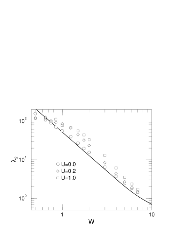
FIG. 1.: Localization length $\lambda_{2}$ at energy $E=0$ for system size $M=201$ and different interaction strengths. The thick solid line represents data for $\lambda_{1}/2$.

FIG. 2.: Enhancement $\lambda_{2}(U)/\lambda_{2}(0)$ as a function of interaction strength $U$ at $E=0$ for disorder $W=3$ ($+$), $4$ ($*$), and $5$ ($\times$) and $M=201$. The thick (thin) lines indicate data for $U>0$ ($U<0$), full (open) circles denote the maximum for each disorder. The dashed line marks $U_{c}=24^{1/4}$.

FIG. 3.: Reduced localization lengths $\lambda_{2}/M$ for $U=0$ (left) and $U=1$ (right) for $14$ disorders between $0.5$ (A) and $7$ (N) as in Fig. 1.

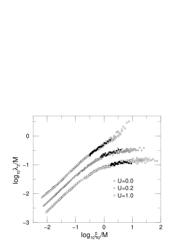
FIG. 4.: Finite-size scaling plot of the reduced localization lengths $\lambda_{2}/M$ for various $U$. The data for $U=0.2$ ($1$) have been divided by 2 (4) for clarity. Data corresponding to $W=1$ are indicated by filled symbols.

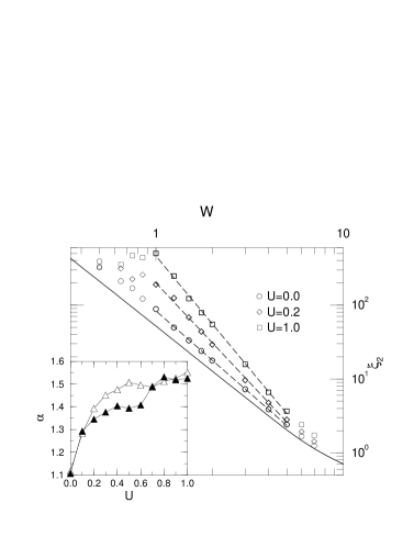
FIG. 5.: Localization lengths $\xi_{2}$ after FSS for various $U$. The solid line represents $\lambda_{1}/2$, the dashed lines indicate power-law fits. Inset: Exponent $\alpha$ obtained by fitting $\xi_{2}\propto W^{-2\alpha}$ to the data for each $U$ (filled symbols). The result for the standard TIP problem is also shown (open triangles).

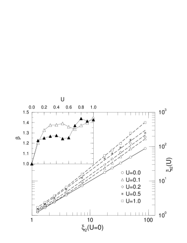
FIG. 6.: $\xi_{2}(U)$ after FSS for various $U$ plotted versus $\xi_{2}(0)$. The lines are fits $\xi_{2}(U)\propto\xi_{2}(0)^{\beta}[1+c/\xi_{2}(0)]$. Inset: Exponent $\beta$ from the fits (filled symbols) and for the standard TIP problem (open triangles).

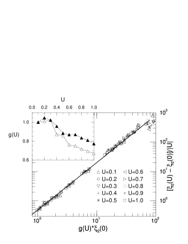
FIG. 7.: Enhancement of the localization lengths $[\xi_{2}(U)-\xi_{2}(0)]/|U|$ plotted for $W\in[1,7]$ versus $g(U)\xi_{2}(0)$ where $g(U)$ was obtained by a mean-least-squares fit procedure to make all the data compatible with $g(0.1)=1$. The straight line is the curve $\xi_{2}(U)=\xi_{2}(0)+0.49|U|[g(U)\xi_{2}(0)]^{1.61}$. Inset: Behaviour of $g(U)$ for IEH (filled symbols) and for TIP [7] (open triangles).

REFERENCES

- [1] see, e.g., P. A. Lee and T. V. Ramakrishnan, Rev. Mod. Phys. 57, 287 (1985) and D. Belitz and T. R. Kirkpatrick, Rev. Mod. Phys. 66, 261 (1994).
- [2] E. Abrahams, P. W. Anderson, D. C. Licciardello, and T. V. Ramakrishnan, Phys. Rev. Lett. 42, 673 (1979).
- [3] B. Kramer and A. MacKinnon, Rep. Prog. Phys. 56, 1469 (1993).
- [4] J. E. Golub, private communication; D. Brinkmann, J. E. Golub, S. W. Koch, P. Thomas, K. Maschke, I. Varga, preprint (1998).
- [5] D. L. Shepelyansky, Phys. Rev. Lett. 73, 2607 (1994); F. Borgonovi and D. L. Shepelyansky, Nonlinearity 8, 877 (1995); —, J. Phys. I France 6, 287 (1996).
- [6] D. L. Shepelyansky, in Correlated fermions and transport in mesoscopic systems, Eds. T. Martin, G. Montambaux, and J. Trân Thanh Vân, Editions Frontieres, Gif-sur-Yvette, p. 201 (1996) (Proc. XXXI Moriond Workshop, 1996, cond-mat/9603086).
- [7] M. Leadbeater, R.A. Römer and M. Schreiber, submitted to Eur. Phys. J. B, (1998, cond-mat/9806255).
- [8] C. J. Lambert, D. Weaire, phys. stat. sol. (b) 101, 591 (1980).
- [9] F. v. Oppen, T. Wettig, and J. Müller, Phys. Rev. Lett. 76, 491 (1996).
- [10] P. H. Song and D. Kim, Phys. Rev. B 56, 12217 (1997).
- [11] G. Czycholl, B. Kramer, and A. MacKinnon, Z. Phys. B 43, 5 (1981); J.-L. Pichard, J. Phys. C 19, 1519 (1986).
- [12] K. Frahm, A. Müller-Groeling, J.-L. Pichard, and D. Weinmann, Europhys. Lett. 31, 169 (1995).
- [13] R. A. Römer and M. Schreiber, Phys. Rev. Lett. 78, 515 (1997); D. Weinmann, A. Müller-Groeling, J.-L. Pichard, and K. Frahm, Phys. Rev. Lett. 78, 4889 (1997); R. A. Römer and M. Schreiber, Phys. Rev. Lett. 78, 4890 (1997); —, phys. stat. sol (b) 205, 275 (1998).
- [14] O. Halfpap, A. MacKinnon, and B. Kramer, to be published in Sol. State. Comm., (1998); O. Halfpap, I. Kh. Zharekeshev, B. Kramer, and A. MacKinnon, preprint (1998).
- [15] T. Vojta, R. A. Römer, and M. Schreiber, preprint (1997, cond-mat/0702241).
- [16] I. V. Ponomarev and P. G. Silvestrov, Phys. Rev. B 56, 3742 (1997).
- [17] X. Waintal, D. Weinmann, and J.-L. Pichard, preprint (1998, cond-mat/9801134).
- [18] Y. Imry, Europhys. Lett. 30, 405 (1995).
- [19] A. MacKinnon and B. Kramer, Z. Phys. B 53, 1 (1983).