June 1998

(revised) October 1998

UT-KOMABA/98-16

cond-mat/9806349

Hamiltonian cycles

on random lattices of arbitrary genus

Saburo Higuchi

Department of Pure and Applied Sciences,

The University of Tokyo

Komaba, Meguro, Tokyo 153-8902, Japan

Abstract

A Hamiltonian cycle of a graph is a closed path that visits every vertex once and only once. It has been difficult to count the number of Hamiltonian cycles on regular lattices with periodic boundary conditions, e.g. lattices on a torus, due to the presence of winding modes. In this paper, the exact number of Hamiltonian cycles on a random trivalent fat graph drawn faithfully on a torus is obtained. This result is further extended to the case of random graphs drawn on surfaces of an arbitrary genus. The conformational exponent $\gamma$ is found to depend on the genus linearly.

PACS: 05.20.-y; 02.10.Eb; 04.60.Nc; 82.35.+t

Keywords: random graph; random lattice; Hamiltonian cycle; self-avoiding walk; compact polymer

1 Introduction

Properties of Hamiltonian cycles and walks on regular and random lattices have been attracting much attention recently [1, 2, 3, 4, 5, 6]. A Hamiltonian cycle (walk) of a graph is a closed (open) path which visits every vertex once and only once, i.e., a self-avoiding loop (walk) which visits all the vertices. The system of a Hamiltonian cycle (walk) on a lattice serves as a model of compact ring (linear) polymer which fills the lattice completely [7]. It is also relevant to the protein folding problem [8, 9, 10].

Among the properties of Hamiltonian cycles, the number of Hamiltonian cycles on a given graph is one of the most fundamental and interesting quantities. The number is directly related to the entropy of a lattice polymer in the compact phase. When it is non-zero, it also coincides with the degeneracy of optimal solutions to the traveling salesman problem on the graph. The number has been calculated exactly or numerically for a number of fixed regular lattices [11, 12, 13, 14, 15, 16, 1].

In this article, I am concerned with random lattices and study the number of Hamiltonian cycles on them. Specifically, I exactly evaluate the number $F_{n}^{(g)}:=\sum_{G\in S^{n,g}}\mathcal{H}(G)/(\#\mathrm{Aut}\ G)$, where the number of Hamiltonian cycles on a given graph $G$ is denoted by $\mathcal{H}(G)$. The ensemble $S^{n,g}$ is the set of all trivalent fat graphs that have $n$ vertices and can be drawn faithfully on a surface of genus $g$ ( but not on that of $g-1$). See Fig. 1 for an example. The integer $\#\mathrm{Aut}\ G$ is related to the symmetry of $G$ and is defined precisely in section 2. This result extends those of refs. [5, 6] where only the planar case ($g=0$) has been studied.

The case $g=1$ (torus) is especially interesting in that it can be compared with the corresponding problem on a two-dimensional fixed regular lattice with the periodic boundary condition for each of the two directions [2]. This comparison provides a good illustration of nature of statistical systems on random lattices.

From the exact integral expression of $F_{n}^{(g)}$, one can extract the large-$n$ asymptotics of the ‘random average’ of $\mathcal{H}(G)$. It is found that the site entropy is independent of the genus $g$ while the conformational exponent $\gamma$ depends on it linearly. This behavior is consistent with the KPZ-DDK scaling [17, 18, 19] for two-dimensional gravity coupled to $c=-2$ conformal matter [5, 6].

The organization of the paper is as follows. I give definitions and fix notations in section 2. In section 3, the calculation for a random graph on a torus is presented, putting emphasis on the difference from the case of a fixed regular lattice on a torus. The analysis is extended to the case of surfaces of an arbitrary genus to yield a simple integral expression in section 4. I discuss my results in section 5.

2 Definitions

Definitions in this section generalize those given in ref. [6].

Let $S^{n,g}$ be the set of all trivalent fat graphs that have $n$ vertices possibly with multiple-edges and self-loops and can be drawn faithfully on an orientable surface $\Sigma_{g}$ of genus $g\geq 0$ (but not on $\Sigma_{g-1}$). An example of a trivalent fat graph is drawn in Fig 1.

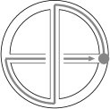
Figure 1: An example of a trivalent fat graph $G\in S^{4,1}$ which can be drawn on a torus but not on a sphere. A Hamiltonian cycle is drawn in a gray line. For this graph, $\mathcal{H}(G)=8$ because a direction (arrow) and a base point (dot) are associated with a Hamiltonian cycle.

Graphs that are isomorphic are identified. The set $\tilde{S}^{n,g}$ is the labeled version of $S^{n,g}$, namely, vertices of $\tilde{G}\in\tilde{S}^{n,g}$ are labeled $1,\ldots,n$ and $\tilde{G}_{1},\tilde{G}_{2}\in\tilde{S}^{n,g}$ are considered identical only if a graph isomorphism preserves labels. The symmetric group of degree $n$ naturally acts on $\tilde{S}^{n,g}$ by the label permutation. The stabilizer subgroup of $\tilde{G}$ is called the automorphism group $\mathrm{Aut\ }G$.

A Hamiltonian cycle of a labeled graph $\tilde{G}\in\tilde{S}^{n,g}$ is a directed closed path (consecutive distinct edges connected at vertices) which visits every vertex once and only once. Hamiltonian cycles are understood as furnished with a direction and a base point (denoted by an arrow and a dot in figures). The number of Hamiltonian cycles of $\tilde{G}$ is denoted by $\mathcal{H}(G)$ because it is independent of the way of labeling.

The quantity I study in this work is

$$F_{n}^{(g)}:=\sum_{G\in S^{n,g}}\mathcal{H}(G)\frac{1}{\#\mathrm{Aut\ }G}$$ (1)

and the generating function

$$F^{(g)}(p):=\sum_{n=0}^{\infty}p^{n}F_{n}^{(g)}.$$ (2)

The key observation made in ref. [6] has been that $F_{n}^{(0)}$ can be written as the number of isomorphism classes of the pair (graph, Hamiltonian cycle) and thus is an integer. It is also true for $F_{n}^{(g)}$ with $g>0$ :

$$F_{n}^{(g)}=\#(\{(\tilde{G},C^{n})|\tilde{G}\in\tilde{S}^{n,g},C^{n}:\text{Hamiltonian cycle on }\tilde{G}\}/\sim),$$ (3)

where $(\tilde{G}_{1},C^{n}_{1})\sim(\tilde{G}_{2},C^{n}_{2})$ if and only if $G_{1}$ and $G_{2}$ are isomorphic (forgetting the labels) and the isomorphism maps $C^{n}_{1}$ onto $C^{n}_{2}$ with the direction and the base point preserved.

3 Lattices on a torus

Before proceeding to the calculation of $F^{(1)}_{n}$, let us take a glance at the case of fixed regular lattices on a torus $\Sigma_{1}$. Given a fixed base point, a Hamiltonian cycle represents an element of the fundamental group $\pi(\Sigma_{1})\simeq\mathbb{Z}a+\mathbb{Z}b$ where $a$ and $b$ are the meridian and the longitudinal cycles. Reflecting this fact, there are many topological sectors for self-avoiding loops (thus for Hamiltonian cycles) as depicted in Fig 2.

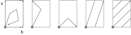
Figure 2: Examples of the ways how self-avoiding loops (gray lines) wind around tori. A torus $\Sigma_{1}$ is drawn as a rectangle with two pairs of edges identified, with the generator $a,b\in\pi_{1}(\Sigma_{1})$. From left to right, the loop represents $0,a,b,2a+b$, and $2a+3b\in\pi_{1}(\Sigma_{1})$, respectively.

More precisely, an element $m_{1}a+m_{2}b\in\pi_{1}(\Sigma_{1})$ can be represented by a self-avoiding loop if and only if the pair $(m_{1},m_{2})$ satisfies

$$(m_{1},m_{2})=(0,0),(\pm 1,0),(0,\pm 1),\quad\text{or}\quad\mathrm{gcd}[m_{1},m_{2}]=1.$$ (4)

This rich structure gives rise to an interesting question: how many Hamiltonian cycles belong to a given topological sector ? But at the same time, the existence of many topological modes is an obstacle to calculating $\mathcal{H}(G)$.

In the transfer matrix method for calculating $\mathcal{H}(G)$, one maps the system into a state sum model with a local weight. Once mapped to a state sum model, its transfer matrix can be diagonalized by employing the Bethe ansatz [14, 15] or numerical calculation [20, 16]. In the mapping, it is crucial to avoid contributions from vacuum loops, or small loops disconnected from the largest loop component in question. This non-local constraint can be imposed as follows. First one assigns directions to each loop component and makes the weight direction dependent. The sum over all the assignments is taken. Then the weight is tuned so as that the cancelation occurs between two configurations having the vacuum loop of the same shape but with the opposite directions.

This procedure is straightforward for lattices with disk topology because all vacuum loops are topologically trivial. In the case of cylinder geometry, vacuum loops winding around the cylinder should be taken care of. To make the cancelation work, one introduces the ‘seam’ and associates additional weights to vacuum loops going across the seam and winding around the cylinder.

When one further imposes periodicity to the other direction to have a torus, one come to have a huge number of topologically inequivalent vacuum loops as shown in Fig. 2. As far as the present author knows, there is no simple way to avoid a contribution from each of these vacuum loops in the transfer matrix method. Thus, for fixed lattices on a torus, one has to employ the direct enumeration or the field theoretic approximation in order to evaluate $\mathcal{H}(G)$ [2].

Note that the Coulomb gas method [4, 1, 3], which is capable of determining exact critical exponents, again works for the disk or cylinder topology but not for the torus topology .

For random lattices, however, the situation changes dramatically. Changing the order of the summation, I shall sum over random lattice structures first fixing the topological sector of the Hamiltonian cycle. Then I sum over the topological sectors. Because the summation is performed over random lattices, there is no preferred basis $\langle a,b\rangle$. One is free to perform a modular transformation on a torus to map $m_{1}a+m_{2}b\mapsto 1\cdot a,b\mapsto b$ if $m_{1}\neq 0$ or $m_{2}\neq 0$. In other words, only two topological classes of cycles are distinguishable: the non-winding sector ($m_{1}=m_{2}=0$) and the winding sector ($m_{1}\neq 0$ or $m_{2}\neq 0$). A contribution from each sector is denoted by $F^{(1),0}_{n}$ and $F^{(1),1}_{n}$, respectively (Fig 3)

$$F^{(1)}_{n}=F^{(1),0}_{n}+F^{(1),1}_{n},\ \ F^{(1),w}(p):=\sum_{n=0}^{\infty}p^{n}F^{(1),w}_{n}.$$ (5)

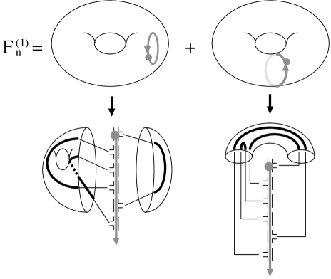
Figure 3: Configurations contributing to each of two topological sectors (left: $F^{(1),0}_{6}$, right: $F^{(1),1}_{6}$). The sequence of T’s in the center is obtained by walking along the Hamiltonian cycle (the gray line in the T’s). The vertical segments of T’s on both sides should be connected by black fat lines on the surface.

Imagine that one walks along a Hamiltonian cycle in the specified direction starting from the base point and records the order of right and left turns. Then one can associate a sequence of T-shaped objects with the order as depicted in Fig.3. If there are $k$ right turns and $n-k$ left ones ($0\leq k\leq n$), there are $\binom{n}{k}$ possible orderings. The Hamiltonian cycle goes through the horizontal segment of T while the vertical segment is left unvisited. The $n$ vertical segments should be connected pairwisely to reproduce the graph completely. The pairs are connected with fat black lines on the given surface (Fig.3).

Now I consider $F^{(1),0}_{n}$ and $F^{(1),1}_{n}$ separately.

For non-winding sector $F^{(1),0}_{n}$, there should be no connection between the right hand side and the left hand side of the cycle because it divides the torus into a disk and that with a handle. Let $A_{k}^{(g)}$ denote the number of ways of connecting $k$ objects on a disk with $g$ handles (but not on that with $g-1$ handles). I have

$$F_{n}^{(1),0}=\sum_{k=0}^{n}\binom{n}{k}A_{k}^{(0)}A_{n-k}^{(1)}.$$ (6)

On the other hand, for winding sector $F^{(1),1}_{n}$ I obtain

$$F_{n}^{(1),1}=\frac{1}{2}\sum_{k=0}^{n}\binom{n}{k}A_{k,n-k}^{(0)},$$ (7)

where $A_{k,n-k}^{(g)}$ is the number of ways of contracting $k$ and $n-k$ objects on each end of a cylinder with $g$ handles attached (and with at least one connection between two ends of the cylinder).

It has been known that $A$’s above can be written as connected correlation functions of the hermitian gaussian matrix model [22, 23]:

$$\left\langle\frac{1}{N}\mathrm{tr}M^{k}\right\rangle= \sum_{g=0}^{\infty}N^{-2g}A_{k}^{(g)},$$ (8)

$$\left\langle\frac{1}{N}\mathrm{tr}M^{k}\frac{1}{N}\mathrm{tr}M^{\ell}\right\rangle_{\mathrm{c}}= \sum_{g=0}^{\infty}N^{-2g-2}A_{k,\ell}^{(g)}.$$ (9)

The expectation value $\langle\cdots\rangle$ is defined by

$$\langle\cdots\rangle:=\frac{1}{Z}\int dM\ (\cdots)\ e^{-\frac{N}{2}\mathrm{tr}M^{2}},$$ (10)

where $M$ is an $N\times N$ hermitian matrix variable and the normalization $Z$ is fixed so as to satisfy $\langle 1\rangle=1$. The subscript c in $\langle\cdots\rangle_{\mathrm{c}}$ means the connected correlation function

$$\langle\mathrm{tr}f(M)\ \mathrm{tr}g(M)\rangle_{\mathrm{c}}:=\langle\mathrm{tr}f(M)\mathrm{tr}g(M)\rangle-\langle\mathrm{tr}f(M)\rangle\langle\mathrm{tr}g(M)\rangle.$$ (11)

Because the measure in (10) is gaussian, $A^{(g)}_{k}$ and $A^{(g)}_{k,\ell}$ can be obtained easily by the method of orthogonal polynomial [24, 25] or by the loop equation [26, 27]. It can be shown that

$$A^{(0)}(x):= \sum_{k=0}^{\infty}x^{-k-1}A^{(0)}_{k}=\frac{1}{2}\left(p-\sqrt{x^{2}-4}\right),$$ (12)

$$A^{(1)}(x):= \sum_{k=0}^{\infty}x^{-k-1}A^{(1)}_{k}=(x^{2}-4)^{-5/2},$$ (13)

$$A^{(0)}(x,y):= \sum_{k,\ell=0}^{\infty}x^{-k-1}y^{-\ell-1}A_{k,\ell}^{(0)}$$

$$=\frac{1}{2^{4}}\left(1-\frac{x}{\sqrt{x^{2}-4}}\right) \left(1-\frac{y}{\sqrt{y^{2}-4}}\right)\left(1+\frac{\sqrt{x^{2}-4}-\sqrt{y^{2}-4}}{x-y}\right)^{2}.$$ (14)

Combining these expressions, I finally arrive at exact integral expressions for $F^{(1),w}(p)$:

$$F^{(1),0}(p)= \oint\frac{dx}{2\pi i}\oint\frac{dy}{2\pi i}A^{(0)}(x)A^{(1)}(y)\frac{1}{1-p(x+y)},$$ (15)

$$F^{(1),1}(p)= \frac{1}{2}\oint\frac{dx}{2\pi i}\oint\frac{dy}{2\pi i}A^{(0)}(x,y)\frac{1}{1-p(x+y)},$$ (16)

where the contours for $x,y$ go around the cut $[-2,2]$ counterclockwise. Careful inspection of the singularities shows that

$$F^{(1),0}(p)= \frac{1}{2^{6}\cdot 3\cdot\pi}(\tfrac{1}{4}-p)^{-1}+(\text{less singular terms}),$$ (17)

$$F^{(1),1}(p)= \frac{1}{2^{7}\cdot\pi}(\tfrac{1}{4}-p)^{-1}+(\text{less singular terms}).$$ (18)

This implies that $F_{n}^{(1),w}$ grows as $4^{n}n^{0}$ for $n\rightarrow\infty$ and that the winding and the non-winding sectors contribute with the ratio of $3:2$.

The combinatorial argument leading to (6) and (7) was first used by Duplantier and Kostov in analyzing the dense and dilute phases of polymers on a planar random lattice [28, 29]. Then it has been explicitly recognized that it can be equally applied to the compact polymer, or the Hamiltonian cycle problem on a planar random lattice [5, 6]. This the first time that the combinatorial argument is successfully applied to higher-genus cases.

4 Lattices on surfaces of arbitrary genus

For random lattices drawn on a surface $\Sigma_{g}$ of genus $g$, I find

$$F_{n}^{(g)}=\frac{1}{2}\sum_{h=0}^{g}\sum_{k=0}^{n}\binom{n}{k}A_{k}^{(h)}A_{n-k}^{(g-h)}+\frac{1}{2}\sum_{k=0}^{n}\binom{n}{k}A_{k,n-k}^{(g-1)}$$ (19)

by enumerating all the topological configurations.

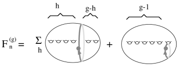
Figure 4: Topologically inequivalent ways to wind a Hamiltonian cycle around a surface of genus $g$.

Equation (19) can be understood as follows (See Fig.4). When one cuts the surface $\Sigma_{g}$ along a Hamiltonian cycle, one is left with a (possibly disconnected) surface with two circular boundaries. If the surface remains connected, the surface obtained should be $\Sigma_{g-1}$ with two holes (the second term in Fig 4). If it becomes disconnected, one has $\Sigma_{h}$ and $\Sigma_{g-h}$ which are to be glued together along the Hamiltonian cycle to form $\Sigma_{g}$ (the first term in Fig 4). This exhausts all the possibilities. There are precisely $[\tfrac{g}{2}+2]$ topologically inequivalent sectors. Note that the summands for $h=h_{0}$ and $h=g-h_{0}$ in the first term in (19) belong to an identical topological sector. Equation (19) can be used to calculate contributions from each topological sectors as well as the sum $F^{(g)}_{n}$ using (8) and (9).

At this point, I am naturally led to define the ‘all-genus’ generating function

$$F(p,t)=\sum_{g=0}^{\infty}t^{g}\sum_{n=0}^{\infty}p^{n}F_{n}^{(g)}.$$ (20)

Notably, this simplifies the expression a lot. I find that

$$F(p,\tfrac{1}{N^{2}})=\frac{1}{2}\sum_{n=0}^{\infty}p^{n}\sum_{k=0}^{n}\binom{n}{k}\left\langle\frac{1}{N}\mathrm{tr}M^{k}\frac{1}{N}\mathrm{tr}M^{n-k}\right\rangle,$$ (21)

where $N$ is the dimension of the matrix variable $M$. The correlation function in the right hand side includes both connected and disconnected parts. In fact, I can easily recover (19) by expanding (21) in $1/N$.

I further rewrite (21) to have a simple integral expression. I obtain

$$F(p,\tfrac{1}{N^{2}})= \frac{1}{2}\sum_{n=0}^{\infty}p^{n}\left(\frac{\partial}{\partial t_{1}}+\frac{\partial}{\partial t_{2}}\right)^{n}\left.\left\langle\frac{1}{N}\mathrm{tr}e^{t_{1}M}\frac{1}{N}\mathrm{tr}e^{t_{2}M}\right\rangle\right|_{t_{1},t_{2}=0}$$

$$= \frac{1}{2}\int^{\infty}_{0}ds\ e^{-s}e^{ps\left(\frac{\partial}{\partial t_{1}}+\frac{\partial}{\partial t_{2}}\right)}\left.\left\langle\frac{1}{N}\mathrm{tr}\ e^{t_{1}M}\frac{1}{N}\mathrm{tr}\ e^{t_{2}M}\right\rangle\right|_{t_{1},t_{2}=0}$$

$$= \frac{1}{2}\int^{\infty}_{0}ds\ e^{-s}\left\langle\left(\frac{1}{N}\mathrm{tr}\ e^{spM}\right)^{2}\right\rangle.$$ (22)

In the above derivation, I have made use of the integral expression of the $\Gamma$-function. It can be easily checked that the coefficients of $N^{-2}$ and $N^{0}$ in (22) exactly agree with eq. (3) and the result in ref.[6], respectively.

The expression (22) is not only simple but also practically useful. It enables one to calculate $F^{(g)}_{n}$ by the method of orthogonal polynomials [24, 25].

Because $F(p,\tfrac{1}{N^{2}})$ has been written as a correlation function of the gaussian hermitian matrix model in (22), the system should fall into the same universality class as the topological gravity or two-dimensional quantum gravity coupled to $c=-2$ matter [30, Subsection 9.3]. Namely, the double scaling behavior

$$F(p,\tfrac{1}{N^{2}})\sim(\tfrac{1}{4}-p)^{2}f(N^{2}(\tfrac{1}{4}-p)^{3})$$ (23)

or equivalently the large-$n$ asymptotics

$$F^{(g)}_{n}\sim 4^{n}n^{3g-3}\ \ \ (n\rightarrow\infty)$$ (24)

is implied.

The central charge $c=-2$ was previously obtained by Duplantier and Kostov in the analysis of the dense phase of polymers on random lattices of arbitrary genus [29]. They made use of the hermitian O($n$) multi-matrix model with a non-gaussian interaction, where $1/N$-expansion corresponds to the genus expansion and the $n\rightarrow 0$ guarantees that a Hamiltonian cycle is connected [5]. In the present analysis of the compact polymer, I have written the generating function $F(p,\tfrac{1}{N^{2}})$, whose $1/N$-expansion is again the genus expansion, in terms of the simplest matrix model: the hermitian gaussian 1-matrix model without any limiting procedure.

5 Discussions

I have obtained the generating function for the number of Hamiltonian cycles on surfaces of arbitrary genus. For genus $g=1$, the contributions from winding and non-winding sector are determined. This can be done for an arbitrary genus by eq. (19).

The limit of large graphs (24), is consistent with the assertion that the system is in the same universality class as the $c=-2$ quantum gravity [5, 6]. In the way of calculating the generating function, I have made use of microscopic loop amplitudes of the gaussian hermitian 1-matrix model.

Many deep connections have been found between the gaussian hermitian matrix model and the $c=-2$ quantum gravity since the first calculation of quantum gravity beyond the spherical limit at $c=-2$ by Kostov and Mehta [31]. They have written the free energy at genus $g$ in terms of correlation functions of the gaussian hermitian matrix model at order $1/N^{2g}$. In contrast, $F^{(g)}(p)$ in the present case gets contributions from correlators at all orders above $1/N^{2g}$. The free energy in ref. [31] is the generating function for the number of maximal trees on graphs, while $F^{(g)}(p)$ here generates the number of Hamiltonian cycles.

It is interesting to compare eq.(24) with the number of connected trivalent fat graphs with $n$ vertices in the absence of Hamiltonian cycles [5]. The latter behaves as [23, 32, 33].

$$\hat{F}_{n}^{(g)}:=\sum_{G\in S^{n,g}}1\times\frac{1}{\#\mathrm{Aut\ }G}\sim(2\cdot 3^{3/4})^{n}n^{\frac{5}{2}g-\frac{7}{2}}.$$ (25)

I introduce the ‘random average’ of $\mathcal{H}(G)$ among $G$’s in $S^{n,g}$ by

$$\langle\mathcal{H}(G)\rangle_{G\in S^{n,g}}:=\frac{F_{n}^{(g)}}{\hat{F}_{n}^{(g)}}\sim(2\cdot 3^{-3/4})^{n}n^{(g+1)/2}=(0.877383\cdots)^{n}n^{(g+1)/2}.$$ (26)

This behavior may be compared to the case of the fixed flat lattice with the same coordination number 3, i.e. the hexagonal lattice. The number $\mathcal{H}(G)$ for the hexagonal lattice grows as [14, 15]

$$\mathcal{H}(G)\sim(3^{3/4}/2)^{n}n^{\gamma}\sim(1.13975\cdots)^{n}n^{\gamma}\quad(n:=\#G),$$ (27)

where the conformational exponent $\gamma$ is believed to be unity. Having this behavior of fixed regular lattice in mind, it is puzzling that the average $\langle\mathcal{H}(G)\rangle_{G\in S^{n,g}}$ decreases as $n$ grows.

These totally different behaviors of (26) and (27) can be understood as follows. In the ensemble $S^{n,g}$ for arbitrarily large $n$, there are many $G$’s with $\mathcal{H}(G)=0$. In fact, if a graph admits a Hamiltonian cycle, then the graph should be $2$-edge-connected. Thus, as pointed out in ref. [5], $G$ does not admit any Hamiltonian cycles if $G$ is one-particle reducible. Therefore it is more natural to consider the random average over $\bar{S}^{n,g}$, the restriction of $S^{n,g}$ to one-particle irreducible graphs. It is known that the number of one-particle irreducible graphs grows as [23]

$$\bar{F}_{n}^{(g)}:=\sum_{G\in\bar{S}^{n,g}}1\times\frac{1}{\#\mathrm{Aut\ }G}\sim(2^{-1/2}\cdot 3^{3/2})^{n}n^{\frac{5}{2}g-\frac{7}{2}}.$$ (28)

Therefore I obtain

$$\!\!\!\!\!\langle\mathcal{H}(G)\rangle_{G\in\bar{S}^{n,g}}:=\frac{F_{n}^{(g)}}{\bar{F}_{n}^{(g)}}\sim(2^{5/2}\cdot 3^{-3/2})^{n}n^{(g+1)/2}=(1.08866\cdots)^{n}n^{(g+1)/2}.$$ (29)

It is interesting to note that the value $1.08866\cdots$ is near to the corresponding value $1.13975\cdots$ for the fixed hexagonal lattice as well as the field theoretic estimate $3/e=1.10364\cdots$ for regular lattices with coordination number three [34, 2]. For $g=1$, the power correction in (29) becomes $n^{1}$, which coincides with that of the fixed flat hexagonal lattice (27). One is tempted to speculate that Hamiltonian cycles on random lattices resembles those on a regular lattice with the identical coordination number and the identical average curvature (zero for $g=1$) once one restricts oneself to one-particle irreducible graphs.

In ref. [5], Eynard, Guitter and Kristjansen have mapped the problem of counting Hamiltonian cycles on planar random lattices to that of O($n$) model in the $n\rightarrow 0$ limit on the sphere. Their Hamiltonian cycles are not furnished with directions and base points. The $1/N$-expansion of their model should contain the information of the number of Hamiltonian cycles on surfaces of arbitrary genus. I believe that their approach and the present one are complementary each other.

Equation (22) formally resembles the expression for macroscopic loop amplitudes of the one-matrix model in ref. [35]. It may be interesting to translate the present analysis into the language of free fermions.

Acknowledgments

I thank Shinobu Hikami and Mitsuhiro Kato for useful discussions. This work was supported by the Ministry of Education, Science and Culture under Grant 08454106 and 10740108 and by Japan Science and Technology Corporation under CREST.

References

- [1] J. L. Jacobsen and J. Kondev, Field theory of compact polymers on the square lattice, Preprint cond-mat/9804048.
- [2] S. Higuchi, Phys. Rev. E58 (1998) 128, cond-mat/9711152.
- [3] J. Kondev and J. L. Jacobsen, Conformational entropy of compact polymers, Preprint cond-mat/9805178.
- [4] J. Kondev, J. de Gier, and B. Nienhuis, J. Phys. A 29 (1996) 6489.
- [5] B. Eynard, E. Guitter, and C. Kristjansen, Nucl. Phys. B528 (1998) 523.
- [6] S. Higuchi, Mod. Phys. Lett. A13 (1998) 727, cond-mat/9801307.
- [7] J. des Cloizeaux and G. Jannik, Polymers in solution: their modelling and structure, Clarendon Press, Oxford, 1987.
- [8] H. S. Chan and K. A. Dill, Macromolecules 22 (1989) 4559.
- [9] C. J. Camacho and D. Thirumalai, Phys. Rev. Lett. 71 (1993) 2505.
- [10] S. Doniach, T. Garel, and H. Orland, J. Chem. Phys. 105 (1996) 1601.
- [11] P. W. Kasteleyn, Physica(Utrecht) 29 (1963) 1329.
- [12] E. H. Lieb, Phys. Rev. Lett. 18 (1967) 692.
- [13] T. G. Schmalz, G. E. Hite, and D. J. Klein, J. Phys. A 17 (1984) 445.
- [14] J. Suzuki, J. Phys. Soc. Japan 57 (1988) 687.
- [15] M. Batchelor, J. Suzuki, and C. Yung, Phys. Rev. Lett. 73 (1994) 2646.
- [16] M. T. Batchelor, H. W. J. Blöte, B. Nienhuis, and C. M. Yung, J. Phys. A 29 (1996) L399.
- [17] V. G. Knizhnik, A. M. Polyakov, and A. B. Zamolodchikov, Mod. Phys. Lett. A3 (1988) 819.
- [18] J. Distler and H. Kawai, Nucl. Phys. B321 (1989) 509.
- [19] F. David, Mod. Phys. Lett. A3 (1988) 1651.
- [20] H. W. J. Blöte and B. Nienhuis, Phys. Rev. Lett. 72 (1994) 1372.
- [21] B. Duplantier and H. Saleur, Nucl. Phys. B290[FS20] (1987) 291.
- [22] G. ’t Hooft, Nucl. Phys. B72 (1974) 461.
- [23] E. Brézin, C. Itzykson, G. Parisi, and J.-B. Zuber, Comm. Math. Phys. 59 (1978) 35.
- [24] D. Bessis, C. Itzykson, and J.-B. Zuber, Adv. in Appl. Math. 109 (1980) 1.
- [25] M. L. Mehta, Random Matrices, Academic Press, revised and enlarged second edition, 1991.
- [26] V. A. Kazakov, Mod. Phys. Lett. A4 (1989) 2125.
- [27] J. Ambjørn, L. Chekhov, C. F. Kristjansen, and Y. Makeenko, Nucl. Phys. B404 (1993) 127, erratum ibid. B449(1995)681.
- [28] B. Duplantier and I. K. Kostov, Phys. Rev. Lett. 61 (1988) 1433.
- [29] B. Duplantier and I. K. Kostov, Nucl. Phys. B340 (1990) 491.
- [30] P. Ginsparg and G. Moore, Lectures on gravity and string theory, hep-th/9304011.
- [31] I. K. Kostov and M. L. Mehta, Phys. Lett. B189 (1987) 118.
- [32] V. A. Kazakov, I. K. Kostov, and A. A. Migdal, Phys. Lett. 157B (1985) 295.
- [33] F. David, Nucl. Phys. B257[FS14] (1985) 45.
- [34] H. Orland, C. Itzykson, and C. de Dominicis, J. Physique 46 (1985) L353.
- [35] T. Banks, M. E. Douglas, N. Seiberg, and S. H. Shenker, Phys. Lett. B238 (1990) 279.