Superconductivity of Quasi-One and Quasi-Two Dimensional Tight-Binding Electrons in Magnetic Field

In the semiclassical approximation, the upper critical field $H_{c2}(T)$ of isotropic superconductors is derived from Ginzburg-Landau-Abrikosov-Gor’kov (GLAG) theory. ${}^{\hbox{\immediate{\bf{?}},\penalty 1000\hskip 0.91003pt plus 0.70004pt minus 0.70004pt{\bf{?}})}}$ Lawrence and Doniach ${}^{\hbox{\immediate{\bf{?}})}}$ have applied GLAG theory to layered superconductors. Klemm et al. ${}^{\hbox{\immediate{\bf{?}})}}$ and Bulaevskii and Guseinov. ${}^{\hbox{\immediate{\bf{?}})}}$ have shown that $H_{c2}(T)$ displays upward curvature when the magnetic field is applied parallel to the layer. When the coherence length $\xi(T)$ of the order parameter becomes smaller than the distance of layers, $H_{c2}(T)$ is infinite. However, these results are based on a semiclassical approximation, in which only the phase of the wave function of electrons is changed by magnetic field.

It was shown that the quantum effect of the electrons in the BCS theory lead to reentrant behavior in high magnetic field.  ${}^{\hbox{\immediate{\bf{?}},\penalty 1000\hskip 0.91003pt plus 0.70004pt minus 0.70004pt{\bf{?}},\penalty 1000\hskip 0.91003pt plus 0.70004pt minus 0.70004pt{\bf{?}},\penalty 1000\hskip 0.91003pt plus 0.70004pt minus 0.70004pt{\bf{?}},\penalty 1000\hskip 0.91003pt plus 0.70004pt minus 0.70004pt{\bf{?}},\penalty 1000\hskip 0.91003pt plus 0.70004pt minus 0.70004pt{\bf{?}})}}$ The reentrance of the superconductivity due to Landau quantization has attracted theoretical interest. ${}^{\hbox{\immediate{?},\penalty 1000\hskip 0.91003pt plus 0.70004pt minus 0.70004pt{?})}}$ In that case, Cooper pairs are formed between electrons at the lowest Landau level in strong magnetic field. However, when only the lowest Landau level is filled in the three dimensional case, the system can be treated as a 1D system, i.e., energy depends only on the momentum parallel to the magnetic field, and it has been shown that the system is unstable to the density wave state rather than the superconductivity. ${}^{\hbox{\immediate{\bf{?}},\penalty 1000\hskip 0.91003pt plus 0.70004pt minus 0.70004pt{\bf{?}})}}$

Recently, superconductivity in strong magnetic field is observed in organic superconductors (TMTSF)$\mbox{}_{2}$PF$\mbox{}_{6}$.  ${}^{\hbox{\immediate{\bf{?}},\penalty 1000\hskip 0.91003pt plus 0.70004pt minus 0.70004pt{\bf{?}})}}$ Similar result has also been observed in (TMTSF)$\mbox{}_{2}$ClO$\mbox{}_{4}$. ${}^{\hbox{\immediate{?},\penalty 1000\hskip 0.91003pt plus 0.70004pt minus 0.70004pt{\bf{?}})}}$ Organic superconductors (TMTSF)$\mbox{}_{2}$X are well described by quarter-filled tight-binding electrons (actually holes) with $t_{a}\sim 3000$K, $t_{b}/t_{a}\sim 0.1$, $t_{c}/t_{a}\sim 0.003$. Since the magnetic field of 10T corresponds to $\phi/\phi_{0}\sim 1/1000$ in (TMTSF)$\mbox{}_{2}$X, where $\phi$ is flux per unit area and $\phi_{0}$ is the flux quantum, the effect of the Landau level quantization is negligible. However, when the magnetic field is applied perpendicular to plane, field-induced spin density wave (FISDW) is stabilized. The existence of FISDW shows that the quantum effect is important in quasi-one dimensional (Q1D) systems and the semiclassical approximation of the magnetic field is not appropriate in these systems.

Lebed ${}^{\hbox{\immediate{?})}}$ has predicted that the Q1D superconductors should exhibit superconductivity in a strong magnetic field. The superconductivity observed in (TMTSF)$\mbox{}_{2}$PF$\mbox{}_{6}$ and (TMTSF)$\mbox{}_{2}$ClO$\mbox{}_{4}$ is thought to be the realization of the Q1D superconductivity in strong magnetic field. The mechanism of the reentrance of Q1D superconductivity is similar to that of FISDW. In the presence of the magnetic field, the dimensionality of the system is reduced. When the magnetic field is applied in the $c$ direction in the system with hopping matrix elements $t_{a}\gg t_{b}\gg t_{c}$, the effect of $t_{b}$, which makes the nesting of the Fermi surface imperfect with the imperfectness parameter of the order of $t_{b}^{2}/t_{a}$, disappears and spin-density-wave is induced. When the magnetic field is applied in $b$ direction, the nesting of the Fermi surface stays imperfect but the orbital frustration is removed if we take account of the eigenstates in the magnetic field. In the Q1D case, the magnetic field necessary for the reentrance of the superconductivity is much smaller than that in the case of Landau level quantization. Dupuis et al. ${}^{\hbox{\immediate{?})}}$ have extensively studied the mean-field transition line $T_{c}(H)$ of Q1D superconductors and shown the cascade transitions to the superconducting states. We have studied the anisotropic superconductivity with line nodes of the energy gap,  ${}^{\hbox{\immediate{?})}}$ which is thought to be realized in organic superconductors (TMTSF)$\mbox{}_{2}$X. In these papers, ${}^{\hbox{\immediate{?},\penalty 1000\hskip 0.91003pt plus 0.70004pt minus 0.70004pt{?},\penalty 1000\hskip 0.91003pt plus 0.70004pt minus 0.70004pt{?})}}$ however, only warping of the Fermi surface in $k_{z}$ direction normal to $H$ has been considered, and that in $k_{y}$ direction is neglected.

As $t_{b}$ increases, quasi-one dimensional system turns into quasi-two dimensional system. Quasi-two-dimensional (Q2D) electrons, for example, $\beta$-(BEDT-TTF)$\mbox{}_{2}$I$\mbox{}_{3}$ ($t_{a}\sim 3000$K, $t_{b}/t_{a}\sim 0.5$ and $t_{c}/t_{a}\sim 0.02$) have a two-dimensional cylindrical Fermi surface with a weak warping along $k_{z}$ direction. When the magnetic field $H$ is applied in $b$ direction, the electrons move either in open orbit reaching the zone boundary or in closed orbit as is schematically shown in Fig.1.

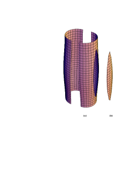
Fig.  1: Fermi surface of a quasi-two dimensional conductor is drawn. In the presence of magnetic field along $k_{y}$, the electrons move open orbit (a) and closed orbit (b).

The former gives the similar effect as in Q1D superconductors. It have been discussed by Lebed ${}^{\hbox{\immediate{?})}}$ and Dupuis et al.  ${}^{\hbox{\immediate{?})}}$ that the Q2D superconductors will evolve from the GLAG region to reentrant phase. Recently, Lebed and Yamaji ${}^{\hbox{\immediate{?})}}$ have calculated the mean field transition temperature of Q2D superconductor and shown the reentrant behavior. They have used the parabolic band in the conducting plane, i.e. the lattice structure is neglected in the plane.

In this paper, we calculate the mean field transition temperature numerically by taking account of the eigenstates of three-dimensional tight-binding electrons in magnetic field. In this formation, we can treat both Q1D and Q2D systems by changing $t_{b}/t_{a}$.

We start from the tight-binding Hamiltonian (we take $\hbar=k_{\rm B}=c_{0}=1$, where $c_{0}$ is a light velocity, throughout the paper),

$${\cal H}_{0} = -t_{a}\sum_{(i,j)_{a},\sigma}e^{{\rm i}\theta_{ij}}c^{{\dagger}}_{i,\sigma}c_{j,\sigma}-t_{b}\sum_{(i,j)_{b},\sigma}e^{{\rm i}\theta_{ij}}c^{{\dagger}}_{i,\sigma}c_{j,\sigma}$$ (1)

$$-t_{c}\sum_{(i,j)_{c},\sigma}e^{{\rm i}\theta_{ij}}c^{{\dagger}}_{i,\sigma}c_{j,\sigma}-\mu\sum_{i,\sigma}c^{{\dagger}}_{i,\sigma}c_{i,\sigma}$$

$$-\sum_{i,\sigma}\sigma\mu_{\rm B}Hc^{{\dagger}}_{i,\sigma}c_{i,\sigma},$$

where $c^{{\dagger}}_{i,\sigma}$ and $c_{i,\sigma}$ are creation and annihilation operators, $\mu$ is chemical potential and $\sigma\mu_{\rm B}H$ is the Zeeman energy for $\uparrow$ ($\downarrow$) spin ($\sigma=+(-)$) and

$$\theta_{ij}=\frac{2\pi}{\phi_{0}}\int^{j}_{i}\mbox{\boldmath$A$}d\mbox{\boldmath$l$}.$$ (2)

In the above $A$ is the vector potential. We consider the anisotropic system with the hopping matrix elements $t_{a}\geq t_{b}\gg t_{c}$. We neglect the field dependence of $\mu$, since the energy gap due to the magnetic field is very small in the anisotropic system with $\phi/\phi_{0}\ll 1$ except for the bottom and the top of the band.

In this paper the magnetic field $H$ is applied in the $b$ direction. We take the vector potential $A$ as ${\mbox{\boldmath$A$}}=(0,0,-Hx)$ and the non-interacting Hamiltonian is written as

$${\cal H}_{0}=$$

$$\sum_{\sigma,\mbox{{\mbox{\boldmath$k$}}}}C^{{\dagger}}_{\sigma}\left(\begin{array}[]{ccc}\ddots&&V^{*}\\ &\begin{array}[]{ccc}M_{-1}&V&0\\ V^{*}&M_{0}&V\\ 0&V^{*}&M_{1}\end{array}&\\ V&&\ddots\end{array}\right)C_{\sigma},$$ (9)

where

$$M_{n}=-2t_{a}\cos[a(k_{x}+nG)]-2t_{b}\cos(bk_{y})-\mu-\sigma\mu_{\rm B}H,$$ (10)

$$V=-t_{c}e^{{\rm i}ck_{z}},$$ (11)

$$C^{{\dagger}}_{\sigma}=(\cdots,c^{{\dagger}}_{\sigma}({\mbox{\boldmath$k$}}-{\mbox{\boldmath$G$}}),c^{{\dagger}}_{\sigma}({\mbox{\boldmath$k$}}),c^{{\dagger}}_{\sigma}({\mbox{\boldmath$k$}}+{\mbox{\boldmath$G$}}),\cdots),$$ (12)

$${\mbox{\boldmath$G$}}=(G,0,0)=\left(\frac{2\pi}{a}\frac{\phi}{\phi_{0}},0,0\right).$$ (13)

The creation operators of electrons can be written in terms of the creation operators of the eigenstates ($\Psi^{{\dagger}}_{\sigma}(n,{\mbox{\boldmath$k$}})$) of eq.(3) as

$$c^{{\dagger}}_{\sigma}({\mbox{\boldmath$k$}}+m{\mbox{\boldmath$G$}})=e^{{\rm i}mck_{z}}\sum_{n}\phi^{*}_{k_{x},k_{z}}(m,n)\Psi^{{\dagger}}_{\sigma}(n,{\mbox{\boldmath$k$}}),$$ (14)

where $m$ and $n$ are integers.

Using eq.(8), the real space one-particle Green’s function is given by

$$G_{\sigma}({\mbox{\boldmath$r$}},{\mbox{\boldmath$r$}}^{\prime},{\rm i}\omega_{l}) = -\int^{\beta}_{0}d\tau e^{{\rm i}\omega_{l}\tau}\left<T_{\tau}C_{{\mbox{\boldmath$r$}},\sigma}(\tau)C^{{\dagger}}_{{\mbox{\boldmath$r$}}^{\prime},\sigma}(0)\right>$$ (15)

$$= \sum_{{\mbox{\boldmath$k$}},n}\sum_{m,m^{\prime}}\frac{\phi_{k_{x},k_{z}}(m,n)\phi^{*}_{k_{x},k_{z}}(m^{\prime},n)}{{\rm i}\omega_{l}-\varepsilon_{n,{\mbox{\boldmath$k$}},\sigma}}$$

$$\times e^{{\rm i}(m^{\prime}-m)ck_{z}}e^{{\rm i}({\mbox{\boldmath$r$}}^{\prime}-{\mbox{\boldmath$r$}})\cdot{\mbox{\boldmath$k$}}+{\rm i}(m^{\prime}{\mbox{\boldmath$r$}}^{\prime}-m{\mbox{\boldmath$r$}})\cdot{\mbox{\boldmath$G$}}},$$

where $\omega_{l}=(2l+1)\pi T$ is a Matsubara frequency and $l$ is integer. In this paper, we neglect the Zeeman energy for simplicity. The coefficients $\phi_{k_{x},k_{z}}(m,n)$ and eigenvalues

$$\varepsilon_{n,{\mbox{\boldmath$k$}}}=\epsilon(n,k_{x},k_{z})-2t_{b}\cos(bk_{y})-\mu,$$ (16)

can be calculated by diagonalizing the matrix in eq.(3) numerically, where $\epsilon(n,k_{x},k_{z})$ is the eigenvalue of eq.(3) for $-2t_{b}\cos(bk_{y})-\mu=0$. If $\phi/\phi_{0}=p/q$, where $p$ and $q$ are mutually prime integers, the matrix size of eq.(3) is $q\times q$ and the magnetic Brillouin zone is given by $-\pi/(qa)<k_{x}<\pi/(qa)$.

Since we are interested in the instability to the superconductivity in the quarter-filled tight-binding electrons at the temperature much smaller than the band width, the eigenstates near the top of the band are not important in the anisotropic hopping case ($t_{c}\ll t_{a}$). Thus, we calculate only $3/4\sim 1/2$ of the states from the bottom of the band in eq.(3) by neglecting $V$ and $V^{*}$ for $c(\mbox{\boldmath$k$}+n\mbox{\boldmath$G$})$ with $|k_{x}+nG|\geq(3/4)\pi/a$ or $|k_{x}+nG|\geq(1/2)\pi/a$. We have checked that the result is not changed by this approximation. In this approximation, we can take the matrix size as $\sim[\pi/G]\times[\pi/G]$ and $-G/2<k_{x}<G/2$. The eigenvalues and coefficients do not depend on $k_{z}$ in this approximation and we write $\epsilon(n,k_{x},k_{z})=\epsilon(n,k_{x})$ and $\phi_{k_{x},k_{z}}(m,n)=\phi_{k_{x}}(m,n)$ ($\phi_{k_{x}}(m,n)$ can be taken real).

In the mean field approximation, the linearized gap equation for s-wave pairing in coordinate representation is obtained as

$$\Delta({\mbox{\boldmath$r$}})=\lambda\int d{\mbox{\boldmath$r$}}^{\prime}K({\mbox{\boldmath$r$}},{\mbox{\boldmath$r$}}^{\prime})\Delta({\mbox{\boldmath$r$}}^{\prime}),$$ (17)

where

$$K({\mbox{\boldmath$r$}},{\mbox{\boldmath$r$}}^{\prime})\equiv T\sum_{\omega_{l}}G({\mbox{\boldmath$r$}},{\mbox{\boldmath$r$}}^{\prime},{\rm i}\omega_{l})G({\mbox{\boldmath$r$}},{\mbox{\boldmath$r$}}^{\prime},-{\rm i}\omega_{l}),$$ (18)

and $\lambda$ is the coupling constant. We write

$$\Delta(x)=\sum_{q_{x},N}e^{{\rm i}(q_{x}+NG)x}\Delta_{N}(q_{x}),$$ (19)

where $q_{x}$ is taken as $-G/2<q_{x}\leq G/2$. For even $N$, using eqs.(9) and (13), linearized gap equation is written as a matrix equation

$$\Delta_{2j}(q_{x})=\lambda\sum_{j^{\prime}}\Pi_{2j,2j^{\prime}}\Delta_{2j^{\prime}}(q_{x}),$$ (20)

where

$$\Pi_{2j,2j^{\prime}}(q_{x})=\sum_{k_{x},k_{y}}\sum_{n,n^{\prime}}\sum_{m}\phi_{k_{x}}(m-j,n)\phi_{k_{x}}(m-j^{\prime},n)$$

$$\times\phi_{-k_{x}}(-m-j,n^{\prime})\phi_{-k_{x}}(-m-j^{\prime},n^{\prime})$$

$$\times\frac{1-f(\varepsilon_{n,k_{x},k_{y}})-f(\varepsilon_{n^{\prime},-k_{x}-q_{x},-k_{y}})}{2(\varepsilon_{n,k_{x},k_{y}}+\varepsilon_{n^{\prime},-k_{x}-q_{x},-k_{y}})},$$ (21)

where $f(\varepsilon)$ is the Fermi distribution function.

For odd $N$, we get

$$\Delta_{2j+1}(q_{x})=\lambda\sum_{j^{\prime}}\Pi_{2j+1,2j^{\prime}+1}\Delta_{2j^{\prime}+1}(q_{x}),$$ (22)

where

$$\Pi_{2j+1,2j^{\prime}+1}(q_{x})=\sum_{k_{x},k_{y}}\sum_{n,n^{\prime}}\sum_{m}\phi_{k_{x}}(m-j,n)\phi_{k_{x}}(m-j^{\prime},n)$$

$$\times\phi_{-k_{x}}(-m-j-1,n^{\prime})\phi_{-k_{x}}(-m-j^{\prime}-1,n^{\prime})$$

$$\times\frac{1-f(\varepsilon_{n,k_{x},k_{y}})-f(\varepsilon_{n^{\prime},-k_{x}-q_{x},-k_{y}})}{2(\varepsilon_{n,k_{x},k_{y}}+\varepsilon_{n^{\prime},-k_{x}-q_{x},-k_{y}})}.$$ (23)

The transition line is given by $1-g\lambda=0$ for eq.(14) and eq.(16), where $g$ is the maximum eigenvalue of the matrix $\Pi$ of the even part or the odd part. In this paper, we calculate the field dependence of the effective coupling constant $g$ at low temperature instead of calculating the transition temperature. In the BCS theory Cooper pairs are formed by electrons with wave numbers $k$ and $-\mbox{\boldmath$k$}$ and the energy of these states are different in the presence of magnetic field, which causes the orbital frustration. In the formulation of eqs.(14) and (16), however, we can take the states ($n,\mbox{\boldmath$k$}$) and ($n^{\prime},-\mbox{\boldmath$k$}$) which have the same energy $\varepsilon_{n,k_{x},k_{y}}=\varepsilon_{n^{\prime},-k_{x},-k_{y}}$. Therefore the superconductivity is not destroyed by the orbital frustration in the strong magnetic field. This is the similar mechanism for the FISDW. ${}^{\hbox{\immediate{\bf{?}})}}$ In the weak magnetic field the coefficient $\phi_{k_{x}}(m,n)$ becomes small and the present results reproduce the GLAG results.

For the Q1D superconductors with open Fermi surface, the energy dispersion in $k_{x}$ is taken to be linear and the Fermi velocity and the density of states are taken to be constant in the previous calculations. ${}^{\hbox{\immediate{?},\penalty 1000\hskip 0.91003pt plus 0.70004pt minus 0.70004pt{?},\penalty 1000\hskip 0.91003pt plus 0.70004pt minus 0.70004pt{?})}}$ As a first approximation, we take

$$M_{n}\approx{\rm sgn}(n)v_{\rm F}(k_{y})(|k_{x}+nG|-k_{\rm F}),$$ (24)

where $v_{F}(k_{y})=2t_{a}a\sin ak_{\rm F}(k_{y})$ and $k_{F}(k_{y})$ are the Fermi velocity and Fermi wave number depending on $k_{y}$, respectively. We may diagonalize the matrix for $k_{x}+nG\sim k_{\rm F}(k_{y})$ and $k_{x}+nG\sim-k_{\rm F}(k_{y})$ independently, as in the previous calculations. Then the eigenstates are given with the coefficients,

$$\phi_{k_{x}}(m,n)\cong J_{m-n}\left(\frac{2t_{c}}{v_{\rm F}(k_{y})G}\right)\ \ {\rm for}\ n,m>0$$ (25)

and

$$\phi_{k_{x}}(m,n)\cong J_{-m+n}\left(\frac{2t_{c}}{v_{\rm F}(k_{y})G}\right)\ \ {\rm for}\ n,m<0,$$ (26)

where $J$ is the Bessel function. Note that in this approximation $\phi_{k_{x}}(m,n)$ does not depend on $k_{x}$ but it depends on $k_{y}$ through $v_{\rm F}(k_{y})$. In Fig.2, we plot the effective coupling constant $g/g_{0}$ obtained by this linearized dispersion by solid, dashed, and dot-dashed lines as a function of $aG/(2\pi)$, where $g_{0}$ is the effective coupling constant for $t_{c}=0$ , which corresponds to that in the absence of magnetic field.

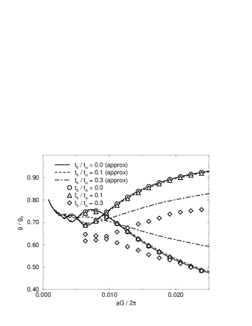
Fig.  2: Effective coupling constant as a function of $aG/(2\pi)$ in the case of $t_{c}/t_{a}=0.02$ and $T/t_{a}=0.001$. In strong magnetic field, the effective coupling constant obtained by diagonalizing the even part of the matrix $\Pi$ reaches to that of zero magnetic field. The coupling constant for odd part gives zero in strong magnetic field. Solid, dashed and dot-dashed lines are obtained in the approximation of linearized energy dispersion. Circle, triangle and diamond symbols are obtained without that approximation.

In strong magnetic field, the effective coupling constant of the even part is increased and that of the odd part is decreased for each $t_{b}/t_{a}$. In the case of $t_{b}=0$, we get the previous result. ${}^{\hbox{\immediate{?})}}$ As can be seen in Fig.2, for larger $t_{b}/t_{a}$ the oscillation becomes small.

Next, we calculate the effective coupling constant $g/g_{0}$ by numerically diagonalizing the lower $3/4$ or $1/2$ of the matrix in eq.(3) without using the approximation eq.(18) and we plot the results as circles, triangles and diamonds in Fig.2. For $t_{b}/t_{a}=0.1$ the results are almost same as that obtained by the approximation with the $k_{y}$-dependent Fermi velocity (eq.(18)) as expected, but the deviation is large for larger $t_{b}/t_{a}$.

We also study the quasi-two dimensional superconductor with $t_{b}/t_{a}=0.5$ and $1.0$. In Fig.3 we plot the effective coupling constant as a function of $aG/(2\pi)$. As is seen in Fig.3, the effective coupling constant reaches to that for $t_{c}=0$ as magnetic field is increased.

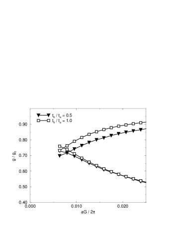
Fig.  3: Effective coupling constant as a function of $aG/(2\pi)$ in the case of $t_{c}/t_{a}=0.02$ and $T/t_{a}=0.001$.

The reason why $g/g_{0}$ is small for $t_{b}/t_{a}=0.3$ is as follows. In Fig.4, we plot the effective coupling constant as a function of $t_{b}/t_{a}$. In the case of $t_{c}=0$, there is a logarithmic divergence at about $t_{b}/t_{a}\sim 0.3$, which is van Hove singularity for the quarter-filled band.

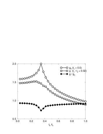
Fig.  4: Effective coupling constant as a function of $t_{b}/t_{a}$ at $aG/(2\pi)$=0.025 and $T/t_{a}=0.001$.

Therefore, the effective coupling constant normalizes by that for $t_{c}=0$ is small for $t_{b}/t_{a}\sim 0.3$.

In this paper we have neglected the Zeeman term for simplicity. However, we can calculate the transition line with Zeeman term in this expression. The Zeeman term does not play any important role for the equal-spin-pairing case of the spin triplet. If the Zeeman energy is taken into account, the transition temperature of spin singlet is reduced due to the effect of Pauli pair-breaking except for the Q1D case ($t_{b}=0$). The superconductivity of Q1D systems is not completely destroyed, ${}^{\hbox{\immediate{?},\penalty 1000\hskip 0.91003pt plus 0.70004pt minus 0.70004pt{?},\penalty 1000\hskip 0.91003pt plus 0.70004pt minus 0.70004pt{?})}}$ since half of the density of states is available to make Cooper pairs for the Larkin-Ovchinnikov-Fulde-Ferrell (LOFF) state, ${}^{\hbox{\immediate{\bf{?}},\penalty 1000\hskip 0.91003pt plus 0.70004pt minus 0.70004pt{\bf{?}})}}$ as in the pure 1D case. ${}^{\hbox{\immediate{\bf{?}},\penalty 1000\hskip 0.91003pt plus 0.70004pt minus 0.70004pt{\bf{?}},\penalty 1000\hskip 0.91003pt plus 0.70004pt minus 0.70004pt{\bf{?}})}}$

In conclusion, we have shown the transition lines of quasi-one dimensional and quasi-two dimensional superconductors in tight-binding model. The Green function in Q1D systems is described by the Bessel function if we apply the approximation that the energy dispersion in $k_{x}$ direction is taken to be linear. In this paper, we have shown that the Green function of the tight-binding electrons is numerically calculated without using the linearization of the energy dispersion. In the strong magnetic field Cooper pairs are formed in the eigenstates with the same energy. We have obtained the transition line $T_{c}(H)$ for both Q1D and Q2D cases. As $H$ becomes large, $T_{c}(H)$ increases oscillationally in both cases.

References

References

[1] A. A. Abrikosov: Zh. Eksp Teor. Fiz. 32 (1957) 1442.
[2] L. P. Gor’kov: Zh. Eksp. Teor. Fiz. 37 (1959) 833.
[3] W. E. Lawrence and S. Doniach, in Proc. 12th Int. Conf.
Low Temp. Phys. Kyoto, edited by E. Kanda (Academic Press of Japan,
Kyoto, 1971),
p.361.
[4] R. A. Klemm, M. R. Beasley and A. Luther: J. Low Temp.
Phys.16, (1974) 607; R. A. Klemm, A. Luther and M. R. Beasley:
Phys. Rev. B 12 (1975) 877.
[5] L. N. Bulaevskii and A. A. Guseinov:
JETP Lett. 19 (1974) 382.
[6] A. G. Lebed: Pis’ma Zh. Eksp. Teor. Fiz. 44 (1986)
89; translation: JETP Lett. 44 (1986) 114.
[7] M. Rasolt and Z. Tešanović: Rev. Mod. Phys.
64 (1992) 709.
[8] H. Akera, A. H. MacDonald, S. M. Girvin and M. R.
Norman: Phys. Rev. Lett. 67 (1991) 2375.
[9] N. Dupuis, G. Montambaux and C. A. R S
de Melo: Phys. Rev. Lett. 70 (1993) 2613; N. Dupuis and G.
Montambaux:
Phys. Rev. B 49 (1994) 8993; N. Dupuis: Phys. Rev. B 51
(1995) 9074.
[10] Y. Hasegawa and M. Miyazaki: J. Phys. Soc. Jpn. 65
(1996) 1028; M. Miyazaki and Y. Hasegawa: J. Phys. Soc. Jpn. 65
(1996) 3238.
[11] A. G. Lebed and K. Yamaji: Phys. Rev. Lett. 70
(1998) 2697.
[12] S. A. Brazovskii: Sov. Phys. JETP 34 (1972) 1286,
35 (1972) 433.
[13] V. M. Yakovenko: Phys. Rev. B 47 (1993) 8851.
[14] I. J. Lee, M. J. Naughton, G. M. Danner and P. M.
Chaikin: Phys. Rev. Lett. 78, (1997) 3555.
[15] M. J. Naughton, I. J. Lee, P. M. Chaikin and G. M. Danner:
Synth. Met. 85 (1997) 1481.
[16] I. J. Lee, A. P. Hope, M. J. Leone and M. J. Naughton:
Appl. Supercond. 2 (1994) 753; Synth. Met. 70 (1995) 747.
[17] Y. Hasegawa, J. Phys. Soc. Jpn. 64 (1995) 2541.
[18] P. Fulde and A. Ferrell: Phys. Rev. 135 (1964)
A550.
[19] A. I. Larkin and Yu. N. Ovchinnikov: Sov. Phys. JETP
20 (1965) 762.
[20] A. I. Buzdin and V. V. Tugusev: Sov. Phys. JETP 58
(1983) 428.
[21] Y. Suzumura and K. Ishino: Prog. Theor. Phys. 70
(1983) 654.
[22] K. Machida and H. Nakanishi: Phys. Rev. B 30
(1984) 122.