Physical Model of Nernst Element

Abstract

Generation of electric power by the Nernst effect is a new application of a semiconductor. A key point of this proposal is to find materials with a high thermomagnetic figure-of-merit, which are called Nernst elements. In order to find candidates of the Nernst element, a physical model to describe its transport phenomena is needed. As the first model, we began with a parabolic two-band model in classical statistics. According to this model, we selected InSb as candidates of the Nernst element and measured their transport coefficients in magnetic fields up to 4 Tesla within a temperature region from 270K to 330K. In this region, we calculated transport coefficients numerically by our physical model. For InSb, experimental data are coincident with theoretical values in strong magnetic field.

1 Introduction

One of the authors, S. Y., proposed [1] the direct electric energy conversion of the heat from plasma by the Nernst effect in a fusion reactor, where a strong magnetic field is used to confine a high temperature fusion plasma. He called [1, 2] the element which induces the electric field in the presence of temperature gradient and magnetic field, as Nernst element. In his papers [1, 2], he also estimated the figure of merit of the Nernst element in a semiconductor model. In his results [1, 2], the Nernst element has high performance in low temperature region, that is, 300 – 500 K. Before his works, the Nernst element was studied in the 1960’s [3]. In those days, induction of the magnetic field had a lot of loss of energy. This is the reason why the Nernst element cannot be used. Nowadays an improvement on superconducting magnet gives us higher efficiency of the induction of the strong magnetic field. We started a measuring system of transport coefficients in the strong magnetic field to estimate efficiency of the Nernst element on a few years ago [4]. We need criteria to find materials with high efficiency. The first model is one-band model which was proposed by S. Y. However is model cannot explain the temperature dependence of the Nernst coefficient above the room temperature for intrinsic indium antimonide, InSb_X [4, 5]. We improved the one-band model to the two-band model. In this paper, we measured InSb_B which is doped Te heavier than InSb_X. Near room temperature, the sample InSb_B transits from the extrinsic region to the intrinsic region. To calculate transport coefficients of InSb_B in a magnetic field, we use the two-band model, In this paper, we report the calculations by the two-band model. (In Ref.  [6], we also measured and calculated transport coefficients of Ge in a magnetic field near room temperature.)

2 Theoretical calculations

As the physical model to describe transport phenomena of the material in the Nernst element, we use a parabolic two-band model in the classical statics. We have the following parameters of this model;

• $m_{\rm n}$ ($m_{\rm p}$): effective mass of electron (hole),

• $\varepsilon_{\rm D}$ ($\varepsilon_{\rm A}$) : energy level of a donor (an acceptor),

• $N_{\rm D}$ ($N_{\rm A}$) : concentration of donors (acceptors),

• $\mu_{\rm n}$ ($\mu_{\rm p}$) : mobility of an electron (a hole),

• $\varepsilon_{\rm G}$: energy gap, $\varepsilon_{\rm F}$: fermi energy.

Using these parameters, we obtain concentrations of carriers as follows:

$$n(T) = N_{\rm C}(T)\exp\left(\frac{\varepsilon_{\rm F}-\varepsilon_{\rm G}}{kT}\right),$$ (1)

$$p(T) = N_{\rm V}(T)\exp\left(\frac{-\varepsilon_{\rm F}}{kT}\right),$$ (2)

where $n(p)$ is the concentration of free electron (hole). Here $N_{\rm C}$ ($N_{\rm V}$), the effective density of state in the conduction (valence) band is given by

$$N_{\rm C}(T) = 2\left(\frac{2m_{\rm n}\pi kT}{h^{2}}\right)^{\frac{3}{2}},$$ (3)

$$N_{\rm V}(T) = 2\left(\frac{2m_{\rm p}\pi kT}{h^{2}}\right)^{\frac{3}{2}}.$$ (4)

We also obtain the concentration of electrons (holes) in the donor (acceptor) level, $n_{\rm D}$ ($p_{\rm A}$) as follows:

$$n_{\rm D} = N_{\rm D}\frac{1}{1+\frac{1}{2}\exp\left(-\frac{\varepsilon_{\rm D}-\varepsilon_{\rm G}+\varepsilon{\rm F}}{kT}\right)},$$ (5)

$$p_{\rm A} = N_{\rm A}\frac{1}{1+2\exp\left(-\frac{\varepsilon_{\rm A}-\varepsilon_{\rm F}}{kT}\right)}.$$ (6)

We suppose the charge neutrality as

$$N_{\rm D}-n_{\rm D}+p(T)=N_{\rm A}-p_{\rm A}(T)+n(T).$$ (7)

Substituting the concentrations of carriers with eqs. (1)-(6) in eq. (7), we obtain the following algebraic equation in value $x\equiv\exp\left(\varepsilon_{\rm F}/kT\right)$ as

$$sux^{4}+\left(u+N_{\rm A}s+stu\right)x^{3}+\left(N_{\rm A}-N_{\rm D}+ut-N_{\rm V}s\right)x^{2}$$

$$-\left(N_{\rm D}t+N_{\rm V}+N_{\rm D}st\right)x-N_{\rm V}t=0,$$ (8)

where

$$s = 2\exp\left(\frac{\varepsilon_{\rm D}-\varepsilon_{\rm G}}{kT}\right),$$

$$t = \frac{1}{2}\exp\left(\frac{\varepsilon_{\rm A}}{kT}\right),$$

$$u = N_{\rm C}\exp\left(-\frac{\varepsilon_{\rm G}}{kT}\right).$$ (9)

Using the fermi energy which is given from eqs. (8) and (9) , we can solve the Boltzmann equation of this model in a magnetic field with a perturbation theory and the relaxation time approximation. See Ref. [1] for details. Here we define the following parameters to simplify formulation as

$$\eta\equiv\frac{\varepsilon_{\rm A}}{kT},\gamma=\frac{2m_{\rm n}kT}{\hbar^{2}},\beta_{0}=\frac{\sqrt{\pi}\mu_{\rm n}B}{4z},\beta=\frac{\beta_{0}}{4}\gamma^{\frac{5}{2}}.$$ (10)

We also define the following integrals as

$$I_{i}\left(\beta_{0}\right) = 4\gamma^{-1}\int_{0}^{\infty}\frac{x^{i}\exp\left(\eta-x\right)}{1+\frac{\beta_{0}^{2}}{x}},$$ (11)

$$J_{j}\left(\beta_{0}\right) = 16\gamma^{-\frac{7}{2}}\int_{0}^{\infty}\frac{x^{j-\frac{1}{2}}\exp\left(\eta-x\right)}{1+\frac{\beta_{0}^{2}}{x}}.$$ (12)

Using the above eqs. (10) - (12), we obtain transport coefficients in a magnetic field $B,$ as follows:

$$\sigma(B) = \sigma(0)\frac{I_{1}^{2}+\left(\beta J_{1}\right)^{2}}{I_{1}(0)I_{1}},\ \ \sigma(0)=en\mu_{\rm n},$$ (13)

$$R_{\rm H}(B) = \frac{3\pi^{2}}{zen}\frac{nJ_{1}}{I_{1}^{2}+\left(\beta J_{1}\right)^{2}},$$ (14)

$$\alpha(B) = \frac{k}{ze}\left\{\frac{I_{1}I_{2}+\beta^{2}J_{1}J_{2}}{I_{1}^{2}+\left(\beta J_{1}\right)^{2}}\right\},$$ (15)

$$\beta(B) \equiv N(B)B=\frac{k\beta}{ze}\left\{\frac{J_{1}I_{2}-I_{1}J_{2}}{I_{1}^{2}+\left(\beta J_{1}\right)^{2}}\right\},$$ (16)

where is the conductivity, $R_{\rm H}$ the Hall coefficient , $\alpha$ the thermoelectric power, and $N$ the Nernst coefficient for electron ($z=-1$) . For hole ($z=1$), we must use $p,\eta+\varepsilon_{\rm G},$ and $\mu_{\rm p}$ instead of $n,\mu_{\rm n}$ and $\eta.$ Relations between these one-band transport coefficients and the two-band ones are written as [7]

$$\sigma=\frac{D}{\sigma_{1}\left(1+B^{2}R_{\rm H2}^{2}\sigma_{2}^{2}\right)+\sigma_{2}\left(1+B^{2}R_{\rm H1}^{2}\sigma_{1}^{2}\right)},$$ (17)

$$R_{\rm H}=\frac{1}{D}\hskip 199.16928pt$$

$$\times\left\{R_{\rm H1}\sigma_{1}^{2}+R_{\rm H2}\sigma_{2}^{2}+B^{2}R_{\rm H1}R_{\rm H2}\sigma_{1}^{2}\sigma_{2}^{2}\left(R_{\rm H1}+R_{\rm H2}\right)\right\},$$

(18)

$$\alpha=\frac{1}{D}\hskip 199.16928pt$$

$$\times\left\{\begin{array}[]{l}\alpha_{1}\left\{\sigma_{1}\left(\sigma_{1}+\sigma_{2}\right)+\sigma_{1}^{2}\sigma_{2}^{2}R_{\rm H2}\left(R_{\rm H1}+R_{\rm H2}\right)B^{2}\right\}\\ \alpha_{2}\left\{\sigma_{2}\left(\sigma_{1}+\sigma_{2}\right)+\sigma_{1}^{2}\sigma_{2}^{2}R_{\rm H1}\left(R_{\rm H1}+R_{\rm H2}\right)B^{2}\right\}\\ \left.+\sigma_{1}\sigma_{2}\left(N_{1}-N_{2}\right)\left(R_{\rm H1}\sigma_{1}-R_{\rm H2}\sigma_{2}\right)B^{2}\right\}\end{array}\right\},$$ (20)

(21)

$$N=\frac{1}{D}\hskip 199.16928pt$$

$$\times\left\{\begin{array}[]{l}N_{1}\left\{\sigma_{1}\left(\sigma_{1}+\sigma_{2}\right)+\sigma_{1}^{2}\sigma_{2}^{2}R_{\rm H2}\left(R_{\rm H1}+R_{\rm H2}\right)B^{2}\right\}\\ N_{2}\left\{\sigma_{2}\left(\sigma_{1}+\sigma_{2}\right)+\sigma_{1}^{2}\sigma_{2}^{2}R_{\rm H1}\left(R_{\rm H1}+R_{\rm H2}\right)B^{2}\right\}\\ \left.+\sigma_{1}\sigma_{2}\left(\alpha_{1}-\alpha_{2}\right)\left(R_{\rm H1}\sigma_{1}-R_{\rm H2}\sigma_{2}\right)\right\}\end{array}\right\},$$ (23)

(24)

where the subscripts 1 and 2 denote the contribustion from conduction and balence bands, respectively. The parameter $D$ is described as

$$D\equiv\left(\sigma_{1}+\sigma_{2}\right)^{2}+B^{2}\sigma_{1}^{2}\sigma_{2}^{2}\left(R_{\rm H1}+R_{\rm H2}\right)^{2}.$$ (25)

By the above algorithm, we calculate the transport coefficients in a magnetic field. In this calculations, we must prepare physical quantities i.e. effective masses, energy levels, concentrations of impurities, mobilities, energy gap. From the previous works [8], we can get the following parameters:

$$m_{\rm n} = 0.0152m_{\rm 0},$$

$$m_{\rm p} = 1.1140m_{\rm 0},$$

$$\varepsilon_{\rm G} = 0.210{\rm eV},$$

$$\varepsilon_{\rm D} = 0.0007{\rm eV},$$

$$\varepsilon_{\rm A} = 0.002{\rm eV},$$

$$\mu_{\rm n} = 38000T^{-1.5}{\rm m/V/s},$$

$$\mu_{\rm p} = 1056.86T^{-1.7}{\rm m/V/s},$$

$$N_{\rm D} = 2.1\times 10^{22}{\rm m^{-3}},$$

$$N_{\rm A} = 0,$$ (26)

where $m_{0}$ is the bare electron mass. Using eq. (26), we calculate transport coefficients.

3 Comparison between experimental and theoretical results

We measured transport coefficients of indium antimonide in a magnetic field. The sample X has the electron carrier concentration $n=6.6\times 10^{20}{\rm m}^{-3}$ and mobility $\mu_{\rm n}=21{\rm m^{2}/V/s}$ at 77K. The sample B has $n=2.1\times 10^{22}{\rm m^{-3}}$ at 77K.

The conductivity and the Hall coefficient are measured by the van der Pauw method. The thermoelectric power and the Nernst coefficient are also measured for the bridge shaped sample [8]. In Fig.  1, we plot the thermoelectric power of InSb_X as a function of magnetic field. The Nernst coefficient of InSb_X is plotted in Fig.  2. These figures show that these transport coefficients can be calculated by the two-band model. For InSb_B, we also measured the conductivity, the Hall coefficient the thermoelectric power and the Nernst coefficient. These results are plotted in Figs. 3–6. These transport coefficients given by the theoretical calculations are coincident with the experimental values.

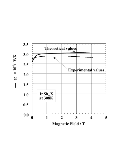
Figure 1: Thermoelectric power versus magnetic field of InSb_X at 308K

Figure 2: Nernst Coefficient multiplied by magnetic field $NB$ versus magnetic field of InSb_X at 308K

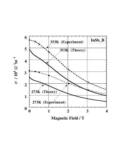
Figure 3: Electrical conductivity versus magnetic field of InSb_B at 273K and 353K

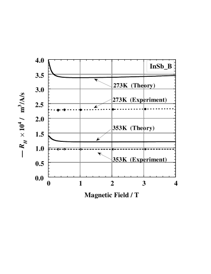
Figure 4: Hall coefficient versus magnetic field of InSb_B at 273K and 353K

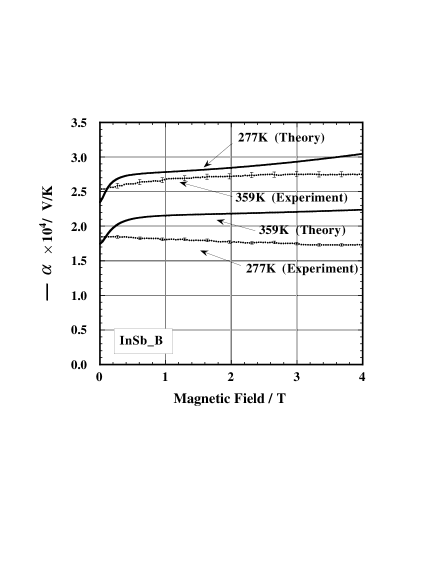
Figure 5: Thermoelectric power versus magnetic field of InSb_B at 273K and 353K

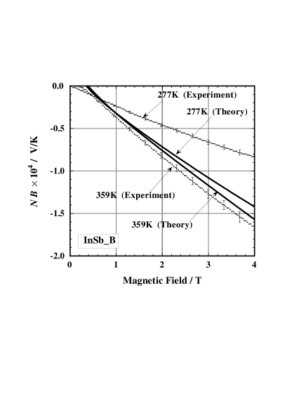
Figure 6: Nernst coefficient multiplied by magnetic field $NB,$ versus magnetic field of InSb_B at 273K and 353K

4 Discussion and conclusions

From comparison the experimental and the theoretical values, we conclude that the two-band model is enough good model to estimate the transport coefficient. We need to measure thermal conductivity to estimate the thermomagnetic (i.e. Nernst ) figure-of-merit $Z_{N}=\sigma(NB)^{2}/\kappa.$ The thermal conductivity has phonon scattering mechanism. We, therefore, improve the physical model to include the phonon scattering phenomena. This is a future problem.

Acknowledgments
The authors are grateful to Dr. Tatsumi in Sumitomo Electric Industries. We appreciate Prof. Iiyoshi and Prof. Motojima in the National Institute for Fusion Science for his helpful comments.

References

• [1] S. Yamaguchi, A. Iiyoshi, O. Motojima, M. Okamoto, S. Sudo, M. Ohnishi, M. Onozuka and C. Uesono, ”Direct Energy Conversion of Radiation Energy in Fusion Energy , Proc. of 7th Int. Conf. Merging Nucl. Energy Systems (ICENES), (1994) 502.
• [2] S. Yamaguchi, K. Ikeda, H. Nakamura and K. Kuroda, A Nuclear Fusion Study of Thermoelectric Conversion in Magnetic field , 4th Int. Sympo. on Fusion Nuclear Tech., ND-P25, Tokyo, Japan, April (1997).
• [3] T. C. Harman and J. M. Honig, Thermoelectric and Thermomagnetic Effects and Applications, McGraw-Hill, (1967), Chap. 7, p. 311.
• [4] K. Ikeda, H. Nakamura, S. Yamaguchi and K. Kuroda, Measurement of Transport properties of Thermoelectric Materials in the Magnetic Field , J. Adv. Sci., 8 (1996) 147, (in Japanese).
• [5] H. Nakamura, K. Ikeda, S. Yamaguchi and K. Kuroda, Transport Coefficients of Thermoelectric Semiconductor InSb , J. Adv. Sci., 8 (1996) 153, (in Japanese).
• [6] K. Ikeda, H. Nakamura, S. Yamaguchi and I. Yonenaga, Transport Coefficients of InSb, Si and Ge in magnetic fields , 17th Int. Conference on Thermoelectrics, Nagoya, Japan, May(1998) TF-P20 .
• [7] E. H. Putly, The Hall Effect and Related Phenomena, London, Butterworth &Co. Ltd., (1960), Chap. 3.
• [8] H. Nakamura, K. Ikeda and S. Yamaguchi, Transport Coefficients of InSb in a Strong Magnetic Field , Proc. of 16th Int. Conference on Thermoelectrics, Dresden, Germany, Augusut (1997) p. 142.