Elements for a Theory of Financial Risks

Abstract

Estimating and controlling large risks has become one of the main concern of financial institutions. This requires the development of adequate statistical models and theoretical tools (which go beyond the traditionnal theories based on Gaussian statistics), and their practical implementation. Here we describe three interrelated aspects of this program: we first give a brief survey of the peculiar statistical properties of the empirical price fluctuations. We then review how an option pricing theory consistent with these statistical features can be constructed, and compared with real market prices for options. We finally argue that a true ‘microscopic’ theory of price fluctuations (rather than a statistical model) would be most valuable for risk assessment. A simple Langevin-like equation is proposed, as a possible step in this direction.

1 Introduction

The efficiency of the theoretical tools devised to address the problems of risk control, portfolio selection and derivative pricing strongly depends on the adequacy of the stochastic model chosen to describe the market fluctuations. Historically, the idea that price changes could be modelled as a Brownian motion dates back to Bachelier [1]. This hypothesis, or some of its variants (such as the Geometrical Brownian motion, where the log of the price is a Brownian motion) is at the root of most of the modern results of mathematical finance, with Markowitz portfolio analysis, the Capital Asset Pricing Model (capm) [2] and the Black-Scholes formula [3] standing out as paradigms. The reason for success is mainly due to the impressive mathematical and probabilistic apparatus available to deal with Brownian motion problems, in particular Ito’s stochastic calculus.

An important justification of the Brownian motion description lies in the Central Limit Theorem (clt), stating that the sum of $N$ identically distributed, weakly dependent random changes is, for large $N$, a Gaussian variable. In physics or in finance, the number of elementary changes observed during a time interval $t$ is given by $N={t\over\tau^{*}}$ where $\tau^{*}$ is an elementary correlation time, below which changes of velocity (for the case of a Brownian particle) or changes of ‘trend’ (in the case of the stock prices) cannot occur. The use of the clt to substantiate the use of Gaussian statistics in any caserequires that $t\gg\tau^{*}$. In financial markets, $\tau^{*}$ turns out to be of the order of several minutes, which is not that small compared to the relevant time scales (days), in particular when one has to worry about the tails of the distribution (corresponding to large shocks) which sometimes disappear only very slowly.

The fact that the tails of the distribution of returns are much ‘fatter’ than predicted by the gaussian is well known, in particular since the seminal work of Mandelbrot [4], where the idea that price changes are still independent, but distributed according to a Lévy stable law was first proposed. This model however fails in two respects. First, the tails of the distribution of returns is now much overestimated; in particular, the variance appears to be well defined in most financial markets, while it is infinite for Lévy distributions. Second, and perhaps more importantly in view of its application to option markets, the amplitude of the fluctuations (measured, say, as the local variance) appears to be itself a randomly fluctuating variable with rather long range correlations.

The aim of this paper is to provide a short survey of the most prominent statistical properties of the fluctuations of rather liquid markets, which are characterized by what one could call ‘moderate’ fluctuations (for a review, see e.g. [5]). Less liquid markets sometimes behave rather differently and more ‘extreme’ fluctuations can be observed. We shall then present a theory for option pricing and hedging in the general case where the underlying stock fluctuations are not gaussian. In this case, perfect hedging is in general impossible, but optimal strategies can be found (analytically or numerically) and the associated residual risk can be estimated. We show that the volatility ‘smile’ observed on option markets can be understood using a cumulant expansion, and discuss the idea of an implied ‘kurtosis’, which is (on liquid markets) very close to the actual (maturity dependent) kurtosis of the historical data. Finally, we briefly discuss a simple ‘Langevin’ approach to market fluctuations, which aims at describing, in a coarse-grained way, the feedback effects between the agents behaviour and the price fluctuations. Interestingly, a natural distinction appears between a normal regime, where price fluctuations are moderate, from a ‘crash’ regime, where panic effects are self-reinforcing and leads to a price collapse.

2 A Short Survey of Empirical Data

2.1 Linear correlations

We shall denote in the following the value of the stock (or any other asset) at time $t$ as $x(t)$, and the variation of the stock on a given time interval $\tau$ as $\delta_{\tau}x(t)=x(t+\tau)-x(t)$. The time delay $\tau$ can be as small as a few seconds in actively traded markets. However, on these short time scales, the fluctuations cannot be considered to be independent. For example, the second order correlation function defined as :

$$C(\Delta t)=\frac{\langle\delta_{\tau}x(t+\Delta t)\delta_{\tau}x(t)\rangle}{\langle\delta_{\tau}x(t)^{2}\rangle}$$ (1)

is significantly non-zero up to $\Delta t=15$ minutes, as shown in Fig. 1.

Figure 1: Correlation function $C(\Delta t)$ of the one minute price increments of the S&P 500, for the period 1983-1996, which decays to zero on the scale of $\tau^{*}\simeq 15$ minutes. Note that $\tau^{*}$ has drifted to smaller values with time.

Therefore, it is certainly inadequate to think of the price process as a ‘martingale’ for small time increments. This however does not necessarily mean that there are arbitrage opportunities: one can easily see that even very small transaction costs prevent the use of these short time correlations, which would imply a very high (and thus very costly) trading frequency [6]. For time delays $\Delta t$ longer than a certain $\tau^{*}$, say one hour, the autocorrelation of price increments is very nearly zero; correspondingly, the variance of price increments grow linearly with $\Delta t$ for $\Delta t>\tau^{*}$.

2.2 Distribution of elementary increments

The simplest idea is thus that the increments $\delta(t)$ are independent identically distributed (iid) random variables. In this case, the knowledge of the distribution density $P^{*}$ of $\delta$ would suffice to reconstruct the distribution of increments on any time delay $\Delta t$ larger than $\tau^{*}$, through a simple convolution. The shape of $P^{*}$ is strongly non gaussian: an estimate of its kurtosis $\kappa_{\tau^{*}}$ on a historical basis leads to numbers on the order of $20$ (again on liquid markets). As shown in Fig. 2 on the example of the British Pound/U.S. $ time series, the tails of $P^{*}$ decay as an exponential:

$$P(\delta)\propto\exp\left(-\lambda_{\pm}|\delta|\right)\qquad\delta\to\pm\infty$$ (2)

(although several authors have reported a somewhat slower decay, as a power law $|\delta|^{-1-\nu}$ with a rather large exponent $\nu\simeq 3$–$4$ [7], or possibly a ‘stretched exponential’ [8]). Such slowly decaying tails survive upon convolution, and are thus particularly relevant for extreme risks forecasts [10].

Figure 2: Distribution of the British Pound/US $ negative increments for $\tau^{*}=30$ mimutes, in the period 1991-1995. The ‘near-tail’ of the distribution can be fitted by a power-law, which clearly overestimates the ‘far-tail’. The latter is well represented by an exponential fall-off, Eq. (2): note the linear-log scale

A reasonable fit of $P^{*}$ on most markets can be achieved using a symmetrical ‘truncated’ Lévy distribution[9, 6], defined in Fourier space as:

$$\log P^{*}(z)=\frac{A}{\cos\pi\mu/2}\left[{\lambda^{\mu}}-(\lambda^{2}+z^{2})^{\mu/2}f(z)\right];\quad f(z)=\cos\left(\mu\arctan\frac{|z|}{\lambda}\right)$$ (3)

where $A$ the scale factor, $\mu$ is the ‘tail exponent’, which is found to be close to $1.5$ for all markets, and $\lambda$ describes the exponential fall of the far-tails. Note that when $\mu=2$, one recovers the gaussian distribution, while for $\lambda\to 0$, one finds the stable Lévy distributions proposed by Mandelbrot [4], with tails which decay as $|\delta|^{-1-\mu}$.

2.3 Anomalous decay of the kurtosis and volatility persistence

The $N^{th}$ autoconvolution of $P^{*}$, where $N=\Delta t/\tau^{*}$ is simply obtained by scaling the parameter $A$ to $NA$. With no further ajustable parameters, this leads to a fair representation of the historical distribution of $\delta_{\Delta t}x$ [6, 11]. However, some systematic differences (in particular in the tails of the distribution) show up, which reveal the inadequacy of such a simple iid hypothesis. For example, it is easy to show that under such an hypothesis, the kurtosis of the increments on scale $\Delta t=N\tau^{*}$ should be a factor $N$ smaller than the kurtosis on scale $\tau^{*}$. Empirically, however, one finds a much slower decay, as $\kappa_{N}=\kappa_{1}/N^{\lambda}$, with $\lambda$ in the range $0.3-0.6$ (see Fig. 3). This can be related to another observation, which was made many times in the literature [5, 12]: higher order correlation functions of the price increments, such as:

$$C_{2}(m)=\frac{\langle\delta^{2}(t+m\tau^{*})\delta^{2}(t)\rangle}{\langle\delta^{2}(t)\rangle^{2}}-1$$ (4)

decay only very slowly with time. A simple fit of this decay is again of the power law type [5, 13, 14]:

$$C_{2}(m)\simeq\frac{C_{0}}{m^{\lambda^{\prime}}}$$ (5)

with a exponent $\lambda^{\prime}$ in the same range as $\lambda$. A simple way to rationalize these findings is to assume that while the sign of the price increment is completely decorrelated as soon as $\Delta t>\tau^{*}$, the amplitude of the increment (which is a measure of the market activity) is correlated in time. Bursts of market activity, related to external news or crisis, can easily persist for several days, sometimes months – this explains why $C_{2}(m)$ decays rather slowly. We shall thus assume that the increment $\delta$ can be written as:

$$\delta(t_{i})=\gamma(t_{i})\times\epsilon(t_{i})\qquad t_{i}=i\tau^{*}$$ (6)

where the scale $\gamma>0$ measures the amplitude of the increment, which can be thought of as the local volatility of the market. The random variable $\epsilon$ is short range correlated (over time $\tau^{*}$) of mean zero and variance unity (and independent from $\gamma$). Note that $\epsilon$ is not necessarily Gaussian, as assumed in arch-like models [12]. It is then rather easy to show that the kurtosis of the increments on scale $\Delta t=N\tau^{*}$ can be expressed as [15, 6]:

$$\kappa_{N}=\frac{1}{N}\left[\kappa_{0}+(3+\kappa_{0})C_{2}(0)+6\sum_{m=1}^{N}(1-\frac{m}{N})C_{2}(m)\right]$$ (7)

where $\kappa_{0}$ is the kurtosis of the random variable $\epsilon$. Note that even if $\kappa_{0}=0$, the kurtosis of $P^{*}$ is non zero due to the randomly fluctuating scale parameter $\gamma$. If one furthermore assumes that $C_{2}$ decays as a power-law (Eq. 5), then from Eq. (7), $\kappa_{N}$ decays for large $N$ as $N^{-\lambda}$ with $\lambda=\lambda^{\prime}$.

2.4 Apparent (multi)-scaling behaviour

Hence, the fact that the scale $\gamma$ of the random increments has long range temporal correlations induces an anomalously slow convergence of the sum $x({N\tau^{*}})-x(0)=\sum_{i=1}^{N}\delta(t_{i})$ towards the gaussian distribution. One should note that this can induce apparent scaling behaviour on restricted time intervals. For example, a numerical simulation of the random scale model (6) with a slowly decaying $C_{2}(m)$ can be analyzed in scaling terms [16], i.e. fitting the moments of $x({N\tau^{*}})-x(0)$ as power laws:

$$\langle|x({N\tau^{*}})-x(0)|^{q}\rangle\propto N^{\zeta_{q}}$$ (8)

This actually works quite well, and leads to a family of exponents $\zeta_{q}$ which deviates from the theoretical straight line $\zeta_{q}=q/2$ which holds in the limit $N\to\infty$, provided all the moments of $\gamma$ exist. For $q=2$, the relation $\zeta_{2}=1$ holds because the linear correlation function $C(\Delta t)$ is zero for $\Delta t>\tau^{*}$. For $q=4$ one finds, using the definition of the kurtosis:

$$\langle[x({N\tau^{*}})-x(0)]^{4}\rangle=(3+\kappa_{N})\langle[x({N\tau^{*}})-x(0)]^{2}\rangle^{2}\propto 3N^{2}+\kappa_{1}N^{2-\lambda}$$ (9)

which is thus the sum of two power laws. This can be however fitted with a unique ‘effective’ exponent $\zeta_{4}$, which can be substantially below the asymptotic value $\zeta_{4}^{\infty}=2$ since $N^{-\lambda}$ is not very small in practice. This argument holds true for higher moments for which $\zeta_{q}<q/2$; the difference between $\zeta_{q}$ and $q/2$ actually grows with $q$ (for a fixed value of $N$). We believe that this might be the reason for the ‘multifractal’ scaling recently reported in the literature [17, 18].

2.5 Time reversal symmetry

The last empirical fact which we would like to comment on is the question of time reversal symmetry. Is it possible to detect the direction of time in a financial time series ? The answer to this question would be no for a simple Brownian motion, for example, but also for a much wider class of processes, such as the multifractal time construction proposed in [18]. Correlation functions sensitive to the arrow of time have been proposed by Pomeau [19]. One example is:

$$C_{T}(\Delta t)=\langle x(t)\left[x(t+\Delta t)-x(t+2\Delta t)\right]x(t+3\Delta t)\rangle$$ (10)

which is non zero if the time triplets $t,t+\Delta t,t+3\Delta t$ and $t,t+2\Delta t,t+3\Delta t$ cannot be distinguished statistically. For the price series itself, the above correlation function is zero within error bars. But when one studies the ‘volatility’ process $\gamma$, then this skew correlation function is distinctively non zero, and reaches a maximum (in the case of the S&P 500) for $\Delta t\simeq$ 1 month. This shows that the volatility time series is not invariant under time reversal. A similar conclusion is also reported in [20, 14], where the authors observe that a high ‘coarse-grained’ volatility in the past increases in a causal way today’s ‘fine-grained’ volatility. This is not unreasonable, as one feels intuitively that an anomalously large change of the close to close price over – say – the previous week triggers more intraday activity the following week. In any case, we feel that this absence of time reversal symmetry is an important (albeit less frequently discussed) stylized fact of financial time series.

3 Implications for Option Pricing

3.1 General framework

We now turn to the problem of option pricing and hedging when the statistics for price increments have the non-Gaussian properties discussed above. The distinctive feature of the continuous time random walk model usually considered in the theory of option pricing is the possibility of perfect hedging [21], that is, a complete elimination of the risk associated to option trading [3]. This property however no longer holds for more realistic models [22].

Let us write down the global wealth balance $\Delta W|_{0}^{T}$ associated with the writing of a ‘call’ option of maturity $T$ and exercice price $x_{s}$ [6]:

$$\Delta W|_{0}^{T} = {\cal C}(x_{0},x_{s},T)\exp(rT)-\max(x(T)-x_{s},0)$$ (11)

$$+ \sum_{i}\ \phi(x,t_{i})\exp(r(T-t_{i}))[\delta_{i}-rx(t_{i})\tau],$$ (12)

where ${\cal C}(x_{0},x_{s},T)$ is the price of the call, $x_{0}=x(t=0)$ and $\phi(x,t)$ the trading strategy, i.e. the number of stocks per option in the portfolio of the option writer. Finally, $r$ the (constant) interest rate. The second term defines the option contract: the profit of the buyer of the option is equal to $x_{s}-x(T)$ if $x(T)>x_{s}$ (i.e. if the option is exercised) and zero otherwise: the option is an insurance contract which guarantees to its owner a maximum price for acquiring a certain stock at time $T$. Conversely, a ‘put’ option would guarantee a certain minimum price for the stock held by the owner of the option.

A natural procedure to fix the price of the option ${\cal C}(x_{0},x_{s},T)$ and the optimal strategy $\phi^{*}(x,t)$ was proposed independently in [23, 22] and further discussed in [6, 24, 25]. It consists in imposing a fair game condition, i.e.:

$$\langle\Delta W|_{0}^{T}[\phi]\rangle=0$$ (13)

and a risk minimisation condition:

$$\left.\frac{\delta\langle\Delta W|_{0}^{T}[\phi]^{2}\rangle}{\delta\phi(x,t)}\right|_{\phi^{*}}=0$$ (14)

Here, we assume that the variance of the wealth variation is a relevant measure of the risk. However, other measures are possible, in particular the ‘Value-at-Risk’, which is directly related to the weight contained in the negative tails of the distribution of $\Delta W|_{0}^{T}$.

The notation $\langle...\rangle$ in Eqs. (13,14) means that one averages over the probability of the different trajectories. The explicit solution of Eqs. (13,14) for a general uncorrelated process (i.e. $\langle\delta_{i}\delta_{j}\rangle=0$ for $i\neq j$) is relatively easy to write if the average bias $\langle\delta\rangle$ and the interest rate $r$ are negligible, which is the case for short maturities $T$. In this case, one finds [22]:

$${\cal C}(x_{0},x_{s},T)=\int_{x_{s}}^{\infty}dx^{\prime}\ (x^{\prime}-x_{s})P(x^{\prime},T|x_{0},0)$$ (15)

$$\phi^{*}(x,t)=\int_{x_{s}}^{\infty}dx^{\prime}\langle\delta\rangle_{(x,t)\longrightarrow(x^{\prime},T)}{(x^{\prime}-x_{s})\over{\sigma^{2}}(x,t)}P(x^{\prime},T|x,t)$$ (16)

where $\sigma^{2}(x,t)=\langle\delta^{2}\rangle|_{x,t}$ is the ‘local volatility’ – which may depend on $x,t$ – and $\langle\delta\rangle_{(x,t)\longrightarrow(x^{\prime},T)}$ is the mean instantaneous increment conditioned to the initial condition $(x,t)$ and a final condition $(x^{\prime},T)$. The minimal residual risk, defined as ${\cal R}^{*}=\langle\Delta W|_{0}^{T}[\phi^{*}]^{2}\rangle$ is in general strictly positive (and in practice rather large), except for Gaussian fluctuations in the continuous limit, where the residual risk is strictly zero! In this limit, the above equations (13,14) actually exactly lead to the celebrated Black-Scholes option pricing formula. In particular, one can check that $\phi^{*}$ is related to ${\cal C}$ through: $\phi^{*}=\partial{\cal C}(x_{0},x_{s},T)/{\partial x_{0}}$.

3.2 Cumulant expansion and volatility smile

In the case where the market fluctuations are moderately non-Gaussian, one might expect that a cumulant expansion around the Black-Scholes formula leads to interesting results. This cumulant expansion has been worked out in general in [6]. If one only retains the leading order correction which is (for symmetric fluctuations) proportional to the kurtosis, one finds that the price of options ${\cal C}(x_{0},x_{s},T)$ can be written as a Black-Scholes formula, but with a modified value of the volatility $\sigma$, which becomes price and maturity dependent [15]:

$$\sigma_{imp.}(x_{s},T)=\sigma\left[1+\frac{\kappa_{T}}{24}\left(\frac{(x_{s}-x_{0})^{2}}{\sigma^{2}T}-1\right)\right]$$ (17)

The volatility $\sigma_{imp.}$ is called the implied volatility by the market operators, who use the standard Black-Scholes formula to price options, but with a value of the volatility which they estimate intuitively, and which turns out to depend on the exercice price in a roughly parabolic manner, as indeed suggested by Eq. (17).

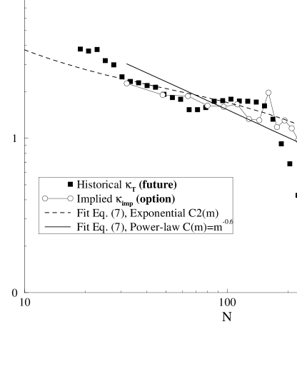
Figure 3: Plot (in log-log coordinates) of the average implied kurtosis $\kappa_{imp}$ (determined by fitting the implied volatility for a fixed maturity by a parabola) and of the empirical kurtosis $\kappa_{N}$ (determined directly from the historical movements of the bund contract), as a function of the reduced time scale $N=T/\tau$, $\tau=30$ minutes. All transactions of options on the bund future from 1993 to 1995 were analyzed along with 5 minute tick data of the bund future for the same period. We show for comparison a fit with $\kappa_{N}\simeq N^{-0.6}$ (dark line). A fit with an exponentially decaying $C_{2}(m)$ is however also acceptable (dotted line).

This is the so-called ‘volatility smile’. Eq. (17) furthermore shows that the curvature of the smile is directly related to the kurtosis of the underlying statistical process on the scale of the maturity $T=N\tau^{*}$. We have tested this prediction by directly comparing the ‘implied kurtosis’, obtained by extracting from real option prices (on the bund market) the volatility $\sigma$ (which turns out to be highly correlated with a short time filter of the historical volatility), and the curvature of the implied volatility smile, to the historical value of the kurtosis $\kappa_{N}$ discussed above. The result is plotted in Fig. 3, with no further ajustable parameter. The remarkable agreement between the implied and historical kurtosis, and the fact that they evolve similarly with maturity, shows that the market as a whole is able to correct (by trial and errors) the inadequacies of the Black-Scholes formula, and to encode in a satisfactory way both the fact that the distribution has a positive kurtosis, and that this kurtosis decays in an anomalous fashion due to volatility persistence effects. However, the real risks associated with option trading are, at present, not satisfactorily estimated. In particular, most risk control softwares dealing with option books are based on a Gaussian description of the fluctuations.

4 A Langevin Approach to Price Fluctuations: Feedback Effects

In the author’s opinion, there is as yet no convincing ‘microscopic’ model which explains the distinctive statistical features of price fluctuations which were summarized in section 2, although many proposals have been put forward [26, 27]. In the spirit of statistical physics, it might be possible to describe market dynamics at a level of description which is intermediate between the macroeconomic level which is that of the market equilibrium models [26] and the individual agent level which is that of the market microstructure theory. Our basic idea is that although the modelling of each individual participants (‘agents’) is impossible in quantitative terms, the collective behavior of the market and its impact on the price in particular can be represented in statistical terms by a few number of terms in a (stochastic) dynamical equation. Our approach is in the spirit of many phenomenological, ‘Landau-like’ approaches to physical phenomena [28]. We have thus proposed a description of the dynamics of speculative markets with a simple Langevin equation [29]. This equation encapsulates what we believe to be some essential ingredients; in particular, the feedback of the price fluctuations on the behaviour of the market participants. The construction of a convincing model for large fluctuations is important for risk control, since empirical data may be unreliable in the extreme tails of the distributions.

4.1 A Phenomenological Langevin Equation

At any given instant of time, there is a certain number of ‘buyers’ which we call $\phi_{+}(t)$ (the demand) and ‘sellers’, $\phi_{-}(t)$ (the supply). The first dynamical equation describes the effect of an offset between supply and demand, which tends to push the price up (if $\phi_{+}>\phi_{-}$) or down in the other case. In general, one can write:

$$\frac{dx}{dt}={\cal F}(\Delta\phi)\qquad\Delta\phi:=\phi_{+}-\phi_{-}$$ (18)

where ${\cal F}$ is an increasing function, such that ${\cal F}(0)=0$. In the following, we will frequently assume that ${\cal F}$ is linear (or else that $\Delta\phi$ is small enough to be satisfied with the first term in the Taylor expansion of ${\cal F}$), and write

$$\frac{dx}{dt}=\frac{\Delta\phi}{\lambda}$$ (19)

where $\lambda$ is a measure of market depth i.e. the excess demand required to move the price by one unit. When $\lambda$ is high, the market can ‘absorb’ supply/demand offsets by very small price changes. Now, we try to construct a dynamical equation for the supply and demand separately. Consider for example the number of buyers $\phi_{+}$. Between $t$ and $t+dt$, a certain fraction of those get their deal and disappear (at least temporarily). This deal is usually ensured by market makers, which act as intermediaries between buyers and sellers. The role of market markers is to absorb the demand (and supply) even if these do not match perfectly. The effect of market makers (mm) can thus be modelled as:

$$\left.\frac{d\phi_{\pm}}{dt}\right|_{{\sc mm}}=-\Gamma_{\pm}\phi_{\pm}$$ (20)

where $\Gamma_{\pm}$ are rates (inverse time scales). We furthermore assume that market makers act symmetrically, i.e, that $\Gamma_{+}=\Gamma_{-}=\gamma$. On liquid markets, the time scale $1/\gamma$ before which a deal is reached is short; typically a few minutes (see also below for another interpretation of $1/\gamma$).

There are several other effects which must be modeled to account for the time evolution of supply and demand. One is the spontaneous (sp) appearance of new buyers (or sellers), under the influence of new information, individual need for cash, or particular investment strategies. This can be modelled as a white noise term (not necessarily Gaussian):

$$\left.\frac{d\phi_{\pm}}{dt}\right|_{{\sc sp}}=m_{\pm}(t)+\eta_{\pm}(t)$$ (21)

where $\eta_{\pm}$ have zero mean, and a short correlation time $\tau_{c}$. $m_{\pm}$ is the average increase of demand (or supply), which might also depends on time through the time dependent anticipated return $R(t)$ and the anticipated risk $\Sigma(t)$. It is quite clear that both these quantities are constantly reestimated by the market participants, with a strong influence of the recent past. For example, ‘trend followers’ extrapolate a local trend into the future. On the other hand, ‘fundamental analysts’ estimate what they believe to be the ‘true’ price of the stock; if the observed price is above this ‘true’ price, the anticipated trend is reduced, and vice-versa. In mathematical terms, these effects can be represented as:

$$R(t)=R_{0}+\alpha\int_{-\infty}^{t}dt^{\prime}K_{R}(t-t^{\prime})\frac{dx}{dt^{\prime}}-\kappa(x-x_{0})$$ (22)

where $K_{R}$ is a certain kernel (of integral one) defining how the past average trend is measured by the agents, and $\kappa$ is a mean-reversion force, towards the average (over the fundamental analysts) ‘true price’ $x_{0}$ .

Similarly, the anticipated risk has a short time scale contribution. It is well known that an increase of volatility is badly felt by the agents, who immediately increase their estimate of risk. Hence, we write:

$$\Sigma(t)=\Sigma_{0}+\beta\int_{-\infty}^{t}dt^{\prime}K_{\Sigma}(t-t^{\prime})\left[\frac{dx}{dt^{\prime}}\right]^{2}$$ (23)

Correspondingly, expanding $m_{\pm}(R,\Sigma)$ to lowest order, one has:

$$m_{\pm}=m_{0\pm}+\alpha_{\pm}\int_{-\infty}^{t}dt^{\prime}K_{R}(t-t^{\prime})\frac{dx}{dt^{\prime}}+\beta_{\pm}\int_{-\infty}^{t}dt^{\prime}K_{\Sigma}(t-t^{\prime})\left[\frac{dx}{dt^{\prime}}\right]^{2}-\kappa_{\pm}(x-x_{0})$$ (24)

where the signs of the different coefficients are set by the observation that $m_{+}$ is an increasing function of return $R$ and a decreasing function of risk $\Sigma$, and vice versa for $m_{-}$. Eq. (24) contains the leading order terms which arise if one assumes that the agents try to reach a tradeoff between risk and return: the demand for an asset decreases if is recent evolution shows high volatility and increases if it shows an upward trend. This is the case for example if the investors follow a mean-variance optimisation scheme with adaptive estimates of risk and return [2], or the Black-Scholes option hedging strategy [3]. Actually, the 1987 crash is often attributed (at least in part) to the automatic use of the Black-Scholes hedging strategy, which automatically generates sell orders when the value of the stock goes down.

We are now in position to write an equation for the supply/demand offset $\Delta\phi$ by summing all these different contributions:

$$\frac{d\Delta\phi}{dt} = -\gamma\Delta\phi+m_{0}+a\int_{-\infty}^{t}dt^{\prime}K_{R}(t-t^{\prime})\frac{dx}{dt^{\prime}}$$ (25)

$$- b\int_{-\infty}^{t}dt^{\prime}K_{\Sigma}(t-t^{\prime})\left[\frac{dx}{dt^{\prime}}\right]^{2}-k(x-x_{0})+\eta(t)$$

with $a,b,k>0$. Note in particular that $b>0$ reflects the fact that agents are risk averse, and that an increase of the local volatility always leads to negative contribution to $\Delta\phi$. This feature will be crucial in the following. For definiteness, we will consider $\eta$ to be gaussian and normalize it as:

$$\langle\eta(t)\eta(t^{\prime})\rangle=2\lambda^{2}D\delta(t-t^{\prime})$$ (26)

where $D$ measure the susceptibility of the market to the random external shocks, typically the arrival of information. As discussed in section 2, $D$ should also depend on the recent history, reflecting the fact that an increase in volatility induces a stronger reactivity of the market to external news. In the same spirit as above, one could thus write:

$$D=D_{0}+D_{1}\int_{-\infty}^{t}dt^{\prime}K_{D}(t-t^{\prime})\left[\frac{dx}{dt^{\prime}}\right]^{2}$$ (27)

For simplicity, we will neglect the influence of $D_{1}$ in the following. But such a term might be responsible for the time reversal symmetry breaking effect reported in section 2, as well as for the fact that volatility appears to be time dependent.

4.2 Simple consequences. Liquid vs. Illiquid markets

Let us consider the linear case ‘risk neutral’ case where $b=0$. We will assume for simplicity that $K_{R}(t)=\Gamma\exp-(\Gamma t)$, and first consider the local limit where $\Gamma$ is much larger that $\gamma$ (short memory time). In this case, the equation for $x$ becomes that of an harmonic oscillator:

$$\frac{d^{2}x}{dt^{2}}+\left(\gamma-\frac{a}{\lambda}\right)\frac{dx}{dt}+\frac{k}{\lambda}(x-\tilde{x}_{0})=\frac{1}{\lambda}\eta(t)$$ (28)

where $m_{0}$ has been absorbed into a redefinition of $\tilde{x}_{0}:=x_{0}+m_{0}/k$. For liquid markets, where $\lambda$ and $\gamma$ are large enough, the ‘friction’ term $\tilde{\gamma}:=\gamma-a/\lambda$ is positive. In this case the market is stable, and the price oscillates around an equilibrium value $\tilde{x}_{0}$, which is higher than the average fundamental price if the spontaneous demand is larger than the spontaneous supply (i.e. $m_{0}$ is positive), as expected when the overall economy grows. The situation is rather different for illiquid markets, or when trend following effects are large, since $\tilde{\gamma}$ can be negative. In this case, the market is unstable, with an exponential rise or decay of the stock value, corresponding to a speculative bubble. However, in this case, $dx/dt$ grows with time and it soon becomes untenable to neglect the higher order terms, in particular the risk aversion term proportional to $b$, which is responsible for a sudden collapse [29].

4.3 Risk aversion induced crashes

In the case of liquid markets on short time scales, it is reasonnable to set $k=0$ [29]. Setting $u=dx/dt$ and still focusing on the limit where the memory time $\Gamma^{-1}$ is very small, one finds the following non linear Langevin equation:

$$\frac{du}{dt}=\frac{m_{0}}{\lambda}-\tilde{\gamma}u-\frac{b}{\lambda}u^{2}+\frac{1}{\lambda}\eta(t)\equiv-\frac{\partial V}{\partial u}+\frac{1}{\lambda}\eta(t)$$ (29)

This equation represents the evolution of the position $u$ of a viscous fictitious particle in a ‘potential’ $V(u)$. In order to keep the mathematical form simple, we set the average trend $m_{0}/\lambda$ to zero (no net average offset between spontaneous demand and spontaneous supply); this does not qualitatively change the following picture, unless $m_{0}$ is negative and large. The potential $V(u)$ can then be written as:

$$V(u)=\frac{\tilde{\gamma}}{2}u^{2}+\frac{b}{3\lambda}u^{3}$$ (30)

which has a local minimum for $u=0$, and a local maximum for $u^{*}=-\lambda\tilde{\gamma}/b$, beyond which the potential plumets to $-\infty$. The ‘barrier height’ $V^{*}$ separating the stable region around $u=0$ from the unstable region is given by:

$$V^{*}=V(u^{*})-V(0)=\frac{\tilde{\gamma}u^{*2}}{6}$$ (31)

The nature of the motion of $u$ in such a potential is the following: starting at $u=0$, the particle has a random harmonic-like motion in the vicinity of $u=0$ until an ‘activated’ event (i.e. driven by the noise term) brings the particle near $u^{*}$. Once this barrier is crossed, the fictitious particle reaches $-\infty$ in finite time. In financial terms, the regime where $u$ oscillates around $u=0$ and where $b$ can be neglected, is the ‘normal’ random walk regime discussed in the previous paragraph. (Note that the random walk is biased when $m_{0}\neq 0$). This normal regime can however be interrupted by ‘crashes’, where the time derivative of the price becomes very large and negative, due to the risk aversion term $b$ which enhances the drop in the price. The point is that these two regimes can be clearly separated since the average time $t^{*}$ needed for such crashes to occur can be exponentially long, since it is given by the classical Arrhenius-Kramers formula [30, 31]:

$$t^{*}=2\pi\tau_{1}\exp\left(\frac{V^{*}}{D}\right)=\frac{2\pi}{\gamma}\exp\left(\frac{u^{*2}\tau_{1}}{3\sigma^{2}}\right)$$ (32)

where $D$ is the variance of the noise $\eta$ and $\tau_{1}=1/\tilde{\gamma}$. Taking $t^{*}=10$ years, $\sigma=1\%$ per day, and $\tau_{1}=10$ minutes, one finds that the characteristic value $u^{*}$ beyond which the market ‘panics’ and where a crash situation appears is of the order of $-1\%$ in ten minutes, which not unreasonnable. Note that in this line of thought, a crash occurs because of an improbable succession of unfavorable events, and not due to a single large event in particular. Furthermore, there are no ‘precursors’ - characteristic patterns observed before the crash: before $u$ has reached $u^{*}$, it is impossible to decide whether it will do so or whether it will quietly come back in the ‘normal’ region $u\simeq 0$. Note finally that an increase in the liquidity factor $\gamma$ reduces the probability of crashes. This is related to the stabilizing role of market makers, which appears very clearly.

The above calculations can be extended to the case where the ‘integration time’ of the market (appearing in the kernels $K_{R}$ and $K_{\Sigma}$) is not very short, with very similar conclusions [29].

5 Conclusion

Research on financial markets can focus on rather different aspects. We have discussed here three interrelated themes: the statistical nature of the market fluctuations, its use for option pricing and the need for a microsocopic ‘explicative’ model which accounts for empirical observations. We have emphasized the fact that a good model of these fluctuations was crucial to estimate and control large risks. This requires in particular an adapted theory for option pricing, which goes beyond the traditionnal Black-Scholes dogma. We have shown that subtle statistical effects, such as the persistence of volatility fluctuations, is rather well reflected in option prices. This shows that the market as a whole behaves as an adaptive system, able to correct (through trial and errors) the theoretical inadequacies of the Black-Scholes formula.

The theoretical understanding of the tails of the distributions is furthermore of fundamental importance, because by definition the empirical observation of rare events leads does not allow one to determine the extreme tails of the distribution with great accuracy. In this respect, an interesting aspect of the Langevin equation discussed above is that crashes events appear as fundamentally distinct from ‘normal’ events, and their probability of occurence is thus not expected to lie on the extrapolation of the (non Gaussian) distribution constructed from these ‘normal’ events. This is actually what is observed: although the empirical tail of the distribution of the S&P 500’s daily increments is pretty well fitted by an exponential down to probabilities of $10^{-3}$, events which have a probability of $10^{-4}$ (i.e. crashes which occcur once every 40 years) have an amplitude which is much larger than expected [32].

There are many other aspects of financial markets which are worth investigating using the tools and ideas of statistical physics, which we have not discussed here at all: we refer the reader to the recent literature, which can be found on the preprint server “cond-mat”[33]. One of the most exciting subject is the modelling of the interest curve, which might have a lot in common with the dynamics of an elastic string driven by noise [34].

Acknowledgements

This work is the result of many collaborations, which started with D. Sornette and continued in a most fruitful and enjoyable way with Rama Cont and M. Potters. I also want to acknowledge important discussions with J.P. Aguilar, E. Aurell, P. Cizeau and L. Laloux.

References

- [1] L. Bachelier, ‘Theory of Speculation’ (translation of 1900 French edition), 17–78, in The Random Character of Stock Market Prices, P. H. Cootner (ed.), MIT Press, (1964).
- [2] R. C. Merton, Continuous-Time Finance, Blackwell, (1990).
- [3] F. Black, M. Scholes, Journal of Political Economy, 81 (1973) 637.
- [4] B. B. Mandelbrot, Journal of Business 36, 394 (1963); 40, 394 (1967).
- [5] C.W.J. Granger, Z.X. Ding, “Stylized facts on the temporal distributional properties of daily data from speculative markets”; D.M. Guillaume et al., “From the bird’s eye to the microscope”, Finance and Stochastics 1, 2 (1997); R. Cont, M. Potters & J.P. Bouchaud, “Scaling in stock market data: stable laws and beyond” in Scale invariance and beyond, Edts. B. Dubrulle, F. Graner, D. Sornette, EDP Sciences (1997).
- [6] J.P. Bouchaud and M. Potters, Theory of Financial Risk, Aléa-Saclay, Eyrolles (Paris, 1997) (in french).
- [7] see e.g. M.M. Dacorogna, U.A. Muller, O.V. Pictet, C.G. de Vries, “The distribution of extremal exchange rate returns in extremly large data sets”, Preprint of Olsen &A Research Group (1995), available at http://www.olsen.ch, F. Longin, “The asymptotic distribution of extreme stock market returns”, Journal of Business, (1996), P. Gopikrishnan, M. Meyer, L.A. Amaral, H.E. Stanley, cond-mat/9803374.
- [8] J. Laherrère, D. Sornette, cond-mat/9801293.
- [9] R. Mantegna and H.E. Stanley, Phys. Rev. Lett. 28, 2946 (1994); R. Mantegna and H.E. Stanley, Nature 376, 46 (1995).
- [10] A risk-control software designed to deal with ‘fat tails’, based to a large extent on Truncated Lévy Distributions, has been devised by Science & Finance, and is commercialized by atsm under the name Profiler.
- [11] A. Arneodo, J.P. Bouchaud, R. Cont, J.F. Muzy, M. Potters, D. Sornette, cond-mat/9607120, unpublished.
- [12] R. Engle, Econometrica 50 987 (1982); T. Bollerslev, Journal of Econometrics, 31 307 (1986). C. Gourieroux, Modèles ARCH et Applications financières, Economica, Paris (1992).
- [13] P. Cizeau, Y. Liu. M. Meyer, C.K. Peng, H. E. Stanley, cond- mat/9708143.
- [14] A. Arnéodo, J.F. Muzy, D. Sornette, cond-mat/9708012.
- [15] M. Potters, R. Cont, J.P. Bouchaud, Europhys. Lett. 41, 239 (1998)
- [16] J.P. Bouchaud, unpublished (1998).
- [17] see e.g.: S. Ghashghaie, W. Breymann, J. Peinke, P. Talkner and Y. Dodge, Nature 381 767 (1996)
- [18] B. Mandelbrot, Fractals in Finance, Springer (1997).
- [19] Y. Pomeau, J. Physique 43, 859 (1985)
- [20] see the work of M. Dacorogna et al. on ‘harch’ models, work available at http://www.olsen.ch.
- [21] for a remarkable introduction, see: J.C. Hull Futures, Options and Other Derivative Securities, Prentice Hall (1997).
- [22] J. P. Bouchaud & D. Sornette, J. Phys. I France 4, 863 (1994).
- [23] M. Schweizer, The Annals of Probability 22, 1536 (1994). see also M. Schäl, Mathematics of Operations Research 19, 121 (1994).
- [24] E. Aurell, S. Simdyankin, Int. J. of Theo. Appl. Finance, 1, 1 (1998). See also: E. Aurell, K. Życzkowski, ewp-fin/9601001 at http://econwpa.wustl.edu/wpawelcome.html; G. Wolczyńska and O. Hammarlid, to appear in Int. J. of Theo. Appl. Finance (1998).
- [25] A. Matacz, cond-mat/9710197.
- [26] Brock W.A., Hsieh D.A. & LeBaron, B. (1991) Nonlinear dynamics, chaos and instability: statistical theory and economic evidence, Cambridge MA: MIT Press; Grandmont, J.M. “Temporary equilibrium theory” in Arrow, K.J. & Intriligator, M.D. (ed.) (1981) Handbook of mathematical economics, Elsevier; Brock, W.A. & Hommes, C.F. (1997) ”Rational routes to randomness” Econometrica, 65, 1059.
- [27] For recent work in the physics community, see: Bak P., M. Paczuski & M. Shubik (1997) “Price variations in a stock market with many agents”, Physica A. Santa Fe Institute Working Paper; Caldarelli G., Marsili M. & Zhang Y.C. (1997) “A prototype model of stock exchange”, Europhysics Letters, 40 479; R. Cont, J.P. Bouchaud, “Herd behavior and aggregate fluctuations in financial markets”, preprint cond-mat/9712318.
- [28] For a ‘manifesto’ defending such an approach in the physical context, see, e.g. T. Hwa, M. Kardar, Phys. Rev. A 45, 7002 (1992).
- [29] J.P. Bouchaud, R. Cont, “A Langevin approach to stock market fluctuations and crashes”, cond-mat/9801279, submitted to EPJB.
- [30] S. Chandrasekhar, in Noise and Stochastic Processes, N. Wax Editor, Dover, 1954.
- [31] P. Hanggi, P. Talkner, M. Borkovec, Rev. Mod. Phys. 52 (1990) 251.
- [32] A. Johansen, D. Sornette, cond-mat/9712005.
- [33] For an excellent introduction to the relevance of the physical approach in markets, see R. Cont’s PhD Dissertation, ‘From random walks to random markets’, Université d’Orsay (1998), to be published.
- [34] J.P. Bouchaud, N. Sagna, R. Cont, N. ElKaroui, M. Potters, “Phenomenology of the interest rate curve”, cond-mat/9712164, submitted to Applied Mathematical Finance (December 1997). J.P. Bouchaud, N. Sagna, R. Cont, N. ElKaroui, M. Potters, “New Facts on Interest Rates”, to appear in risk Magazine, July 1998.